Retailer’s Procurement Strategy under Endogenous Supply Stability

School of Management, Huazhong University of Science and Technology, No. 1037 Luoyu East Road, Hongshan District, Wuhan 430074, China
*
Author to whom correspondence should be addressed.
Sustainability 2017, 9(12), 2261; https://doi.org/10.3390/su9122261
Submission received: 9 November 2017
/
Revised: 4 December 2017
/
Accepted: 4 December 2017
/
Published: 7 December 2017
(This article belongs to the Special Issue How Retailers Could Contribute to Sustainable Development)
Abstract
:In this paper, a dynamic model is presented to study retailer’s procurement strategy when supply stability is endogenously determined. The optimal supply stability as well as the optimal purchasing strategy are characterized with a quadratic cost function. Based on these models, the following findings are brought about. Firstly, when the difficulty level of building supply stability exceeds a certain threshold, it would be more profitable for the retailer to choose a less reliable supplier. Secondly, given that the suppliers can get positive profit, the retailer would choose the one who has the strongest ability to be reliable. Thirdly, the equilibrium supply to the retailer would always meet the demand on the retailing market. Finally, emergency procurement is shown to be an effective way to reduce the risk of supply chain disruptions. To better fit the real situations, an extended model which considers the impact of the stability on costs is further discussed.
1. Introduction
In the past decades, the risk of supply disruptions has greatly influenced many industries. McKinsey & Co. Global Survey of Business reports that 65% of respondents reported that their firm’s risk of supply chain disruption had increased over the past five years [1]. For instance, in 2010, millions of air travelers were disrupted by the eruptions of volcanoes in Iceland which further generated supply disruption of products exported to Asia [2]. In 2011, the Japanese tsunami shocked the world auto industry for several months [3]. All these supply disruption incidents make people think that the disruption in supply chain could have a seriously negative impact on the economics. Industry experts even advocate the inclusion of reliable suppliers in one’s supply base as a means to manage supply disruptions, see Heyes [4].
The increasing risk of supply disruptions also attracts researcher’s attentions in last few years. For instance, one branch of research focused on multiple sourcing which was particularly effective against supply disruption when some suppliers can guarantee delivery [5,6]. Liker and Choi [7] found that Honda and Toyota adopted dual source and worked with one or both suppliers to improve performance. Gümüş et al. [8] found that multiple suppliers are widely available in a variety of industries, including commodity, electronics, fresh foods supply services to reduce the risk of supply disruption. Heyes [4] argued that one way of insuring against disruptions was to team up with multiple suppliers who can guarantee the minimum delivery.
Another branch tried to find solutions to reduce the risk of supply disruptions. Krause et al. [9] presented empirical evidences in the United States to argue that the use of direct involvement by firms could be an effective mechanism to improve suppliers’ reliability. Using the examples of semiconductor manufacturing industry, Bohn and Terwiesch [10] found that improving the process yield could also reduce the risk of disruption.
All these studies show us that the supplier reliability is endogenously determined. However some of the previous studies which assumed that the supplier reliability is exogenously given [11,12,13,14] are limited. In this paper, we develop a theoretical model to study retailer’s procurement strategy when the supply reliability is endogenously determined. More specifically, we allow the supplier to endogenously improve its reliability through various channels. This setting is motivated by the fact that a retailer with relatively strong bargaining power, such as Apple Inc., could make suppliers improve their reliability who have incentives to maintain long relationships with the retailers.
We believe that the subsidy to a supplier before procurement is a sunk cost to the retailer. Thus, the retailer has less incentive to subsidize the supplier when they face a high risk of supply disruption. In this paper, a model of retailer’s optimal procurement strategy is formed given that supplier’s reliability is determined by the quantity and price of procurement. Moreover, retailer’s strategy on the selection of suppliers is studied, and the impact of emergency procurement on retailer’s optimal procurement strategy.
The findings show that: when supplier’s cost of improving reliability is below a threshold, the retailer would choose a procurement strategy which gives the supplier an incentive to pursue the highest supply reliability. However, when the cost is above the threshold, it would be the best for the retailer to choose a procurement strategy which gives the supplier an incentive to pursue low supply reliability. Furthermore, we find that when the retailer can choose one supplier from multiple candidates, it would choose the supplier who has the lowest cost of improving supply reliability, given that the supplier could attain positive revenue. In addition, the retailer would extend the order to increase supply reliability and meet the market demand. Meanwhile, emergency procurement is an effective way to reduce the risk of supply chain disruptions [15]. This emergency procurement would be adopted only in the existence of supply disruption.
Moreover, we also extend the model to capture the feature of real world. In the extension model, we assume that the supplier’s variable cost could be influenced by its reliability in the sense that high reliability could reduce supplier’s variable cost. In our view, low cost induced by high reliability has a similar effect as the low procurement price does. Therefore, the retailer has an incentive to increase the quantity of procurement. The main results in the basic model still hold that when the cost is below the threshold mentioned previously, the supplier would reach the highest supply reliability. When it is above this threshold and the procurement price is high, retailer would choose less reliable suppliers. An implication of this result is that: when the cost is low, retailer would choose emergency procurement because of the low procurement price. However, when the cost is too large to be afforded by the supplier, the retailer would withdraw the order.
Our research is mainly related to recent studies on the endogenous supply reliability, such as Wang [16], Tang et al. [17]. We share a common feature that: the supplier reliability is usually endogenously determined. Moreover, our study also relates to recent studies on the rise of large chains in which the procurement strategies have affected upstream market structure and performance, e.g., Loseby [18], Yan et al. [19] and Xue et al. [20]. However, most of these previous studies did not focus on procurement strategies. In our view, optimal procurement strategies could also be influenced by the supplier reliability, especially when it is endogenously determined. Our research differs from previous studies by investigating how the optimal procurement strategy would be influenced by the endogenous supply reliability.
2. Model
Let us consider a scenario including one retailer (leader) and one supplier (follower) who interact with each other according to the standard Stackelberg game. They are both risk neutral and try to maximize their expected profits.
The retailer chooses the purchasing strategy with the consideration of the ordering quantity and the purchasing price , where purchasing strategy is based on the market demand from the distribution of historical data. We assume that the market demand will follow a probability density function which is monotonically increasing, continuous and differentiable. Retailer’s expected profit is assumed to satisfy the one in standard Newsboy model [21]. When the ordering quantity is more than market demand, the remaining products will not have any residual value. To simplify the analysis, we ignore the disposal cost hereafter. If the ordering quantity is less than market demand, the retailer can sell the products to a third party with a unit price of to meet the market demand. We also assume that the retailing price is independent from the market demand (For instance, Apple Inc. (Cupertino, CA, USA) usually fixes retailing during sale seasons).
For the supplier, we assume that the production process is stable in the sense that the marginal cost does not change, and the quantity can always meet the order from the retailer; however, the logistics process is assumed to be unstable. As a follower in the game, the supplier determines the optimal quantity , stability level and the fixed cost of production. In this paper, we only discuss the case of immediately complete failure after the supply interruption. That is, when the level of stability of the supplier is , the probability of getting an output to meet the order will be , and with the probability nothing will be produced. This is called “all-or-nothing” mode in supply disruptions [22]. This assumption can be applied to many real world situations, such as serious natural disasters and attacks from terrorists. Similar assumptions were adopted by previous studies, such as, Li et al. [23] and Yan et al. [24].
We illustrate the above description of the interaction between the supplier and the retailer in Figure 1.
3. Analysis
3.1. The Optimal Stability Level
We use backward induction to examine above game. First, we analyze the optimal decision of the supplier, i.e., the quantity and stable level , given the order and price from the retailer.
Proposition 1.
, i.e., the quantity produced by the supplier is equal the quantity ordered by the retailer.
In the case of “all-or-nothing”, there are only two situations for the supplier: (1) ordering quantity is when there is no disruption; and (2) ordering quantity is zero when there is no disruption. For the supplier, there will be surplus when the quantity produced is large and there will be penalty cost when order quantity is large. Then, the profit function will be:
The first term is the revenue, the second term is the total production cost, and the third term is the investment on stability level. This quadratic function has been widely used in previous studies, e.g., Moorthy [25] and Desai et al. [26]. It has been proved to be robust in marketing literatures. In this paper, we try to argue that the stability level is increased with the marginal cost. When stability is above certain level, supplier stability and fixed cost will grow faster. Meanwhile, the marginal cost will exceed the marginal profit which is consistent with the reality. Otherwise, improving the stability level would always be profitable. If this is the case, companies would continue to improve their stability level to obtain more profit. Then, there would be no unstable supplier. From now on, we let . It is easy to check that, give a supplier, if its cost is equal to the cost of fixed investment when the supplier is completely stable (i.e., ).
Then from (1), we are led to the following result:
Proposition 2.
For any given order quantity and purchasing price , the optimal stability level of supplier is:
This result is determined by differentiating (1) with respect to . Proposition 2 describes the supplier’s optimal stability for any procurement strategy. It is easy to check that the stability coefficient is inversely proportional to its cost, and the order quantity is proportional to the purchase price, but it is independent from the production cost. As mentioned above, the stability cost is growing fast, so the supplier cannot be stable in some cases. If the retailers predict this in equilibrium, then he would choose two different purchasing strategies. When , the supplier would be completely stable and produce the output to meet the order. When , the supplier would not be completely stable, then there might be supply disruption.
3.2. Optimal Order Strategy
Following backward induction, we now analyze the retailer’s optimal decision. Its profit function is:
Here, we let . The first term is the revenue of the retailer, the second term is cost without disruption, the last term is the purchasing cost after the disruption. We denote and , where has been characterized in previous section. Because retailer’s decision has uncertainty, then we have the following expected profit function:
Here is the distribution. We assume , which means that the demand is limited with a up bound. Then we have the next proposition.
Proposition 3.
- (1)
- If , then for any purchasing price, retailer’s expected profit is concave on order quantity.
- (2)
- If , then for any order quantity, retailer expected profit is concave on purchasing price.
Proof.
We prove the above mentioined result by discussing the following two cases.
- (1)
- When , we have and profit function of retailer turns to be:where , and the first order and second order condition of the profit function on order quantity are:
- (2)
- When (supplier is completely stable when it is binding), we have and the profit function of the retailer turns to be:Then we have:
□
From (7) and (10), we can pin down the convexity of the objective function. Proposition 3 not only gives the expected profit of retailers in two cases, but also provides a method to solve in the model (4).
For the first case: . Let (6) be zero, based on the monotonicity of , we have , then we have :
- (1)
- When , , put into (5), we have the profit function:Theni.e., it is decreasing with . Then we haveCase 1: Retailer’s expected profit turns to beWith constraints and . will be , .
- (2)
- When , , put them into function (5), we have the profit function ,Theni.e., it is decreasing with . Then we haveCase 2: The expected profit of retailer will beWith constraints and . will be , .
For the case of , we can do a similar analysis. Then we have . Then from the second part of Proposition 3, we have . Recall that: to make above result true, we need and . Now the analysis is discussed as follows:
- (1)
- When , , it is obvious that the supply is stable. Put into (8) we have the profit function as:Theni.e., it is increasing with . Then we haveCase 3: The profit function of retailer isThe constraint is . Then we have = and .
- (2)
- When , , we put into (8), then the profit function is: ,Theni.e., it is increasing with . Then we haveCase 4: The profit function of retailer isThe constraint is . Then we have = and .
We have described the retailer’s optimal expected profits, constraint conditions, and the corresponding optimal purchasing strategy and from case 1 to case 4. When there is emergency procurement, the retailer's procurement strategy is independent from the retail price. The retail price would only affect the expected profit. The retailer’s purchase is independent from its sales. The four expression in the above four cases are easy to calculate in reality. In the next section, we would use uniform distribution as an example to show how to solve the optimal strategy.
4. Uniform Distribution
In this section, we assume the demand will follow normal distribution: , and , , .
Proposition 4.
- (1)
- When , supplier tends to be stable completely. When , the retailer’s optimal ordering quantity is , the optimal purchasing price is .
- (2)
- When , retailer will not purchase and there is no incentive for the supplier to be stable.
The proof is in Appendix A.
Proposition 5.
- (1)
- When and , the retailer’s optimal order quantity is , the optimal purchasing price is , the supplier is completely stable.
- (2)
- When , the retailer’s optimal order quantity is , the optimal purchasing price is , and the supplier is completely stable.
The proof is in Appendix A.
Propositions 4 and 5 have described the retailer’s optimal strategies and the expected profit of two procurement strategies. We now compare the expected profit and determine the optimal purchasing strategy under uniform distribution.
Proposition 6.
- (1)
- When .
- (2)
- When .
Proof.
From Propositions 4 and 5, we know: (1) when , it is ; (2) when , , it is ; (3) when , it is . □
Corollary 1.
The stability level and the expected profit of supplier decrease with the cost.
When the supplier’s cost coefficient is less than a threshold , the fixed cost to improve stability is increasing with the stability level. This would generate more revenue which gives the retailer more incentives to extend the ordering quantity to keep this stability. Moreover, expanding order quantity and increasing price can both induce high stability level. This is because higher ordering quantity and high price would both generate more profit. Meanwhile, when the demand increases, the retailer has more incentive to increase the order quantity and decrease procurement price to meet the market demand.
However, when the cost coefficient is larger than a threshold , the total cost would increase rapidly with higher stability, then the revenue may not high enough to cover the cost. The supplier would lower the stability level to get more profit. Then, the rational retailer would not choose any strategy which would induce higher stability. Meanwhile, when the demand increases, the retailer would increase the ordering quantity; however, the retailer would not decrease the procurement price because of the supplier has to pay the huge cost generated from the high stability level.
5. Numerical Analysis
In this section, we set , , to do numerical analysis. The result is shown in Table 1.
From Proposition 6 and Table 1, we notice that the ordering quantity is around 12 which are more than the average market demand. Therefore, the retailer would increase the ordering quantity to make the supplier get high stability. That is: If there is no supply interruption, it will fully meet the demand; however, if there is interruption, it will require the emergency procurement. For the purchasing price, when the cost coefficient is small, the purchasing price will increase with the cost coefficient, and the purchasing price will be stable when the cost is high.
Corollary and Table 1 tell us: the stability level is increasing with the cost coefficient. Thus, for the supplier, the stability level is positively correlated with the cost coefficient. Meanwhile, the expected profit is decreasing with the cost coefficient. For the retailer, in order to get non-negative profit, it needs to choose the supplier who can be stable more efficiently than others, i.e., with a smaller cost coefficient. This result is consistent with Hill [27].
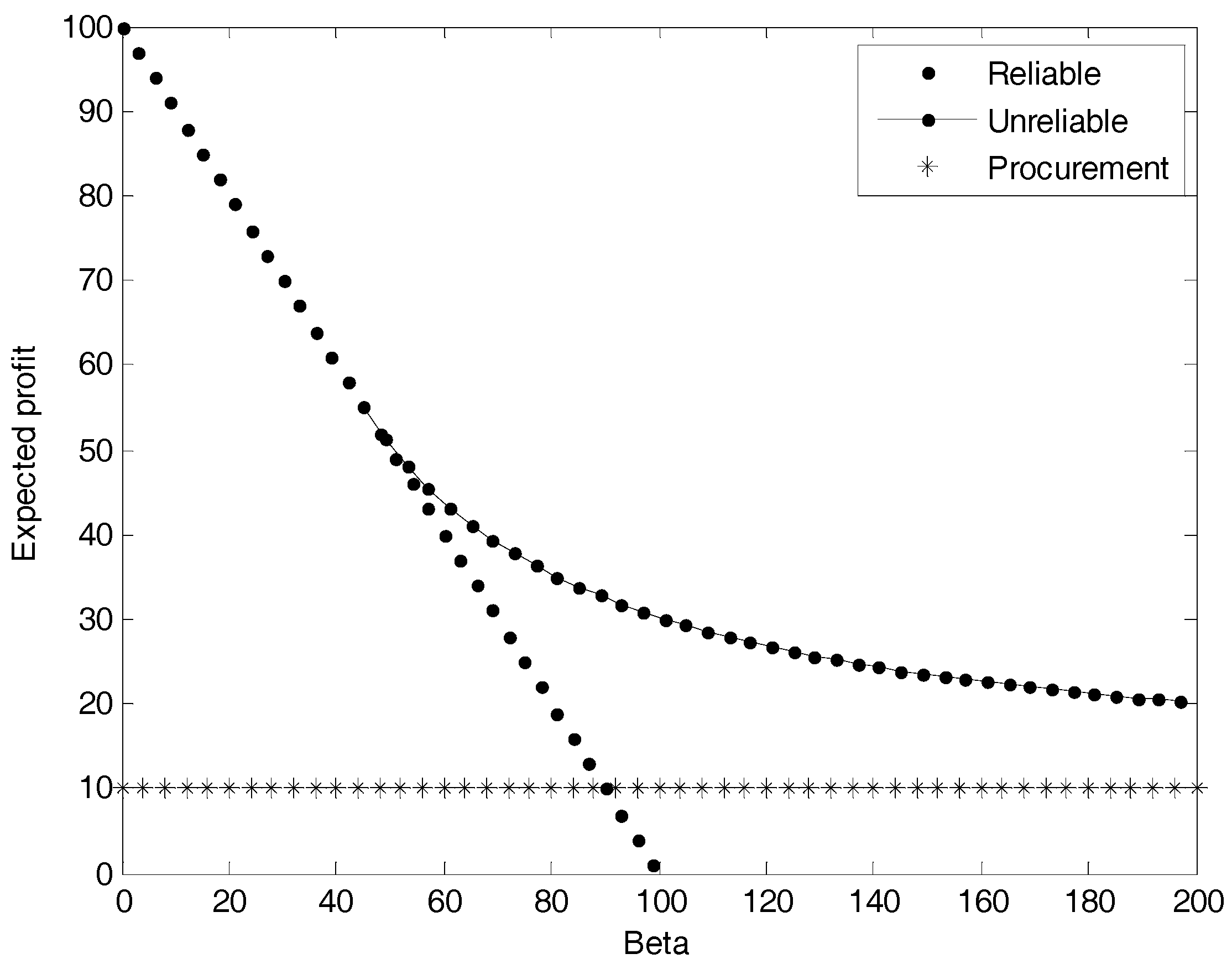
In Figure 2, the profit from emergency procurement is . When , supplier is more likely to be unstable. (1) When , the cost coefficient is small, the supplier can be completely stable or unstable. In this case, choose to be completely stable is better than direct emergency procurement. Meanwhile, high stable level generates high cost to the supplier, then the supplier would choose to be less stable to get more profit. Moreover, when the cost coefficient increases, (see Proposition 6) would increase, less stable would be better for the supplier. Then the retailer would not increase the purchasing price; (2) when , the cost is high. Since the market demand is limited, the retailer will not increase ordering quantity. The retailer would increase the purchasing price. When the purchasing price is no less than the emergency purchasing price, the supplier would be completely stable and the emergency procurement would be better than complete stable strategy. However, the high emergency procurement price would make the profit of emergency procurement less than the expected profit of the supplier when it is not stable, so the retailer would make the supplier to be less stable.
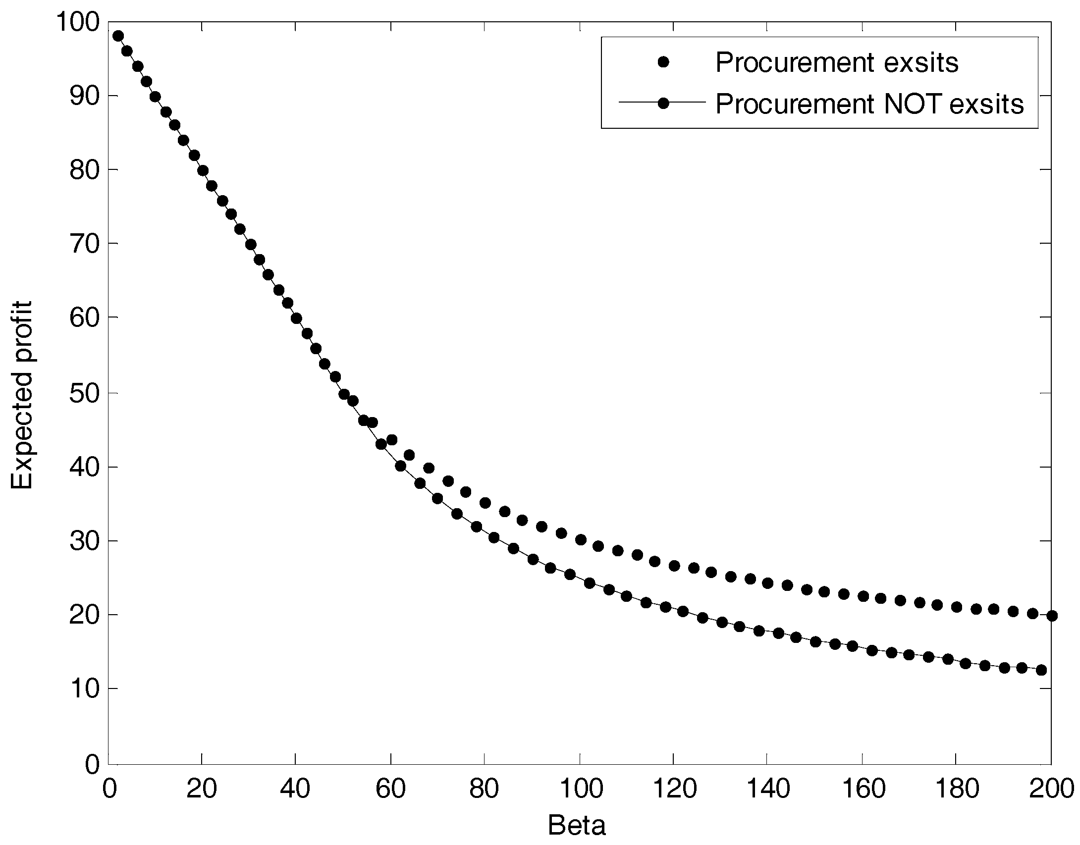
When the purchasing price increases more, the threshold will increase accordingly. This means that high purchasing price makes the retailer unwilling to purchase during the disruption, even if it is costly for the supplier to be more stable. The retailer would increase the procurement price to make the supplier more stable. In the very extreme case, when , i.e., the emergency purchasing price equals to the retail price, the retailer can’t get any profit through emergency procurement. Recall that in Case 4 where the emergency procurement does not exist. From Corollary 1 and Figure 4, we know that the retailer still can get non-negative profit through a properly selected procurement strategy. After comparing the case with emergency procurement strategy and the case without emergency procurement strategy, we find that: the retailer would prefer to improve the stability if there is no emergency procurement strategy. However, the expected profit would decrease accordingly. This implies that emergency procurement strategy is an efficient way to reduce the risk of supply disruption.
6. Extended Model
In the above analysis, we assume that the stability level of suppliers is related to the procurement strategies of retailers and the unit cost of a certain product will not change during the whole process. However, it should be noted that the variable part of unit cost which defines as the sum of variable costs among production, transportation and assembly may lower with the increasing of fixed inputs and the advancement of stability level. For example, based on data analysis on hard disk drive manufacturing, Bohn and Terwiesch [10] found out that if the output value increased by 8 percentages, the unit labor contribution would subsequently rise by 20 dollars, thus they proposed that increasing output can reduce costs. Another instance was the application of RFID technology, which realized the track management during the process of production and directly cut down the expenditures for quality control [28]. Furthermore, this technique also simplified the procedures of transportation and assembly, and therefore decreasing transport and labor expenses [28]. Given this, we consider the impact of stability level on variable costs in extended model by proposing that the rising of stability level contributes to the reduction of unit variable cost. Similar to most literatures regarding product or process innovation [26,29], we treat the fixed inputs as the efforts to lower the variable costs and assume that the reduction of unit variable costs is the concave function of the fixed inputs, which means margin utility decreases as fixed inputs increase. In summary, we mainly discuss how the reduction of variable costs resulted from fixed inputs affects strategy selection of suppliers and retailers.
In extended model, we only add an assumption on the basis of original model: the unit cost is the linear function of the stability level. More specifically, we propose that with the input of technology, the stability level of suppliers will increase while the unit cost will drop. Generally, a number of studies have confirmed that the unit cost is negatively related to investments and stability. For instance, Heese and Swaminathan [29] pointed out that sufficient design investments can lower the expenditure in manufacturing and the marginal utility of inputs is declining. Referring to this finding, we assume that the marginal reduction of unit variable cost is less than the marginal increment of fixed inputs, and the input cost is the function of the reduction of unit variable cost (this situation can be explained by the same reasons used in Proposition 2). Consequently, we consider that the reduction of unit variable cost is the linear function of the stability level.
6.1. The Optimal Stability Level
Based on original assumptions and the additional condition, we can get the profit function of suppliers as follows:
where is cost coefficient, and it is obvious that when suppliers are entirely stable (), the fixed inputs is ; is unit variable cost of certain products provided suppliers are entirely stable; c is the margin of the unit variable cost to the stability level. Hence, in order to achieve profit maximization, the optimal stability level of suppliers should satisfy the following proposition.
Proposition 7.
The optimal stability of suppliers is
From Formula (12) we can see that the cost coefficient represents the difficulty degree of suppliers to capture stability. Besides, the increasing of order quantity and procurement price can both encourage the rising of suppliers’ stability, indicating the substitutability between those two factors. This is because, once the deliveries match the requirement of retailers, more orders and higher price stand for greater profits. Meanwhile, acting as procurement price, marginal cost c plays a positive role to the stability level. Consequently, it is easier for suppliers to keep stable when considering the interaction between stability level and unit cost.
6.2. The Optimal Order Strategy
The profit of retailers is consistent with newsvendor model [30,31], and we can get the profit function based on Formula (1) and (2) as follows:
Thus, the expression of expected profit is:
where is just explained in Formula (12); I is the distribution interval of demand; stands for the supremum of demand.
In the extended model, retailers make a compound decision for order quantity and procurement price considering the stability level of their suppliers. There are two strategies for retailers: firstly, when , in this case suppliers are entirely stable while the input cost of retailers is higher; secondly, when , in this condition, the supply is unstable and has the possibility to break off. In term of the form of Formula (12), the Formula (14) is a question of higher bivariate extreme. Given this, we hold the proposition as follows:
Proposition 8.
- (i)
- When the order satisfies the condition of , the supply is entirely stable, and the expected profit is the concave function of the order quantity;
- (ii)
- When the order satisfies the condition of , the expected profit is the concave function of the procurement price.
In Proposition 8, we analyze retailers’ expected profit function as well as its concavity and convexity under the two strategies, which provide great guidance for solving the optimal procurement strategy. To obtain analytical solution, we assume that the market satisfies uniform distribution, namely ; then we can get , and .
Proposition 9.
If , then the suppliers tend to be entirely stable.
- (1)
- When , ;
- (2)
- When , , then , ;When , , then , ;When , , then the retailers will not order;
- (3)
- When , then , ;
- (4)
- When , then the retailers will not order.
The Proposition 9 provides the optimal procurement strategy of retailers under the condition of . In situation (1), the expected profit is , in situation (2), the expected profit is , in situation (3), the expected profit is . Meanwhile, when the value of (cost parameter) is over a certain threshold (namely ), retailers will not encourage suppliers to be entirely stable. Moreover, compared with the condition where does not exist, the threshold value in extended model increases, which means the willingness of retailers to motivate suppliers’ stability rises as well.
Proposition 10.
When ,
- (1)
- When , then , ;
- (2)
- When , if , then , ; if , then , the retailers will not order.
The Proposition 10 offers the optimal procurement strategy of retailers under the condition of . In situation (1), the expected profit is ; in situation (2), the expected profit is . According to the comparison of maximum expected profits in different conditions, we acquire the optimal procurement strategy of retailers and optimal stability level of suppliers as follows:
Proposition 11.
- (i)
- When , then , , ;
- (ii)
- When , if , then , , ; if , retailers will not order, however, provided , then , , .
As it shows in Proposition 11, with the increasing of , the optimal order quantity rises while the optimal procurement price drops. This is because the reduction of unit variable cost resulted from stability improvement has the similar utility with procurement price, thus retailers tend to enlarge order quantity but decrease procurement price. When cost coefficient is under a certain threshold, suppliers verge to entire stability; when cost coefficient is above this threshold and the emergency procurement price is relatively high, then suppliers hardly tend to be stable. However, it should be noted that when emergency procurement price is relatively low, the procurement strategy is complex. Firstly, if the cost coefficient is slightly over the threshold, then retailers will directly make emergency procurement due to the low price (); next, with the increase of cost coefficient, retailers believe that a higher () will motivate suppliers to be firmly stable; finally, when the coefficient rises too high, retailers will discard the order with the consideration of suppliers’ cost.
7. Conclusions
In this paper, we intend to construct a dynamic model to analyze retailer’s procurement strategy when supply stability is endogenously determined. We attempt to characterize the optimal supply stability and the optimal purchasing strategy by using a quadratic cost function. Based on these models, we hold the following findings. Firstly, when the difficulty level of building supply stability exceeds a certain threshold, it would be more profitable for the retailer to choose a less reliable supplier. Secondly, given that the suppliers can get positive profit, the retailer would choose the one who has the strongest ability to be reliable. Thirdly, the equilibrium supply to the retailer would always meet the demand on the retailing market. Finally, we try to show that emergency procurement is an effective way to reduce the risk of supply chain disruptions. To better fit the real situations, an extended model which considers the impact of the stability on costs is further discussed. According to the extended model, we can also find a higher threshold which is similar to that in the first situation, indicating that retailers’ motivation to encourage suppliers to be entirely stable rises in this scenario. Besides, the optimal order quantity is positively related to parameter , while the optimal purchasing price is negatively related to parameter , which means, when encouraging the stability, retailers tend to increase the order quantity and decrease the purchasing price. In addition, the emergency procurement strategies of retailers are influenced by emergency procurement price and cost coefficient.
Our study can also be extended in future studies. For instance, the supplier might improve the technology to reduce the cost of production [32]. One example is the adoption of the automatic production line with radio frequency identification (RFID) technology which improves the stability of the supply level; at the same time, the RFID technology can also reduce the production cost [33]. Meanwhile, retail prices could also affect the market demand [34]. All these questions can be studied in the extension of our model.
Supplementary Files
Supplementary File 1Acknowledgments
The authors are greatly indebted to Cao and Yang for their valuable comments on the earlier draft of this paper. Moreover, the authors wish to thank National Planning Office of Philosophy and Social Science (CN) for funding this research with the Major Project of the National Social Science (No. 11&ZD165).
Author Contributions
Chengxiao Feng conceived the original research model; Zhenyu Jiang performed the analysis of the original model and proposed the extended model; Zongjun Wang performed the numerical analysis.
Conflicts of Interest
The authors declare no conflict of interest.
Appendix A
Appendix A.1. Proof of Proposition 4
(1) We assume that the distribution is uniform, and then according to Case 1, we can get the expression of expected profit which is only related to procurement price as follows:
Setting , (), thus and are the roots of ; the domain of definition of Formula (A1) is . It is easy to find that expected profit decreases in the interval of , thus the optimal procurement price is , and the optimal order quantity is . Due to , namely , then substituting it into Formula (A1), we can get the optimal expected profit is .
(2) Based on Case 2, we can get the expression of expected profit as follows:
Setting , then Formula (A2) can be transformed as:
The first derivative is . Obviously, Formula (A3) is an increasing function in the interval of , and a decreasing function in the interval of . Here we make a deep analysis on Formula (A3).
If , , then , and when , we can get . In addition, due to , namely and , thus we can get , .
If , , then . When , , we can get , namely , ; when , , we can obtain , namely , . In this condition, procurement price equals to emergency procurement price, and the optimal order quantity overrun the upper limit of predicted market demand, thus retailers tend to adopt emergency procurement instead of ordering goods.
Consequently, when , and , , the optimal expected profit is . Because the cost coefficient is too high, retailers will not take any measures to encourage suppliers to be entirely stable.
Combining (1) and (2), we can get to know , which means when , is also the optimum. To sum up, when , and , , the optimal expected profit is ; when , the suppliers cannot verge to complete stability.
Appendix A.2. Proof of Proposition 5
First, the order quantity should satisfy the condition of .
(1) According to Case 3, the expression of expected profit which is only related to is:
Setting , , , thus and are the roots of ; the domain of definition of Formula (A4) is . Taking the derivative of , we have , which indicates that expected profit increases in the interval of , decreases in the interval of , and reach the maximum when . However , thus the optimal order quantity is , and the corresponding procurement price is . In this situation , therefore the procurement strategy is the same as that in Proposition 4, and we can get .
(2) Based on Case 4, we can get the expression of expected profit as follows:
The first derivative is , indicating it is an increasing function in the interval of and a decreasing function in the interval of . Here we make a deep analysis on Formula (A5).
If , , then we have , , and the expected profit is .
If , , we can prove that . Because and satisfy the equation , thus it is easy to know . Substituting it into Formula (A5), we can obtain that the expected profit is . Consequently, we have , , or , . In this occasion , suppliers are entirely stable.
By comparison, when , we can get , thus meet this situation.
Appendix A.3. Proof of Proposition 7
Taking the derivative of Formula (1), we can know that satisfy the function. This completes our proof.
Appendix A.4. Proof of Proposition 8
(i) When , we have , and the expected profit of retailers is:
where , and we take the first and the second partial derivative of order quantity:
(ii) Similarly, when , retailers’ expected profit and its partial derivative are:
According to Formula (A8) and (A11), we can easily acquire the concavity and convexity.
Appendix A.5. Proof of Proposition 9
In this situation , let Formula (6) equals to zero, we can get , and from the (i) in conclusion (2), we have . The classified discussion is done as follows.
(1) if , then , thus it must have . Substituting it into, we can get the expression of expected profit only related to wholesale price as follows:
Because , we know that Formula (A12) is a decreasing function in the interval of . Setting , , then the domain of definition is . When , , it is obvious to know ; when , , we have , and due to , then the expectation is in this situation.
(2) if , namely , , then the expectation is:
Taking the replace of , then , and the expression of expected profit related to is:
Its first derivative of v is , thus the function increases in the interval of and decreases in the interval of .
(i) when , , then .
If , then , the function decreases; we can also get , , , indicating the wholesale price equals to emergency procurement price, thus retailers will not order.
If , then , we have , and therefore , .
If , then , thus it is easy to know , .
(ii) when (namely ), , then the domain of definition is , thus we can know , and .
If , then , the function increases; we can also get , , thus this situation should be rejected.
If (), namely , then , , ; when , , the function is increasing, and , .
(iii) when , we have , then , namely , however, there is , thus the function is increasing, and , , .
According to Formula (A13), we can know that in situation (ii) and (iii), when , the expectation is ; in situation (iii), when , the expectation is . Moreover, within the overlapping interval () of situation (ii) in (1) and (2), there is . This completes our proof.
Appendix A.6. Proof of Proposition 10
In this situation, , letting Formula (9) equals to zero, then we have . Combining the (ii) with conclusion (2), we can know . First, it should satisfy the condition of , namely . Setting , and then we take classified discussion as follows.
(1) if , namely , then there is . In this condition, the expression of expectation profit only related to order quantity is:
It is obvious that this function increases provided , and decreases provided . Meanwhile, its domain of definition is , and there is , thus we can obtain , and .
(2) if , namely , then the expected profit is:
Its first derivative is , indicating the function increases in the interval of and decreases in the interval of .
(i) when , ,
If , namely , then we have , ; if , namely , then we have , .
(ii) when (there is ),
If , namely , then we can get ; if , namely , then we have , .
(iii) when , then we can know , , thus .
According to Formula (A16), in situation (i) where , the expected profit is ; in situation (ii) and (iii), the expected profit is . By comparing these two expectations, we can know , thus case (1) is satisfied under the condition of .
Appendix A.7. Proof of Proposition 11
We compare the expected profit of conclusion (3) with (4) in different interval.
(1) when , we have , thus get ;
(2) when , there is , thus it is ;
(3) if , then when , , thus it is ; if , then retailers do not order when , but they get when .
References
- Muthukrishnan, R.; Shulman, J.A. Understanding supply chain risk: A McKinsey global survey. McKinsey Q. 2006, 9, 1–9. [Google Scholar]
- Banker, S. Volcano Disrupts European Supply Chains. Logistics Viewpoints, 2010. Available online: http://logisticsviewpoints.com/2010/04/22/volcano-disrupts-european-supply-chains (accessed on 4 December 2017).
- Veysey, S. Majority of Companies Suffered Supply Chain Disruption in 2011: Survey. Business Insurance, 2011. Available online: http://www.businessinsurance.com/article/20111102/NEWS06/111109973# (accessed on 4 December 2017).
- Heyes, W. Honest Broker Solves Supply Problems. 2008. Available online: http://www.epdtonthenet.net/article.aspx?ArticleID=14675 (accessed on 4 December 2017).
- Hu, X.; Gurnani, H.; Wang, L. Managing risk of supply disruptions: Incentives for capacity restoration. Prod. Oper. Manag. 2013, 22, 137–150. [Google Scholar] [CrossRef]
- Tomlin, B. On the value of mitigation and contingency strategies for managing supply chain disruption risks. Manag. Sci. 2006, 52, 639–657. [Google Scholar] [CrossRef]
- Liker, J.K.; Choi, T.Y. Building Deep Supplier Relationships. Available online: https://hbr.org/2004/12/building-deep-supplier-relationships (accessed on 4 December 2017).
- Gümüş, M.; Ray, S.; Gurnani, H. Supply-side story: Risks, guarantees, competition, and information asymmetry. Manag. Sci. 2012, 58, 1694–1714. [Google Scholar] [CrossRef]
- Krause, D.R.; Handfield, R.B.; Tyler, B.B. The relationships between supplier development, commitment, social capital accumulation and performance improvement. J. Oper. Manag. 2007, 25, 528–545. [Google Scholar] [CrossRef]
- Bohn, R.E.; Terwiesch, C. The economics of yield-driven processes. J. Oper. Manag. 1999, 18, 41–59. [Google Scholar] [CrossRef]
- Mendoza-Fong, J.R.; García-Alcaraz, J.L.; Díaz-Reza, J.R.; Sáenz Diez Muro, J.C.; Blanco Fernández, J. The role of green and traditional supplier attributes on business performance. Sustainability 2017, 9, 1520. [Google Scholar] [CrossRef]
- Federgruen, A.; Yang, N. Technical note-procurement strategies with unreliable suppliers. Oper. Res. 2011, 59, 1033–1039. [Google Scholar] [CrossRef]
- Liu, S.; So, K.C.; Zhang, F. Effect of supply reliability in a retail setting with joint marketing and inventory decisions. Manuf. Serv. Oper. Manag. 2010, 12, 19–32. [Google Scholar] [CrossRef]
- Gurnani, H.; Shi, M. A bargaining model for a first-time interaction under asymmetric beliefs of supply reliability. Manag. Sci. 2006, 52, 865–880. [Google Scholar] [CrossRef]
- Tomlin, B. Impact of supply learning when suppliers are unreliable. Manuf. Serv. Oper. Manag. 2009, 11, 192–209. [Google Scholar] [CrossRef]
- Wang, Y.; Gilland, W.; Tomlin, B. Mitigating supply risk: Dual sourcing or process improvement? Manuf. Serv. Oper. Manag. 2010, 12, 489–510. [Google Scholar] [CrossRef]
- Tang, S.Y.; Gurnani, H.; Gupta, D. Managing disruptions in decentralized supply chains with endogenous supply process reliability. Prod. Oper. Manag. 2014, 23, 1198–1211. [Google Scholar] [CrossRef]
- Loseby, M. Vertical Coordination in the Fruit and Vegetable Sector: Implications for Existing Market Institutions and Policy Instruments; OECD: Paris, France, 1997. [Google Scholar]
- Yan, M.R.; Chien, K.M.; Yang, T.N. Green component procurement collaboration for improving supply chain management in the high technology industries: A case study from the systems perspective. Sustainability 2016, 8, 105. [Google Scholar] [CrossRef]
- Xue, X.; Wang, S.; Lu, B. Computational experiment approach to controlled evolution of procurement pattern in cluster supply chain. Sustainability 2015, 7, 1516–1541. [Google Scholar] [CrossRef]
- Lee, H.; Lodree, E.J. Modeling customer impatience in a newsboy problem with time-sensitive shortages. Eur. J. Oper. Res. 2010, 205, 595–603. [Google Scholar] [CrossRef]
- Kim, S.H.; Tomlin, B. Guilt by association: Strategic failure prevention and recovery capacity investments. Manag. Sci. 2013, 59, 1631–1649. [Google Scholar] [CrossRef]
- Li, G.; Zhang, L.; Guan, X.; Zheng, J. Impact of decision sequence on reliability enhancement with supply disruption risks. Transp. Res. Part E Logist. Transp. Rev. 2016, 90, 25–38. [Google Scholar] [CrossRef]
- Yan, R.; Lu, B.; Wu, J. Contract coordination strategy of supply chain with substitution under supply disruption and stochastic demand. Sustainability 2016, 8, 676. [Google Scholar] [CrossRef]
- Moorthy, K.S. Market segmentation, self-selection, and product line design. Mark. Sci. 1984, 3, 288–307. [Google Scholar] [CrossRef]
- Desai, P.; Kekre, S.; Radhakrishnan, S.; Srinivasan, K. Product differentiation and commonality in design: Balancing revenue and cost drivers. Manag. Sci. 2001, 47, 37–51. [Google Scholar] [CrossRef]
- Hill, T. Manufacturing Strategy, 3rd ed.; McGraw-Hill/Irwin: Boston, MA, USA, 2000. [Google Scholar]
- Xu, J.R.; Chen, J.S.; Niu, J.H. RFID and its application. Data Commun. 2009, 30, 21–26. (In Chinese) [Google Scholar]
- Heese, H.S.; Swaminathan, J.M. Product line design with component commonality and cost-reduction effort. Manuf. Serv. Oper. Manag. 2006, 8, 206–219. [Google Scholar] [CrossRef]
- Dada, M.; Petruzzi, N.C.; Schwarz, L.B. A newsvendor’s procurement problem when suppliers are unreliable. Manuf. Serv. Oper. Manag. 2007, 9, 9–32. [Google Scholar] [CrossRef]
- Tomlin, B.; Wang, Y. On the value of mix flexibility and dual sourcing in unreliable newsvendor networks. Manuf. Serv. Oper. Manag. 2005, 7, 37–57. [Google Scholar] [CrossRef]
- Das, T.; Krishnan, V.; McCalley, J.D. High-fidelity dispatch model of storage technologies for production costing studies. IEEE Trans. Sustain. Energy 2014, 5, 1242–1252. [Google Scholar] [CrossRef]
- Delen, D.; Hardgrave, B.C.; Sharda, R. RFID for better supply-chain management through enhanced information visibility. Prod. Oper. Manag. 2007, 16, 613–624. [Google Scholar] [CrossRef]
- Sekizaki, S.; Nishizaki, I.; Hayashida, T. Electricity retail market model with flexible price settings and elastic price-based demand responses by consumers in distribution network. Int. J. Electr. Power Energy Syst. 2016, 81, 371–386. [Google Scholar] [CrossRef]
Figure 1.
Interaction between the retailer and the supplier (Stackelberg game).
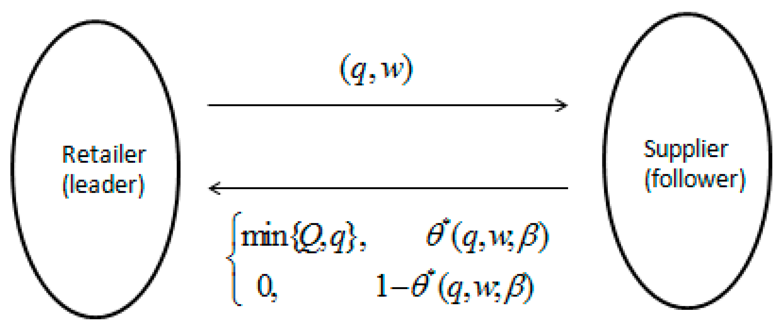
Figure 2.
Optimal expected profit with different .

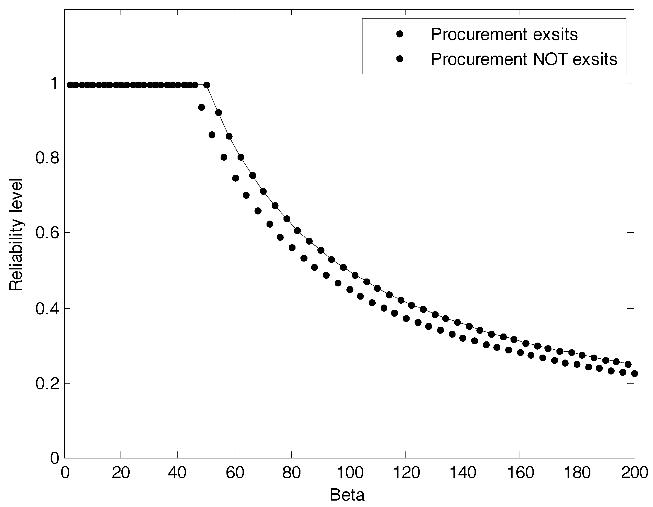
Figure 3.
The impact of on supplier’s reliability level.

Figure 4.
The impact of procurement strategy on supplier’s expected profit.

Table 1.
Optimal procurement strategy and reliability level under normal distribution.
| Cost-Efficient | Reliability Level | Quantity | Wholesale Price | Expected Profit |
|---|---|---|---|---|
| 16 | 1 | 12 | 1.4 | 116.390 |
| 31 | 1 | 14 | 2.5 | 99.358 |
| 66 | 1 | 12 | 5.5 | 73.895 |
| 91 | 0.77143 | 13 | 5.4 | 56.570 |
| 146 | 0.45959 | 11 | 6.1 | 40.108 |
| 211 | 0.31280 | 12 | 5.5 | 32.427 |
| 246 | 0.29593 | 13 | 5.6 | 29.432 |
| 276 | 0.27899 | 14 | 5.5 | 27.733 |
| 281 | 0.25907 | 13 | 5.6 | 27.679 |
| 336 | 0.22321 | 15 | 5.0 | 24.762 |
| 356 | 0.19719 | 13 | 5.4 | 24.539 |
| 376 | 0.17287 | 13 | 5.0 | 23.543 |
| 391 | 0.17187 | 12 | 5.6 | 23.049 |
| 416 | 0.15817 | 14 | 4.7 | 23.011 |
| 461 | 0.14317 | 12 | 5.5 | 21.674 |
| 496 | 0.13065 | 12 | 5.4 | 21.615 |
© 2017 by the authors. Licensee MDPI, Basel, Switzerland. This article is an open access article distributed under the terms and conditions of the Creative Commons Attribution (CC BY) license (http://creativecommons.org/licenses/by/4.0/).
Share and Cite
MDPI and ACS Style
Feng, C.; Wang, Z.; Jiang, Z. Retailer’s Procurement Strategy under Endogenous Supply Stability. Sustainability 2017, 9, 2261. https://doi.org/10.3390/su9122261
AMA Style
Feng C, Wang Z, Jiang Z. Retailer’s Procurement Strategy under Endogenous Supply Stability. Sustainability. 2017; 9(12):2261. https://doi.org/10.3390/su9122261
Chicago/Turabian StyleFeng, Chengxiao, Zongjun Wang, and Zhenyu Jiang. 2017. "Retailer’s Procurement Strategy under Endogenous Supply Stability" Sustainability 9, no. 12: 2261. https://doi.org/10.3390/su9122261
Note that from the first issue of 2016, this journal uses article numbers instead of page numbers. See further details here.