1. Introduction
Local Public Administrations (LPAs) have the responsibility of providing high quality, cost-efficient and sustainable public services to their citizens. The growing interest displayed by politicians and researchers alike, towards public expenditures’ efficiency, is needed and welcomed. Locally-elected representatives need to promote and facilitate social and economic development, efficient territorial organization and supply easily reachable and sustainable quality public goods and services, such as: communal services and public order, social protection, modern sewage and water treatment, public transportation, education and health services, cultural and leisure services, environment protection and water distribution, to name just a few. It is highly desirable that such local public services be provided efficiently and sustainably in terms of timely delivery, costs and quality, especially in countries where corruption, bureaucracy, social indifference and economic development are still a great matter of concern.
Efficiency in the public sector refers to the optimal use of resources in view of maximizing public goods and services’ output. One economic system is more efficient than the next when it offers a bigger supply of public goods and services without consuming a higher amount of resources [
1] (pp. 13–18).
The term sustainable public goods and services represents a particular form of the more general concept of sustainable public finances or public sector performances. A central issue of the Maastricht Treaty is that a successful European Union requires sustainable public finances for its member states. Yet, there was no clear definition of sustainability in this area. The economists’ common use of the term builds on the concept of budget constraint over an infinite time horizon, which is of little practical use. There are far too many ways in which fiscal policies can comply with a budget constraint encompassing infinite periods, and for practical purposes, the concept itself is not very useful [
2] (p. 8).
Throughout this study, we develop a concept of sustainability focusing on the relationship between financial resources derived from taxpayer’s contributions and the results obtained and quantified through different selected services provided at the local level.
Sustainability and efficiency are closely related in the context of the public sector, as sustainability also implies that human needs are fairly and efficiently satisfied. This objective requires that elected officials and politicians, along with nonprofit community organizations, business class and, of course, citizens should be engaged in enforcing such a democratic objective and change policies, programs and practices into sustainable ones. Nonprofit community organizations, local and central government representatives and private sector companies participating in public tenders should make any effort to work together and organize different actions to show citizens and other parties the best practices in public sustainability and to demonstrate how these meet their needs.
The public expenditures’ analysis may validate or not citizens’ perception that public resources are not always used according to the principles of sustainability, efficiency, efficacy and economy. Such principles, along with general financial published data, allow residents of any given community to access the information needed to effectively monitor and control their political representatives’ activity. Consequently, LPAs should be motivated to act efficiently to secure the interests of local collectivities. Furthermore, they should become aware of the increased role they play in providing communities with sustainable goods and services and contribute to the increased momentum of the decentralization process.
In this context, competition between various territorial-administrative units may appear. Tiebout (1956) argues that increased competition between those administrations is beneficial as public services’ supply tends to become Pareto-efficient [
3]. Nevertheless, other economists [
4,
5,
6] (Schwab and Oates 1991; Davis and Hayes 1993; Krueger 1999) pinpointed the influence that other factors besides the fiscal ones (e.g., individual features and the expectations of each and every individual of that jurisdiction) may have upon public goods’ supply and competition between administrations. These economists proved, using different models, that decentralization alone cannot guarantee the optimization of satisfaction for heterogeneous collectivities.
At a global level, access to quality public and social services is essential for daily life, economic and social wellbeing. Efficiency and sustainability are essential to make sure the beneficiaries receive the best possible services, corruption is minimized and the local economy can benefit.
In the United States, Mildred E. Warner performed extensive research on the provision of public and community services, their financing and sustainability. The author studied the private financing of social programs via social impact bonds (SIBs) and found that the latter failed to attract private market investors without substantial additional guarantees (Warner, 2013). Furthermore, the author stated that SIBs raise questions about government’s ability to ensure broader public values [
7].
Warner and Hefetz (2012) found that in the U.S., public insourcing (reverse contracting) was roughly equal to the level of new outsourcing to private operators for the 2002–2007 period. The authors have studied the way city managers decide to privatize services or even reverse their privatization, analyzing survey data regarding service delivery for 67 local government services [
8].
In the European case, the Europe 2020 Strategy, the Lisbon Reform Agenda and the Stability and Growth Pact call for enhancing the quality and efficiency of services provided to citizens and consumers. According to Di Meglio et al. (2015), the provision of public services accounts for almost 25% of the value added and 33% of employment across the European Union, and as such, assessing the performance of these activities is a matter of interest in its own right and the result of the indirect influences they have upon the economy [
9].
In the European context, adequate provision of public services is an essential pillar of social cohesion, which has multiple dimensions inside the European Union. One important focus of EU policy is territorial access. Clifton et al. (2015) found that citizens are not uniformly satisfied with public service provision, with urban citizens being on average more satisfied than rural ones. Public services should be provided to all citizens, regardless of their socio-economic differences [
10]. However, the same authors proved one year before that more vulnerable citizens are less satisfied than their peers in regard to the public services provided to them by national and local government [
11].
Inter-municipal cooperation in delivering public services was studied by Bel and Warner (2015). Using a meta-regression analysis, the authors found strong evidence that fiscal constraints, spatial and organizational factors are significant drivers of cooperation between municipalities [
12].
Ferrari and Manzi (2014) found that citizen assessments or surveys, typically in the form of quality or satisfaction ratings, are frequently used to measure the performance of public services and advise public managers on how to improve citizens’ satisfaction [
13].
Romania, an EU member since 2007, is committed to complying with the directives of the European Union’s agenda in this field, while it is still confronting corruption and inefficiency in using public resources. Its citizens are demanding increased efficiency and transparency in the provision of public services and goods.
In our paper, we evaluate public expenditures’ efficiency for Romania’s 41 counties and Bucharest municipality, using the Data Envelopment Analysis (DEA) mathematical model. Our main purpose is to identify the efficient counties under different assumptions, respectively one input, six outputs and one input, one output, to publish the results and to determine improvements from the least efficient counties for the benefit of their citizens. Furthermore, we wanted to assess whether variables, such as a county’s number of inhabitants, and the level of inputs influence the outputs in a significant way.
We consider that our research brings a substantial contribution to this field’s literature by supplying new evidence and aspects regarding LPA expenditures’ efficiency. This becomes more important and relevant in the context of decentralizing policies designed to refocus public decision-making from central to lower levels of government.
Papers studying local spending efficiency and local services sustainability are not (very) abundant in the economic literature. Moreover, we could not identify studies done for Romania or other developing countries in which DEA or any similar mathematical instruments were used to analyze the relationship between financial efforts and the feedback/results the citizens receive via public goods and services. As such, even if the paper focuses only on one country’s set of local governments, its interest is not purely parochial, as local governments also account, even in different degrees, for a significant part of the general governments across the EU.
Another contribution of our paper is that we introduce a global output measure, called TCIO (Total County Output Indicator). It represents a similar measure to that of Afonso and Fernandes (2006), who developed in their studies TMOI (Total Municipal Output Indicator) and recommended it to be extended to other samples of local governments across the EU or abroad [
14]. As a consequence, our DEA analysis is performed both using all of the sub-indicators as outputs and alternatively with the composite TCIO.
Our research targets both decision-makers and citizens and tries to draw the attention upon the way public funds are spent in a context marked by public financial resources’ shortages and budgetary restrictions. We should also mention that the assessment of public services’ sustainability is an important issue, taking into account the role of local governments as major public employers and providers of a diversity of services. As Domingues et al. (2015), we consider that local governments are closer to citizens and respond faster than any other public sector level integrating sustainability principles in their operations and strategies [
15].
The structure of the remainder of our paper is as follows:
Section 2 emphasizes several theoretical aspects regarding the materials used and the mathematical method applied to process information: data envelopment analysis;
Section 3 presents the methodology used and the empirical results; discussions are to be found in the fourth part, whilst the fifth part concludes.
2. Materials and Methods
Barro (1990) assessed that an increase in public investments, hence of public expenditures, is very much needed to maximize economic growth in general and local collectivities’ wealth in particular [
16] (pp. 122–124). Such a model requires the increase of inputs in order to obtain an implicit increase of the results/outputs.
Afonso and Fernandes (2006) have elaborated performance measures for the public sector. They distinguished between public sector performances, defined as the results of public policies and public sector’s efficiency, generated from engaging public resources.
2.1. Local Development and Delivery of Local Public Services in Romania
As an EU member, Romania is subject to EU laws and regulations. This section briefly describes current Romanian territorial division and the delivery of local public services. Joining EU structures in 2007, Romania had to enforce the new requirements in order to improve LPAs activity and reduce as much as possible the economic, social and territorial disparities.
The European Commission developed the concept of regional policy as an investment policy. It encourages competitiveness, economic growth, job creation, improved quality of life and sustainable development. These investments support the delivery of the Europe 2020 strategy. Regional policy is also an expression of the EU’s solidarity concerning less developed countries and regions, concentrating funds in the areas where they can make the most difference.
Keeping these disparities would undermine some EU cornerstones, including its large single market and its currency, the Euro. During 2007–2013, the EU had invested a total of 347 billion Euros in European regions [
17].
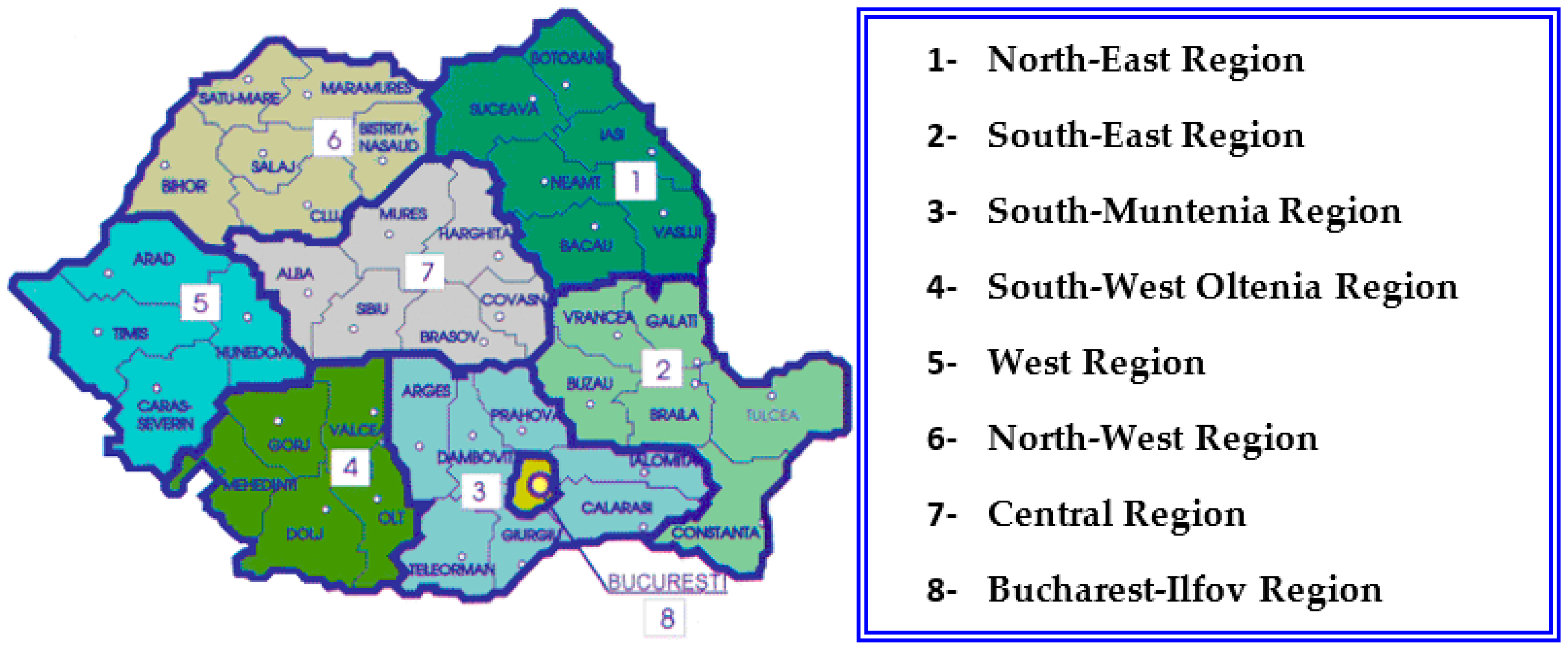
Romania uses the Nomenclature of Territorial Units for Statistics (NUTS), created by Eurostat with the purpose of offering a unique classification guide for EU regional statistics.
As mentioned, our study was based on data collected throughout 2011, from all 41 counties in Romania and Bucharest municipality. Each county contributes to the national budget and has its own budget, similar to cities and municipalities. Local budgets include local taxes, such as land tax, building tax, fees for advertising panels, as well as grants and amounts transferred from the central government budget.
Such territorial division involves relatively high functional costs, and it does not fulfil the efficiency requirements. Public administration reforms need to be carried out to reduce public expenditures and increase effectiveness and efficiency.
Conducting an administrative reform, issues such as administrative-territorial reorganization of Romania in regions of development are subject to intense debates, related to the efficient and sustainable decentralization of all public services of local interest. Although the eight regions of Romania are well known and precisely located, they do not have official legal recognition, being used mainly for statistical purposes [
18] (pp. 43–47).
In
Figure 1, we illustrate Romania’s counties and development regions.
A county represents an administrative-territorial unit, including municipalities, towns and communes, according to geographical, economic and socio-political criteria. The county assures the socio-cultural and municipal administration development of municipalities, towns and communes.
The idea of creating the eight regions materialized in 1998. The regions are administrative-territorial units, formed through the voluntary association of counties. Institutional framework, objectives and instruments of the regional development policy were revised in 2004, in the context of the negotiations in Chapter 21 Regional policy and structural instruments, by approving the regional development law in Romania [
19].
Romania’s territorial structure comprises 320 cities (municipalities and towns) and 2861 communes. These are basic administrative levels corresponding to NUTS Level IV. They are all part of the 41 counties, which, together with Bucharest, constitute NUTS Level III. Regions represent NUTS II, while the country, as a whole, is NUTS I.
Table 1 gives the total number of units as of 1 January 2016, according to the data published by the Romanian National Institute of Statistics.
The current territorial division encourages subordination of local authorities towards central government, an excessive dependence, which does not favor local initiatives. In this context, it is understandable why the EU asked for a new territorial division, where its policies could be applied. The new regions would be much larger, as seen in
Figure 1, and manage in a more responsible way the EU structural and cohesion funds.
In Romania, the institutions with responsibilities in this area are:
The National Council for Regional Development, a national partnership structure, with decision-making on the development and implementation of regional development policy objectives;
The European Integration Ministry, the institution designated to developing, coordinating, implementing and monitoring policies and strategies of regional development;
The Regional Development Council, a deliberative regional institution without legal personality, which functions in each region to coordinate different activities resulting from development policies;
The Regional Development Agency, a non-profit, legal personality body, promoting regional development.
In the European Union, the production and offer of local public goods and services should comply with the European Charter of Local Self-Government remarks. The Charter recommends applying basic rules to guarantee political, administrative and financial independence of local authorities. The principle of local self-government should be recognized in domestic legislation and, where possible, in the Constitution. Local representatives and authorities should be elected in universal suffrage.
Local authorities, acting within the limits of the law, will regulate and manage public affairs under their own responsibility, in the interests of the local population. Consequently, the Charter considers that public responsibilities should be exercised preferably by authorities closest to the citizens, the higher level being considered only when the co-ordination or discharge of duties is impossible or less efficient at the level immediately below. To this end, it sets out the principles concerning the protection of local authority boundaries, the existence of adequate administrative structures and resources for the tasks of local authorities, the conditions under which responsibilities at the local level are exercised, the administrative supervision of local authorities’ activities, the financial resources of local authorities and the legal protection of local self-government [
20].
Hence, for Romania, the LPA activity concerning the relation between public financial resources and public service delivery should comply with at least the following provisions of the European Charter:
LPA authorities have the right to keep their own revenues and to spend money freely in order to fulfil their tasks; this gives LPAs a degree of financial autonomy over revenue collection and public spending;
At least part of all financial resources should derive from local taxes (the level should be established by the LPA authorities within legal limits);
Offer protection to those units that encounter financial shortages by implementing some procedures to adjust the imbalance.
In very general terms, the sense of LPA expenditure autonomy is the right and ability of local governments to manage public property and funds in the interest of the local communities. The latter term implies that public resources are to be spent on goods and services to meet the demand of the local constituency. Therefore, first, local expenditure autonomy is equivalent with the freedom to decide which goods and services shall be financed from the local public budget and how much money shall be spent on each of them; second, expenditure autonomy also includes the freedom to decide how these goods and services shall be produced or delivered. With regard to both questions, autonomy also implies the ability of the local government to implement the decisions [
21] (p.73).
In 2009, Beer-Tóth argued that the distinction between expenditure responsibility (what to provide) and service delivery (how to provide it) is important. The assignment of a public expenditure function to a local government unit does not automatically mean that the latter will carry out all related tasks on its own. In the modern public sector, the production of goods and services is separated from the policy decisions concerning the choice of public services to be provided.
According to the Framework Law on Decentralization No. 195/2006, in Romania, among the activities lying exclusively in the responsibility of the LPA authorities, we may find [
22]:
The administration of local interest airports;
The administration of the county’s public and private field;
The administration of cultural institutions of local interest;
The administration of public health units of local interest;
Social care services for the victims of domestic violence;
Social care services for elderly persons.
Many of these responsibilities were included in our analysis as output or outcome measures.
2.2. Theoretical Approach of DEA Model
The concept of efficiency relies on the comparison method, and it describes a state of resource allocation in which it is not possible to have an efficient entity without identifying at least another entity deemed as inefficient. The efficient entity generates either the same output using a lesser amount of input or a higher volume of output using the same input [
23] (pp. 259–260). Starting from these premises, Farrell laid the foundations of the DEA model in 1957, which was later developed by Charnes, Cooper and Rhodes [
24].
The model was first applied in the United States in the education field as an analysis tool for the Follow Through Program [
25] (Rhodes, 1980). Subsequently, it was used in the healthcare, public economic sectors, banking and higher education sectors. This technique is widely used by both the public and the private sector, allowing the comparison of some parametric forms of the production functions, such as Cobb–Douglas.
In 2014, Cherchye et al. reconsidered the economic motivation of DEA by highlighting its behavioral interpretation [
26].
Still, DEA is more often applied to estimate the technical efficiency of the public sector’s decision units, defining their ability to produce public goods or to provide public services as near as possible to the convex efficiency frontier. The model can identify inefficient units amongst the studied ones, in which case the analysis continues revealing and explaining possible solutions for (in view of) generating better performances, ready to be adapted and implemented by the decision makers in order to reach a sustainable development for that community [
27,
28].
According to some authors [
29,
30], the relevance of the results and identifying the inefficient units is possible as long as for each input and output, there are at least three decision units included in the model. In 2001, Dyson et al. argued that the number of units should be at least double compared to the total number of inputs and outputs. These conditions allow the existence of a sufficient number of freedom degrees to implement DEA [
31]. Still, it is assumed that a too ample database could result in comparing ever more different units, hence more heterogeneous.
The DEA model is in essence a fractioned programming problem, as a ratio between a weighted outputs’ sum and a weighted inputs’ sum, in the case that the weights for inputs and outputs are selected to allow calculating the efficiency of the evaluated unit.
DEA assumes two working hypotheses: the first is based on inputs, by restricting the weighted outputs’ sum in order to minimize the inputs’ volume; whilst the second is based on the outputs’ level, restricting the weighted inputs’ sum in order to maximize the results [
32].
The approach of the model for linear convex portions in order to estimate the Farrell proposed frontier (1957) offers a non-parametric method to determine a unit’s relative efficiency as compared to the one of other similar decision units. The selection of an input- or output-oriented model is strictly dependent on the production process characterizing the decision unit. The two measurements lead to identical results for constants returns to scale (CRS) and different results for variable returns to scale (VRS).
Nevertheless, both the input and output-oriented models identify the same units as being efficient or inefficient.
Assuming we have
n Decision-Making Units (DMUs), each of them with m inputs and
s outputs, the unit’s p relative efficiency score is obtained solving the model proposed by Charnes et al. (1978) [
24]:
under
,
and:
where:
, the value of the k output produced by the i decision unit;
, the value of the j input used by the i decision unit;
, the weight of the j input, whereas , the weight of the k output.
The solving of Program (1) under the specified constraints (2) implies identifying those and values in order to maximize the i unit’s efficiency, provided that all of the efficiency levels are equal to one.
In order to avoid getting an infinite number of solutions, we also need (as well) to introduce the restriction:
Finally, we reach the following linear programming:
under
The linear program of maximization (4) and its restrictions (5) are known as the multiplying form of a linear programming problem [
33] (p. 9). The relations presented here can be used for n times to identify the efficiency scores for all of the n analyzed units. Each
i decision unit selects the weights of the inputs and outputs that maximize the efficiency score. A score below 1 denotes inefficiency. We have to mention that DEA is a primary diagnosis instrument, and it does not achieve decision units’ reconstruction strategies.
Should the output level increase proportionally, we have CRS. However, if the output measures modify at a slower pace compared to the input variables, then we get decreasing returns to scale, whereas if the output variables increase at a higher pace than the input variables, we get increasing returns to scale. These last two variants are specific to VRS.
2.2.1. Input-Oriented Measures
The following discussion and mathematical systems specific to the DEA method are illustrated both for CRS and VRS focusing on the input-reduction measurement.
As such, when we have a CRS DEA, the mathematical procedure is the following:
where:
θ, a scalar whose value obtained via Excel/other specialized programs (θ ≤ 1) reflects the efficiency of the i decision unit; the calculus of this scalar will be performed n times for each decision unit;
λ, a vector of positive constants of n × 1 size indicating the weight of the imposed restrictions;
θ and λ are variables whose values will change after processing the input and output data to observe the requirements imposed by the inequalities system;
Ykλ, a value determined for the n observed units as a sum of the products between the output value of the k variable and the vector indicating the specific weights; the procedure is then repeated for each k output variable (k = 1, 2, ..., s): sum product (Ykλ) or ;
yki, the output value of the k variable registered for the i unit;
Xjλ, a value determined for the n observed units as a sum of the products between the input value of the j variable and the vector indicating the specific weights; the procedure is then repeated for each j input variable (j = 1, 2, ..., m): sum product (Xjλ) or ;
θxji, the efficiency of the product between the θ scalar and the j input value registered for the i unit.
The CRS assumption is valid only when the researched units are operating at an optimal scale. The most frequent situations reveal that these units confront certain restrictions, especially of a financial kind or of imperfect competition, which induces them VRS, especially decreasing ones [
34] (p. 10).
In 1984, Banker et al. created an extension of the CRS DEA to explain VRS [
35] (p. 1078). Compared to the mathematical constraints of the CRS, the VRS adds the function convexity condition, respectively the weight constraints of each decision unit have to be equal to 1.
The inequalities system describing the constraints imposed by VRS DEA reads:
Should differences appear between the CRS and VRS generated technical efficiency for certain entities, it means they employ an inefficient scale, where the CRS use can be inappropriate since the units are not operating on an optimal scale.
2.2.2. Output-Oriented Measures
The above input-oriented technical efficiency measure addresses the question: “By how much can input quantities be proportionally reduced without changing the output quantities produced?” One could alternatively ask the question: “By how much can output quantities be proportionally expanded without altering the input quantities used?” [
36] (p. 6). This represents an output-oriented measure.
A VRS DEA model oriented toward the maximization of the output/outcome variables is described by the max function with the following constraints:
where:
Φ, a scalar whose value, obtained as a result of the Excel/other specialized programs processed data (1 ≤ Φ < ∞), will contribute to i decision unit efficiency’s determination and of the proportional increase that can be brought to output measures, maintaining constant the input level for each decision unit; the calculus of this scalar will be performed n times for each decision unit;
1/Φ, the efficiency score defining the below par level of technical efficiency (0 < 1/Φ ≤ 1);
Φ and λ, variables whose values are modified after processing the input and output data to comply with the requirements imposed by the inequalities system;
xji, the input value of the j variable registered by the i unit;
Φyki, the efficiency described by the product of Φ scalar and output value of the k variable of the i unit.
No matter the model’s orientation, both variants will estimate the same efficiency frontier; hence, they will identify the same set of efficient units. The scores associated with the inefficient units can be however different with θ < 1, respectively with Φ > 1.
Since the referential paper of Charnes, Cooper and Rhodes was published (1978), around 4500 ISI Web of Science DEA-related papers were published [
37].
2.3. Methodology
The evaluation and analysis of local public expenditures’ efficiency and services’ sustainability can be achieved assimilating public sector activities to a production process that transforms input such as labor and capital into outputs/outcomes [
38] (p. 186).
Frequently, direct output (D-output) variables cannot be calculated based on statistical published data, leading to their approximation via other relevant measures. In such cases, direct output (D-output) becomes an outcome (C-output), which presents an approximated result of the output variable. Often, this result is a much better reflection of the citizens’ felt satisfaction from that public service.
Our study concerns the year 2011, at the level of 41 Romanian counties and Bucharest municipality.
The measures for each of the 42 observations are studied relative to the ‘best-practice’ frontier. We find a similar approach regarding the evaluation and analysis of public expenditures in the case of Portugal. Using DEA, Afonso and Fernandes (2006) present an estimation of municipal spending’s extent considered ‘wasteful’ relative to the ‘best-practice’ frontier [
14] (pp. 40–43). Nevertheless, similar to our study, the two authors use DEA to compute input and output Farrell efficiency scores at the local level (still for a limited number of municipalities, 51 out of over 300 Portuguese municipalities) and for only one year (2001).
One of DEA’s many advantages, as a performance measurement technique, is allowing the use of input and output indicators at a certain moment in time. The lack of continuous or homogeneous data for certain output measures makes it very difficult or even impossible to build a multiyear analysis. We have chosen the fiscal year of 2011, as we found a comprehensive dataset for all 42 counties of Romania. 2011 was the year in which the Romanian population census took place, such that the demographic database used both for input and most output measures (expressed as average per capita) was closest to reality.
The research database includes 42 decision-making units, each of them with only one input, respectively local budgets’ expenditures, aggregated for each county, expressed as an average level per inhabitant (in Romanian national currency—
Lei/inhabitant) and six sets of outputs. Some output variables’ sets include more sub-measures, leading to a total number of 10 output variables. The output variables describe the analyzed public sector’s productivity and sustainability. The county data originate from Romanian National Institute of Statistics, consulting the statistical TEMPO-online databases [
39]. Some of the variables are
D-output, whilst others reflect the final result, being the
C-output type.
In
Table 2, we are presented the measures used for our research, while in
Table A1, from
Appendix A, we have all of the initial values of indicators and sub-indicators processed in this research.
With the variables from
Table 2, we aimed to cover as many types of public services as possible. We also wanted to introduce services provided and financed at a local level. Nevertheless, it is necessary to specify that for a significant number of public goods and services, the sub-national government does not have (has not) full authority, as they are not completely decentralized, especially in terms of monitoring and evaluating the observance of quality standards. The national mechanisms of supervision may limit both access to revenues (e.g., through taxes and social contributions, which although being collected at the territorial level, are part of the central government budget or by preventing LPAs from contract loans above a certain level established) and the way money is spent.
The 11 variables used as input and outputs are:
The input variable EXP/CAP for the local public expenditures per capita in terms of payments made by all of the counties, municipalities and towns, aggregated at each county level and expressed in the Romanian national currency (Lei/capita);
STABPOP D-output variable for the total stable population of each county (number of inhabitants) according to the results of the Population and Housing Census of 2011;
NPSEDU C-output variable that shows the proportion (%) of children 3–14 years of age attending nurseries or schools (primary and secondary) according to the Romanian National Institute of Statistics data upon education;
EPOP C-output variable gives the number of senior citizens and reflects the supply of municipal social services to the elderly population, such as home-based general assistance, retirement houses, etc.;
WATERPR C-output variable reflects the weight of population connected to public water supply/provision into the total population of each county (%);
WATERTR C-output variable shows the percentage of population connected to waste water treatment plants into the total population (%);
WATERSE C-output variable describes the weight of population connected to waste water collecting systems (sewerage) into the total population (%);
ACRELI C-output variable represents a culture measure, i.e., the number of active readers in libraries as the percentage of total population (%);
ENTICK C-output is the indicator showing how many tickets to a theater play, concert, etc., were sold as an average per county’s inhabitant (number of tickets/capita);
MODSTR C-output variable indicates the weight of modernized town streets’ length into total town streets’ length (%);
VERSPOTS C-output variable shows the weight of verdure spots’ areas into total municipalities and towns’ inside areas (%).
For our further analysis, we decided to group the ten output indicators into the six main types of public services presented in
Table 2. In order to aggregate the data, we need to homogenize the variables by standardizing their values. The results obtained analyzing the ten output sub-indicators are not very relevant, since some of them are part of the same type of public service offered by LPAs for local residents.
Expressing each measure’s values via indexes is one of the most common ways of processing the series of homogenous data. The procedure envisions standardizing each measure’s values around its average, such as every input and output’s average, to be equal to one. In this way, we can create a smaller number of output measures, grouped according to the local public service offered.
We have created a single output from the variables included in the public services of the public system of water supply (provision, treatment and sewerage), further called PSWS, culture and recreation (local libraries and entertainment institutions), further called CR, as well as the local interest public utility (modernized streets and environmental protection), further called LIPU. After analyzing the six output variables, the aggregation continues to obtain a single output variable (the unique output measure, TCIO) for all six measures, considering each holds an equal weight into the final output variable.
Standardizing the initial values requires two steps. The first stage calculates the arithmetic average values for each input and output. The second stage relates initial values for each county to the previously-established average. The indexes’ average value should be equal to one. Final values of the six output measures, as well as the results for the
TCIO variable are presented in
Appendix B,
Table B1.
3. Results
The performances of each county for the sub-measures presented in
Appendix A,
Table A1 suggest the existence of a significant standard deviation for the
CR variable. As compared to other variables, this indicator’s deviation from the average is the highest (1.3274). Counties displaying the most extreme values compared to the national average are Olt (with a very high index of 9.16), Suceava (1.75) and Sibiu (1.74). At the opposite pole, we find Giurgiu (0.32) and Constanta (0.40).
Significant deviations from the average values were also found for the general administrative public services, appreciated through the STABPOP (0.5651) and social services, appreciated by EPOP, the number of people aged 65 and above (0.5057). For these two variables, the farthest values from the average we can find for Bucharest (3.93 for administrative services, respectively 3.52 for social services addressed to elderly people).
The lowest standard deviation value is found for the variable basic education, expressed by the inclusion degree, NPSEDU (0.0569). The highest degree of inclusion can be found in Gorj county (1.08), whereas the lowest one is in Ilfov (0.74). The value for Ilfov is an exception at the national level, explained by the close vicinity to Bucharest city. For all other counties, this index has a value of at least 0.91.
PSWS and LIPU have the highest values in Bucharest (2.60, respectively 2.14). For the public services of water supply, water treatment and sewerage, good results are recorded also in Brasov (1.66), Cluj (1.65), Hunedoara (1.58), Constanta (1.56), Sibiu (1.46) and Timis (1.40).
Lower values we register in Ilfov (0.36), Giurgiu (0.48), Teleorman (0.53), Suceava (0.58), Olt and Calarasi (0.63), Dambovita (0.64) and Vaslui (0.67) counties.
Favorable results regarding MODSTR and VERSPOTS areas from municipalities and towns we find in the territorial-administrative units of Dolj (1.69), Cluj (1.46), Caras-Severin (1.21), Mehedinti, Hunedoara and Constanta (about 1.20). A different situation characterizes Ilfov (0.42), Maramures (0.59), Timis (0.65) and Alba (0.66).
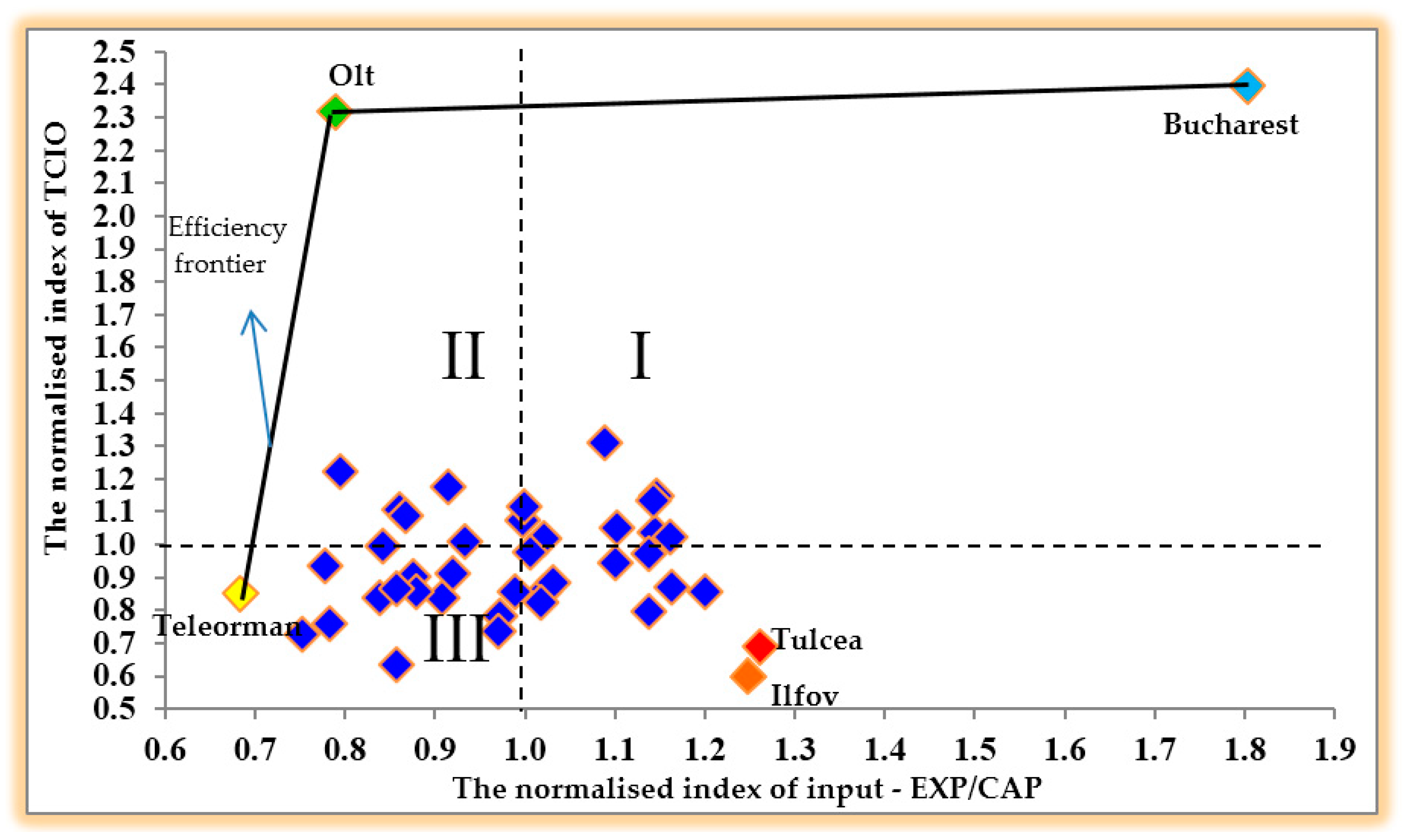
Finally, the global index of TCIO displays the highest values in Bucharest (2.39), followed by Olt (2.31), Cluj (1.31), Dolj (1.22), Prahova (1.17), Sibiu (1.15), Constanta (1.14), Suceava (1.12), Iasi (1.11) and six other counties with above-par values. The lowest values for the same measure can be found in Ilfov (0.60), Giurgiu (0.63) and Tulcea counties (0.69). Most of these statistical results, prior to the actual DEA analysis, were expected. On the one hand, the capital city Bucharest (which is assimilated to a county or even a region from the financial and demographic points of view) has the highest deviation indices for most measures as compared to the national average index, especially with the composite TCIO. More likely, this hypothesis will send the capital on the DEA efficiency frontier. On the other hand, we have also estimated (to obtain) general low values for the counties that are less populated and with a small surface area, such as Ilfov, Tulcea and Giurgiu.
Figure 2 reveals the distribution of counties according to their standardized input value and
TCIO output variable.
The figure displays counties’ inclusion in the space bounded by the frontier passing nearby the extremities’ points and represented by three counties, respectively Teleorman, Olt and Bucharest. Teleorman county is represented by the pair of coordinates (0.6839; 0.8489). This county records the lowest index of per inhabitant expenditures, represented graphically by its close positioning to the Oy axis, the axis of TCIO variable. Also located on the frontier efficiency curve is Olt, a county that succeeds to register close to maximum results, even with a relatively low level of input expenditures. The county’s coordinates are (0.7895; 2.3124), and it is located in the best quadrant, respectively far from the Ox axis (sustainable output) and close to the Oy axis (low inputs). Although the two counties are part of different regions (Teleorman county belongs to the South Muntenia Region, while Olt is part of the South-West Oltenia Region), they are situated close to each other, on the southern border, along the Danube River (see
Figure 1). Identifying Teleorman and Olt with maximum efficiency is unusual, and it was not expected. They are not characterized as rich or economically developed counties. None of their towns and municipalities have an airport; they lack foreign direct investments; have pretty high unemployment rates; and the proportion of their rural population is over 56%.
However, as we expected, Bucharest is placed on the efficiency curve, with coordinates of (1.8029; 2.3922). This proves this municipality’s LPAs use high financial resources, yet with good results in terms of public services provided to its inhabitants.
The cloud is made of 39 counties, and their inefficiency degree is measured by their distance to the frontier curve. The worst results were registered by the counties located far right and way down, i.e., the counties that spend more money (far from the Oy axis) and generate unsustainable outputs (are closer to the Ox axis) as compared to the rest of the counties. The counties of Ilfov (1.2496; 0.5954) and Tulcea (1.2624; 0.6885) may be included in the unsustainable and inefficient output typology.
In
Table 3, we present the input-oriented, respectively output-oriented, efficiency scores, for both
6 outputs/1 input and
1 output/1 input variants. Efficiency scores obtained for the two cases show that the average inefficiency level for the 42 counties increases as the number of output (as well as input, in general) variables decreases. As such, for input variables efficiency’s analysis, from an average score of approximately 0.88 in the case of aggregating the six output variables, we reach averages of around 0.73 for the
1 input/1 output model. For the output sustainability, starting from an average of 0.96 in the six measures scenario, we reach a quite low level of 0.45 in the
1 input/
1 output scenario.
4. Discussions
In this section and the following, we discuss the results and the way they can be interpreted in light of previous studies and working hypotheses. We continue discussing the findings and their implications in a broader context and highlight future research directions.
For the 1 input/1 output scenario, we can appreciate that, on average, the same level of results could have been generated using roughly 27% less resources. As a consequence, LPA performances at the counties, municipalities, towns and communes’ levels could increase without necessarily increasing the expenditures. A similar conclusion is available for the 1 input/6 outputs model, respectively the same level of local public services could have been obtained with about 12% fewer input resources.
When analyzing TCIO, the results show that output could have been at least 55% higher considering the input level. In 39 out of 42 counties, a higher or lower unsustainable use of public financial resources as a result in terms of the quantity and quality of local services provided to citizens does not reach residents’ expectations.
In the multiple outputs scenario, the average technical efficiency score is even higher than the input-oriented technical efficiency score. As such, for the 1 input/6 outputs case, the average score is almost 0.96, meaning the output level could have increased by about 4%.
Of the 42 decision units, 11 counties register a 100% efficiency level in the case of six output variables, and only three counties remain efficient in the 1 input/1 output case. Maximum efficiency counties are Teleorman, Olt and Bucharest.
After examining the two cases regarding the number of output variables and the efficiency scores for each county, the following patterns emerged:
Counties with higher local public expenditures per capita compared to the µ + σ/2 limit tend to have, in analyzing the efficiency of both input and output variables, lower efficiency scores compared to counties whose expenditures per inhabitant are below the aforementioned limit; the µ value represents the simple arithmetic average of per capita expenditures, whereas σ represents the standard deviation of each county’s expenditures per capita compared to the average;
Counties with local public expenditures per inhabitant higher than the µ + σ/2 limit tend to have lower efficiency scores for both input and output variables’ efficiency analysis, compared to counties whose expenditures per inhabitant are lower than the limit mentioned;
Counties with a higher number of population (above the 479,087 inhabitants average) registered better efficiency scores, usually above the average.
Table 4 presents average efficiency scores obtained grouping counties according to their level of local public expenditures per capita and the number of inhabitants.
For the two alternatives, efficiency scores tend to grow nearer the value of one, as the volume of public expenditures decreases. This is a natural situation considering that public expenditures per inhabitant are used as an input variable, measuring the efforts of the LPAs to service collective needs. As a consequence, we found that a level of expenditures of over 2280.49 Lei/inhabitant (µ + σ/2) leads to a lower efficiency. Average scores of counties with such expenditures for the two cases, 1 input/6 outputs and 1 input/1 output, are of 0.8049/0.9494, respectively 0.6278/0.4424, values situated below national averages of 0.8789/0.9594, respectively 0.7313/0.4474. The order of values is presented as input/output.
The only decision unit with 100% efficiency is Bucharest. Moreover, above average values were registered in the counties of Salaj (only for the output-oriented analysis), Brasov, Sibiu, Constanta (for the output and the 1 input/1 output variants), Valcea (for the output and the 1 input/6 outputs variants) and Timis (1 input/6 outputs for input efficiency analysis and in both cases for output efficiency analysis). Those results confirm the restrictive nature of the 1 input/1 output aggregate model.
The general average of input-oriented efficiency scores of counties with local budget expenditures below the 2280.49 Lei/inhabitant level (over and even below the other reference level of 1878.59 Lei/inhabitant) is of 0.9121 (1 input/6 outputs) and 0.7778 (1 input/1 output). For the output-oriented analysis, the average value of counties with expenditures below the mentioned threshold is of 0.9638 (1 input/6 outputs) and 0.4497 (1 input/1 output).
These results above are the aggregated efficiency average of all counties pertaining to each scenario. Using each county’s stable population in the analysis led us to conclude that there is a relative influence of the total number of persons upon efficiency scores. As such, counties with an above average population register higher than general average efficiency scores for both inputs and outputs.
Yet, there are counties with a small number of inhabitants displaying relatively high efficiency scores in the input-oriented model. We can mention here Teleorman and Olt, as well as Buzau, Braila, Ialomita, Maramures and Calarasi counties, which register above average values no matter the output variables’ number. For the output-oriented model, the counties of Teleorman, Olt and Sibiu display above average values, regardless of the number of output variables, as well as Buzau, Salaj, Alba, Covasna, Harghita, Braila, Gorj, Valcea and Hunedoara.
As we stated in the Introduction section of this paper, the specific literature review is poor in similar studies. However, the analysis conducted in 2006 by Afonso and Fernandes [
14] represents an important reference for us. Although their study did not present any discussions on a possible relation between the technical efficiency score and the number of inhabitants of each Portuguese municipality, there are similarities between the two papers with respect to the connection between the per-capita expenditure level, the input itself and the degree of efficiency and sustainability of local public services provision. Similarly, municipalities with higher input level than the
μ +
σ/2 limit tend to have lower efficiency values than the ones with lower per-capita expenditures levels.
We have constructed a hierarchy according to the number of output variables and the way the scores are interpreted (by input or by output).
Seventeen out of the 36 counties displaying rank differences in the hierarchy based on input and output efficiency have higher efficiency scores for the input variable, minimizing expenditures to generate the same output, whereas 20 counties register higher efficiency scores for output variables, looking to optimize their level using available resources.
According to the results obtained, the counties can be grouped as such:
Counties registering better scores for input-oriented analysis are Maramures, Satu-Mare, Covasna, Bacau, Botosani, Iasi, Vaslui, Braila, Buzau, Galati, Vrancea, Calarasi, Dambovita, Giurgiu, Ialomita, Ilfov and Gorj;
Counties registering better scores for output-oriented analysis are Bihor, Bistrita Nasaud, Cluj, Salaj, Alba, Brasov, Harghita, Mures, Sibiu, Neamt, Suceava, Constanta, Tulcea, Prahova, Mehedinti, Valcea, Arad, Caras-Severin, Hunedoara and Timis;
Counties with same ranking for both input- and output-oriented analysis are Arges, Teleorman, Bucharest, Dolj and Olt.
We find that counties with better results for both input-oriented efficiency, as well as ones with good results for output-oriented efficiency do not have an above par average index for all output variables. The first group has an average output index of 0.8452, for a level of 1867.33 Lei average expenditures per capita or 11.36% below overall average of 2079.54 Lei/inhabitant.
The second group, for a 2311.45 Lei level of expenditures per capita, or 11.15% above the average, has registered an average output index of 0.9885.
The third group, i.e., the counties constant in ranking both in input and output terms, registered an above par average output index of 1.5725, for a 2054.58 lei average level of expenditures per capita (the arithmetic average for these five counties), situated 1.2% below the average level for 42 entities.
The hierarchy established according to the results obtained applying the two variants proves certain counties occupy very different positions. For example, Cluj county takes 30-th place in 1 input/1 output analysis and first place in 1 input/6 outputs analysis.
Counties such as Giurgiu, Dambovita, Calarasi, Vrancea and Maramures loose between six and 29 positions in the analysis of local public services’ efficiency, as compared to their expenditures’ efficiency analysis. Significantly better results in analyzing output-oriented efficiency as compared to the input-oriented one are recorded in Bihor, Bistrita Nasaud, Arad, Timis and Hunedoara. They gain between three and 22 positions in the rankings for the two analyzed variants.
Afonso and Fernandes have also obtained some interesting variations in individual ranking positions considering first input and then output efficiency results. They obtained a decrease of the relative ranking positions of non-metropolitan municipalities, of more than ten places when measuring output efficiency compared to input efficiency results and an improvement of other municipalities relative ranking when considering output efficiency rather than input efficiency.
Similar to our paper, the two above-mentioned groups of observations are characterized by one distinguishing feature. On the one hand, the administrative-territorial units that perform better in terms of input efficiency, despite registering average levels of per-capita expenditures below the overall average sample, report a total performance indicator below the average sample. On the other hand, the municipalities that perform better in terms of output efficiency, despite having on average levels of per-capita expenditure above the overall sample average, report a total output indicator superior to the overall average sample.
Alternative results, with a higher number of counties identified by default as efficient and with a higher output efficiency score, could have been recorded if our input variable was the total expenditure value of each county, without dividing it to the total number of inhabitants. Still, the approach we had by using the ‘per-capita size dimension’ captures much better the uncontrollable demand-based dynamics of local services provision.
5. Conclusions
We have researched local public expenditures’ efficiency for the 42 Romanian decision units using the DEA model. We have selected variables as one input (local public expenditures per capita) and six outputs (standardized values of local public services of general services, basic education, social services, water supply system, culture and recreation and public utilities).
We have continued analysis using one input variable and one output variable, called TCIO, based on a simple arithmetic average of six initial standardized variables. According to the research objectives, we have conducted analysis as input-oriented (minimizing input whilst achieving the same output level) and output-oriented (maximizing output with a given amount of input).
As a conclusion, the input and output efficiency scores suggest that, on average, Romanian counties are relatively inefficient. The results show only three decision units, Teleorman, Olt and Bucharest, have registered maximum efficiency levels. Considering average efficiency scores obtained for input and output-oriented analyses, we can appreciate that overall, counties could have generated the same level of local services using 26.87% less resources. This means increasing expenditures does not guarantee LPAs’ increased performance levels. At the same time, counties would have achieved better use of funds available for providing local public services if they had produced an extra 55.26% more community services; or, given the existing amount of available resources, they should have provided more services and goods for their citizens. Consequently, we may state that, in Romania, local development analyzed through the relationship between the financial resources used and the quantity and quality of the services offered at the county level is not yet fully configured to generate sustainability.
However, using more variables in our model, the average efficiency score increases along with the number of decision units located on the efficiency frontier. Moreover, our study proved the existence of a significant dispersion of different counties’ performances. Usually, counties with lower expenditures per capita obtained above average efficiency scores. This finding seems to confirm the general opinion that increased public spending does not necessarily imply better services for the citizens. In other words, local performance and the degree of sustainability of local public services delivery could be improved without necessarily increasing county or municipal spending.
The identification of 11 efficient units, instead of three, in the case of using more outputs, is a trade-off to avoid losing relevant information. This does not seem to be critical in our case. We do not consider that an alternative analysis with more inputs and outputs should be developed.
As an argument for the last statement, by all output measures selected for DEA analysis, we took into consideration all major locally-provided functions of an LPA. The focus is on global county performance stemming from the provision of specific services (e.g., general public services, education, social care, basic public utilities, culture and recreation, local interest public utility). With respect to the existence of a single input variable, selecting total per-capita county expenditure guarantees at least that all inputs are considered in the analysis. This variable is a more realistic county input measure if one acknowledges the reduced county authorities’ room for influencing different expenditure choices, especially current expenditures. Similar approaches are found in the works of Afonso and Fernandes (2006), as well as of Fisher’s (2007), De Borger and Kerstens’ (2000), Deller and Rudnicki’s (1992) [
40,
41,
42]. Deller and Rudnicki proxy the input of selected output ‘administrative services’ with the ‘school expenditures on administration per pupil’ variable in their work on Maine’s public education services and, as such, use only the
1 input/
1 output scenario.
In addition, one important issue regarding our panel of data is that both input and output indicators are subject to data availability constraints. Assuming we introduce more inputs and/or outputs within DEA linear processing of data, we might have not complied with the rules described in Subsection 2.2 regarding the connection between the number of input and output variables and the total number of observations.
Afonso and Fernandes (2006) also identified the pattern we have mentioned before, i.e., the higher per-capita expenditure level, the lower efficiency scores. Considering both individual efficiency scores and ranking positions of the units described in each research paper, we reached a similar conclusions, respectively our results reveal a wide dispersion in performance and sustainability.
Another conclusion of our analysis which, in this case, was not to be found in other DEA research papers relates to the number of inhabitants. An increased number of inhabitants (and implicitly of taxpayers) contributed to increased efficiency scores (closer to par value). Between two counties having similar expenditures, the one with a higher number of inhabitants will show lower expenditures per capita, thereby corresponding to the aforementioned typology.
Many studies suggest technical efficiency varies systematically with the socio-economic, as well as environmental characteristics of the counties. These results are confirmed by Deller and Rudnicki (1992) and Cooper and Cohn (1997), who analyze schools’ technical efficiency (along with its determinants) in the U.S. states of Maine and South Carolina [
42,
43].
As pinpointed in the first sections of the article, Romania faces some general problems of economic development and budgetary imbalances. The significant local budget deficits are covered from the state budget or other governments, via transfers, such as subsidies, income tax and VAT. These are absolutely necessary especially for those counties and regions suffering severe financial shortages.
These are absolutely necessary especially for those counties and regions suffering severe financial shortages.
At least from a theoretical point of view, increasing attention has been given for a few decades now to the efficiency and sustainability of public expenditures and public services in European countries (e.g., European Commission, 2004), as well as at the international level. People became aware of how important and necessary access to the best public social and educational services is. The variety of public services is essential for the poor and the rich, for men and women, for young and elderly people, for urban and rural communities, for consumers with a lower or a higher level of education.
We aim that the results of our work will be useful to researchers, professionals and the general public interested in understanding the inner mechanisms of efficient and sustainable local public services. The authors of this study have intended for this research to be conducive in motivating people and politicians from less efficient counties to demand better performance and improvement of public goods and services. Further analysis should be conducted especially for territorial-administrative units of developing countries, where disparities across regions, districts and municipalities are more evident. For future studies, we suggest introducing other input and output variables, according to available data, using measures for cross-country comparisons or even comparisons for different periods of time between one country’s chosen local levels.


