Article

A Hybrid Multi-Step Rolling Forecasting Model Based on SSA and Simulated Annealing—Adaptive Particle Swarm Optimization for Wind Speed

1
School of Statistics, Dongbei University of Finance and Economics, Dalian 116025, China
2
Key Laboratory of Arid Climatic Change and Reducing Disaster of Gansu Province, College of Atmospheric Sciences, Lanzhou University, Lanzhou 730000, China
*
Author to whom correspondence should be addressed.
Sustainability 2016, 8(8), 754; https://doi.org/10.3390/su8080754
Submission received: 22 May 2016 / Revised: 15 July 2016 / Accepted: 27 July 2016 / Published: 6 August 2016

Abstract

:
With the limitations of conventional energy becoming increasing distinct, wind energy is emerging as a promising renewable energy source that plays a critical role in the modern electric and economic fields. However, how to select optimization algorithms to forecast wind speed series and improve prediction performance is still a highly challenging problem. Traditional single algorithms are widely utilized to select and optimize parameters of neural network algorithms, but these algorithms usually ignore the significance of parameter optimization, precise searching, and the application of accurate data, which results in poor forecasting performance. With the aim of overcoming the weaknesses of individual algorithms, a novel hybrid algorithm was created, which can not only easily obtain the real and effective wind speed series by using singular spectrum analysis, but also possesses stronger adaptive search and optimization capabilities than the other algorithms: it is faster, has fewer parameters, and is less expensive. For the purpose of estimating the forecasting ability of the proposed combined model, 10-min wind speed series from three wind farms in Shandong Province, eastern China, are employed as a case study. The experimental results were considerably more accurately predicted by the presented algorithm than the comparison algorithms.

1. Introduction

Energy plays a vital part in modern social and economic development. Along with the rapid development of technology in the last few decades, energy demands continue to increase rapidly [1]. In accordance with the IEA World Energy Outlook 2010, China and India will be responsible for approximately 50% of the growth in global energy demand by 2050. The consumption of energy in China will be close to 70% greater than the energy consumed by the United States today. Second only to America, China will become the second leading energy-consuming country in the world. Nevertheless, China’s per capita energy consumption will remain lower than 50% of that of the USA [2]. Since conventional energy sources such as coal, natural gas, and oil for electricity generation are being quickly depleted, sufficient energy reserves and sustainable energy problems are garnering increased attention. Additionally, using traditional resources produces large amounts of carbon dioxide, which may lead to global warming, and is considered an international security threat. Therefore, it not only affects the environment, it also threatens the safety of individuals and the planet [3].
Consequently, to alleviate the pressure of this energy shortage, renewable energy sources are being explored and the sustainable development of green energy has become a significant measure of global energy development success [4]. Obviously, it has become necessary to seek and develop new environmentally friendly sources of renewable energy. Wind energy, the most significant new type of green renewable energy [5], is steady, abundantly available, reliable, inexhaustible, widespread, pollution-free, and economical. It contains enormous power and its usage does not harm the environment by creating greenhouse gas emissions. Furthermore, it has been considered or applied in the production and development for energy in a host of countries. In modern times, wind energy has become the most indispensable and vital renewable energy source globally. The fast growth of the power system enables the absorption of large amounts of wind power. However, in consideration of stochastic factors such as temperature, atmospheric pressure, elevation, and terrain, it is still difficult to make an accurate forecast, which can also give rise to trouble in terms of the energy transmission and the balance of the power grid. Hence, developing an effective approach to overcome these challenges is necessary.
In order to reduce time series prediction errors, thousands of methods have already been studied. First, many effective data denoising tools, including the Wavelet Transform (WT), the Empirical Mode Decomposition (EMD) [6,7,8], the Wavelet Packet Transform (WPT), the Singular Spectrum Analysis (SSA) [9], and the Fast Ensemble Empirical Mode Decomposition (FEEMD) algorithm [10], have been applied to process the original data to achieve a relatively higher forecasting accuracy. For instance, SSA, as a novel analytical method, is especially suitable for research into periodic oscillation, which has proven to be an effective tool for time series analysis in diverse applications; the results indicate that it can effectively remove the noise of the wind speed data to improve forecasting performance. Secondly, different prediction approaches are applied to time series forecasting, including SVM, ARMA, ANNS, etc. According to various researchers, these methods can be categorized into four classes [11]: (i) purely physical arithmetic [12,13,14]; (ii) mathematical and statistical arithmetic [15,16,17,18,19,20,21]; (iii) spatial correlation arithmetic; and (iv) artificial intelligence arithmetic [22].
Purely physical arithmetic not only utilizes physical data such as temperature, density, speed, and topography information, but also physical methods, including observation, experiment, analogy, and analysis, to forecast the future wind speed. However, these approaches do not possess unique advantages for short-term prediction. Mathematical and statistical methods, such as the famous stochastic time series models, typically make use of historical data to forecast the wind speed, which can be easy to employ and simple to realize. Therefore, some categories of time series models are often used in wind speed forecasting. Some examples that can be utilized to obtain excellent results include the exponential smoothing model, the autoregressive moving average (ARMA) model [18], filtering methods, and the autoregressive integrated moving average (ARIMA) model [23,24]. Distinct from other methods, spatial correlation arithmetic may achieve better prediction performance. Nevertheless, it is extremely difficult to obtain a perfect application due to the abundant amount of information that must be considered and collected. In recent years, as artificial intelligence technology has developed and become widely used, many researchers have utilized intelligence algorithms in their papers, including artificial neural networks (ANNs) [25,26,27,28,29], Support Vector Machine (SVM) [30,31], and fuzzy logic (FL) methods [32,33], which can be applied to combine new algorithms for enhancing wind speed forecasting ability.
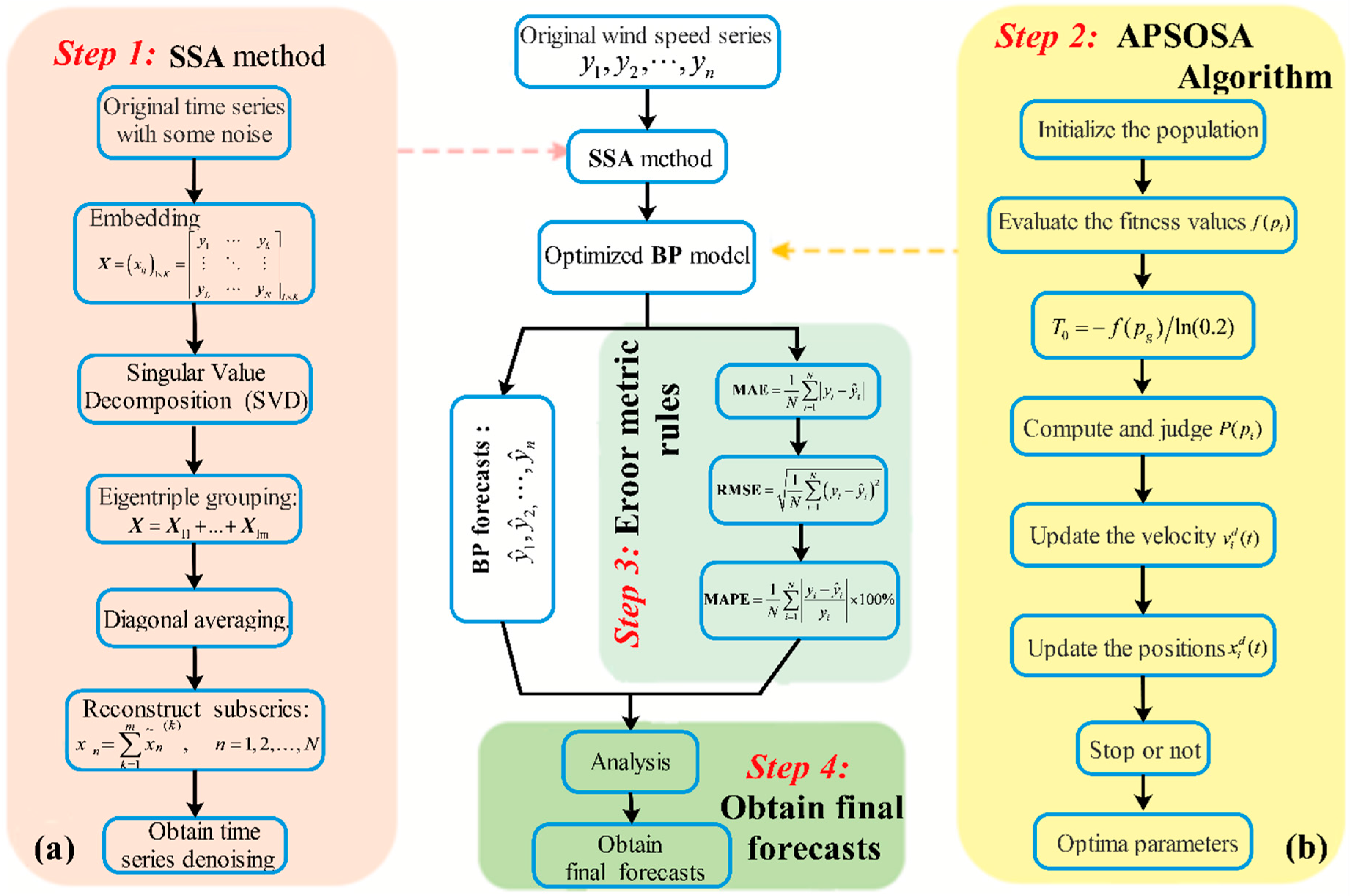
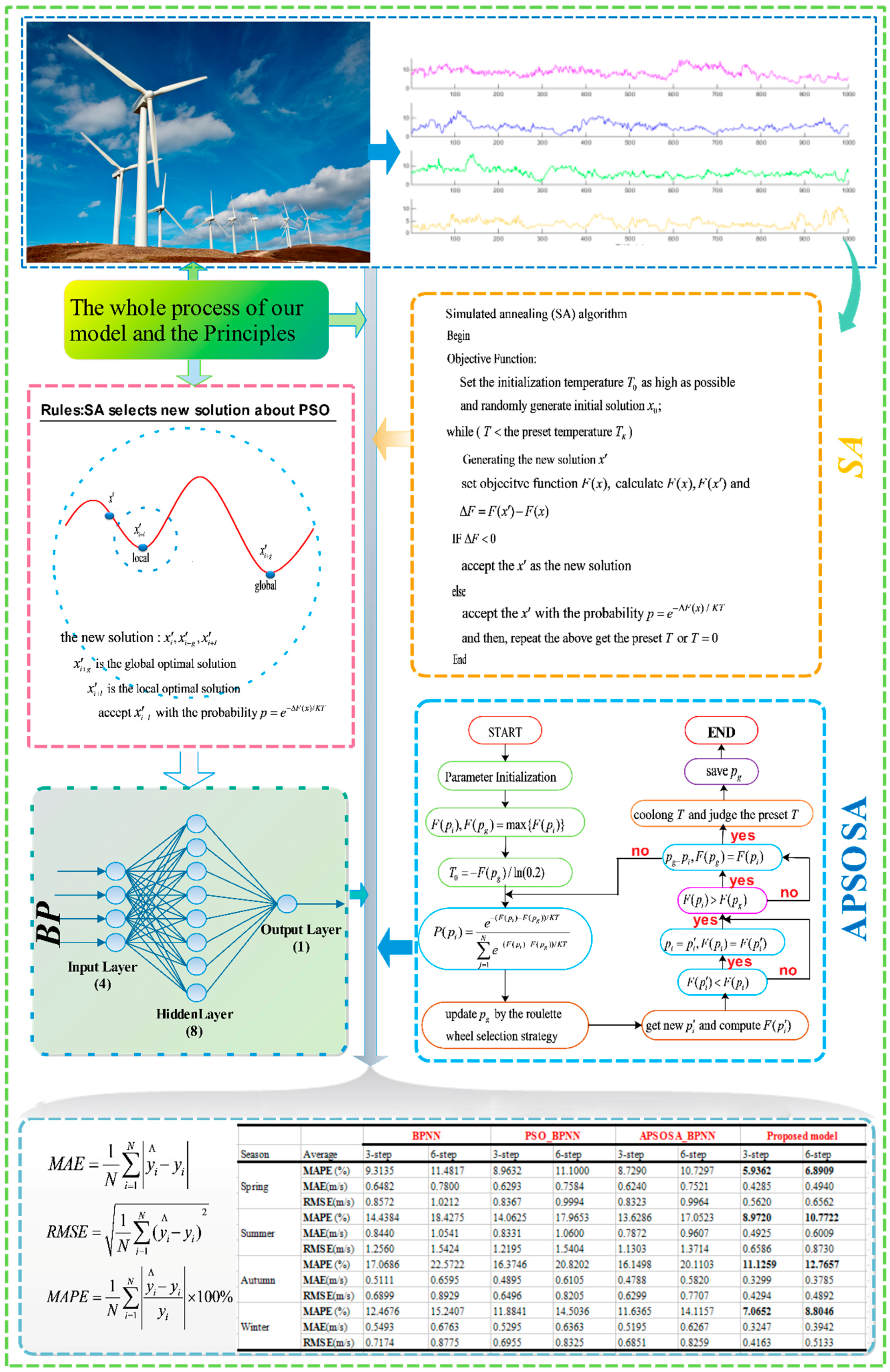
In this research, a hybrid algorithm was proposed with the goal of achieving better forecasting performance. Firstly, in comparison with other methods, including WNN (Wavelet Neural Network) and GRNN (generalized regression neural network), BPNN provides the best prediction performance for both half-hour and one-hour time frames. Therefore, BPNN was selected for use in our models. Next, as a different analytical method, SSA is employed to construct, decompose, and reconstruct the trajectory matrix. SSA can extract different components of the original signal, such as the long-term trend of the signal, a periodic signal, and noise signals, and is capable of removing the noise from the original signal. Next, the optimization algorithm APSOSA, combining APSO [34,35,36,37,38] and SA [39,40,41,42], can enhance the prediction accuracy and convergence of the basic PSO algorithm. Moreover, APSOSA is able to avoid falling into local extreme points so that the parameters of the Back Propagation neural network (BPNN) can be better optimized. Finally, to achieve better forecasting performances, the wind speed data after noise elimination are input into the BPNN. In addition, four commonly used error criteria (AE, MAE, MAPE, and MSE) are applied to assess the performance of the raised hybrid algorithm. The main aspects of the model are introduced as follows: (1) data preprocessing; (2) the best forecasting method, BPNN, is selected and its parameters are tuned by an artificial intelligence (APSOSA) model; (3) forecasting; and (4) comparison and analysis.
The main contributions of this paper are summarized as follows:
(1)
With the aim of reducing the randomness and instability of wind speed, the Singular Spectrum Analysis technique is applied to decompose the wind series data, revealing real and useful signals from the wind series.
(2)
The best prediction system, BPNN, is selected from the different methods, including WNN, GRNN, and BPNN.
(3)
In view of the shortcomings of the PSO algorithm, APSOSA is developed to optimize parameters, which can assist the individual PSO in jumping out of the local optimum. Ultimately, parameters are selected and optimized by combining their respective advantages.
(4)
To examine the stability and accuracy of the new combined forecasting algorithm, 10-min wind speed series from three different stations are used in the experimental simulations. The experimental results indicate that the novel hybrid algorithm has a higher performance, significantly outperforming the other forecasting algorithms.
(5)
Giving full consideration to the other influential factors in the experiments, such as the seasonal factors, the geographical factors, etc., according to the results, this action proves that the new combined algorithm has a powerful adaptive capacity, which can be widely applied to the prediction field.
(6)
The Bias-Variance Framework and statistical hypothesis testing are employed to further illustrate the stability and performance of the proposed algorithm.
The remainder of this paper is designed as follows. The methodology is described specifically in Section 2. To verify the prediction accuracy of the raised algorithm, a case study is examined in Section 3. Next, the wind farms area and datasets are introduced in Section 3.1, whereas Section 3.2 displays the performance criteria of the forecast results. In Section 3.3, the results of the different algorithms are listed and compared with the proposed algorithm. In order to further illustrate the stability and performance of the proposed algorithm, in Section 4, the Bias-Variance Framework and statistical hypothesis testing are employed. Finally, the conclusions are provided in Section 5.

2. Methodology

In this section, all of the algorithms involved in this work are described. The full list of algorithms to be discussed in this section is as follows: the singular spectrum analysis algorithm, an efficient technology for time series analysis; the particle swarm optimization algorithm; the simulated annealing algorithm, which overcomes PSO falling into the local minima, and the back propagation neural network. The hybrid algorithm-APSOSA, raised to search for the optimal parameters of BPNN, will also be introduced in detail.

2.1. Singular Spectrum Analysis

Compared with other nonparametric approaches, such as EMD, which exhibits a potential mode-mixing problem, and EEMD, which does not completely neutralize the added white noise, singular spectrum analysis (SSA), which overcomes the traditional analysis methods’ (such as Fourier analysis) shortcomings, has been proven to be one of the most effective and powerful methods in time series analysis. It was developed by Broomhead and King in 1986 [43]. Figure 1 shows the decomposed series of wind speed by SSA. The details are shown in Appendix A.1.

2.2. Intelligent Optimization Algorithms

In this section, several optimization algorithms will be introduced.

2.2.1. Particle Swarm Optimization

Inspired by imitating the social behavior of flocks of bird and schools of fish, an effective approach for optimization, Particle swarm optimization (PSO), was first developed by Dr. Eberharts and Dr. Kennedy in 1995 [44]. It is a stochastic, population-based evolutionary algorithm, which involves searching for solutions [39] (details in Appendix B.1).

2.2.2. Back Propagation Neural Network

First proposed by Rumelhart and McCelland (1986) [45], the Back Propagation Neural Network (BPNN) is one of the most widely employed artificial neural network (ANN) models (details in Appendix B.2). It is not only capable of learning and storing a large amount of input–output mode mappings without needing to reveal the mathematical equations of the mapping relationship, but can also apply the steepest descent method, by back propagation, to constantly adjust the network weights and thresholds, resulting in the minimum square error. In addition, BPNN [46] consists of three layers: the input layer, the hidden layer, and the output layer. The experimental parameters are listed in Table 1.

2.2.3. Simulated Annealing

The concept of Simulated Annealing was first introduced by N. Metropolis et al. in 1953. In 1983, Kirkpatrick et al. succeeded in introducing SA in the field of combinatorial optimization [47]. Based on the Monte-Carlo iteration solving method, currently the SA algorithm has become one of the most popular heuristic random search methods. Unlike the PSO algorithm, SA can jump out of the trap of local minima in a timely manner to update the solutions and obtain the global optimum (details in Appendix B.3).

2.2.4. The Proposed Optimization Algorithm, APSOSA

This paper proposes a hybrid APSO algorithm by employing the SA algorithm to prevent the PSO from falling into local minima (the algorithm of SA-APSO is shown in Table 2). The major steps of the hybrid optimization algorithm are as follows. First, enhance the accuracy and convergence rate of the basic PSO algorithm by applying a compression factor and selecting suitable parameters. Next, by combining the Simulated Annealing characteristics, PSO can more easily and quickly obtain the optimal solution in a larger search space. SA can also cancel the restrictions on speed border. Moreover, the Roulette Wheel Selection Strategy is chosen, shown in Figure 2, in this algorithm.
PSO can obtain better results in a faster setting with fewer parameters and is cheaper than other methods. It is also currently being widely used for promising results in continuous problems. However, the movement directionality of the particles is not certain, and particles are likely to jump out to obtain near-optimal solutions and their local search ability is relatively weak and easily trapped by the local optimum. Therefore, PSO is combined with the simulated annealing algorithm. The annealing algorithm is used when poor quality is probable to temporarily accept some solution features to construct a particle swarm algorithm, based on simulated annealing. A multitude of papers have verified that the improved particle swarm optimization algorithm obtains better results and have documented the effectiveness of the method through experimental simulation results. The velocity and position updating formula are as follows:
v i , j ( k + 1 ) = χ   [ v i , j ( k ) + c 1 r 1 ( p i , j ( k ) x i , j ( k ) ) + c 2 r 2 ( p g , j ( k ) x i , j ( k ) ) ]
x i , j ( k + 1 ) = x i , j ( k ) + v i , j ( k + 1 ) , j = 1 , ... , n
where r 1 and r 2 are set randomly between 0 and 1, and the learning factors c 1 and c 2 are positive numbers, where χ is computed by the following formula:
χ = 2 | 2 C C 2 4 C | ,    C = c 1 + c 2 ,   C > 4
In Equation (3), applying the best group positions, all particles fly to the best group positions, and then tend to the local minima solution if the best group positions are in the local minimum. Accordingly, this situation will cause the search dispersability and ability to become worse. To overcome this weakness, a new position p g will be selected from among the p i to replace p g . Finally, in this paper, the Equation (1) is rewritten as the following formula, Equation (4):
v i , j ( k + 1 ) = χ   [ v i , j ( k ) + c 1 r 1 ( p i , j ( k ) x i , j ( k ) ) + c 2 r 2 ( p i , j ( k ) x i , j ( k ) ) ]
However, how to address the suitable position p i is one of the most critical steps of the combined algorithm. Clearly, better performance of p i shall be considered a higher priority. Under the characteristics of the SA algorithm, the best solutions of every particle p i should be taken as the special one, which may be worse than the global optimal solution p g . Therefore, in the case of temperature T, we can calculate the leap probability using Equation (5):
P l p ( p i ) = e ( F ( p i ) F ( p g ) ) / K T
where F is the objective function value of the particle position.
The leap probability can be computed by the following formula, Equation (6):
P ( p i ) = e ( F ( p i ) F ( p g ) ) / K T   j   =   1 N e ( F ( p i ) F ( p g ) ) / K T
where N is the population, on the side; considering the Roulette Wheel Selection strategy, we can randomly choose the p i , which will be regarded as p g .
The chief steps of the APSOSA algorithm are as follows, and a flowchart is depicted in Figure 2.
  • Step 1: Set the initial temperature, and initialize the population along with every particle velocity and position.
  • Step 2: Compute F ( p i )   ( i = 1 , .. , N ) , where N is the updated population.
  • Step 3: Update the present position and fitness value of each particle by using p i , F ( p i ) and p g , F ( p g ) , respectively.
  • Step 4: Compute the initial temperature using Equation (7):
    T 0 = F ( p g ) / ln ( 0.2 )  
  • Step 5: Update the particle position and velocity and compute P ( p i ) .
  • Step 6: Through the roulette wheel selection strategy, the new global optimal solution p g is not regarded as p g until P ( p i ) > rand   (   ) .
  • Step 7: Update every particle velocity and position by the pre-set update formula.
  • Step 8: Compute every particle F ( p i ) , and then do not apply p i F ( p i ) to update the current global position p g and optimal fitness value F ( p g ) , respectively, until F ( p i ) > F ( p g ) .
  • Step 9: By applying the pre-set rules, the temperature reduces slowly.
  • Step 10: Analyze whether the pre-set conditions are met; if they have been met, output the information of p g and then end running. Otherwise, repeat the above steps, beginning with Step 5.

2.2.5. SSA–APSOSA–BPNN Algorithm

In this section, we will introduce the hybrid model (SSA–APSOSA–BPNN) more clearly. The flowchart of the model is described in Figure 3. And the experimental parameters of APSOSA are given in Table 3. The hybrid algorithm contains four main stages.
  • Stage I: Data prepossessing. Utilize the SSA method to process the original wind speed signals; as a result, the noise signals are removed, and the real and effective signals, which are shown in Figure 1, can be preserved. Lastly, the useful processed signal will be fed into the abovementioned hybrid model.
  • Stage II: Data selection. The processed valid data from Stage I is classified into three parts: the training set, the validation set, and the test set for model training, validation, and testing, respectively.
  • Stage III: Algorithm training and validation. Here, the SSA–APSOSA–BPNN algorithm is utilized for wind speed forecasting. Additionally, the detailed rules are given as below:
    • Step 1: Determine and initialize the parameters of APSOSA.
    • Step 2: Set the fitness function; the mean absolute error (MAE) of validation is taken as the fitness of the particles:
      f i t n e s s = M A E = 1 N i   =   1 N | y i y ^ i |
      where N is the number of validation sets and y ^ i and y i stand for the predictive value and the observed value, respectively.
    • Step 3: Update the historical extremum p j of every particle and the global extremum p g and then repeat the above rules for the next particles.
    • Step 4: Set the conditions and judge whether the fitness value meets the conditions; if it does, save the corresponding optimal parameters and then stop running. Otherwise, run Step 3 again and continue to run.
  • Stage IV: Forecasting. In this stage, the optimal parameters from Step 4 of Stage III will be applied into the BPNN model to forecast. Finally, the wind speed forecasting data will be obtained by completing all of the above steps.

3. Case Study

To examine the accuracy of the novel combined algorithm, four different multi-step forecasting algorithms are compared by analyzing the three-step-ahead-prediction (half–1-h-ahead) and the six-step-ahead-prediction (1-h-ahead) of a 10-min wind speed series at three different wind power stations.

3.1. Study Area and Datasets

Shandong, located on the east coast of China, is not only one of the provinces with the largest economy, but also one of the biggest energy consumers. However, 99% of the electrical energy comes from coal power generation. As a result, Shandong faces enormous energy pressures.
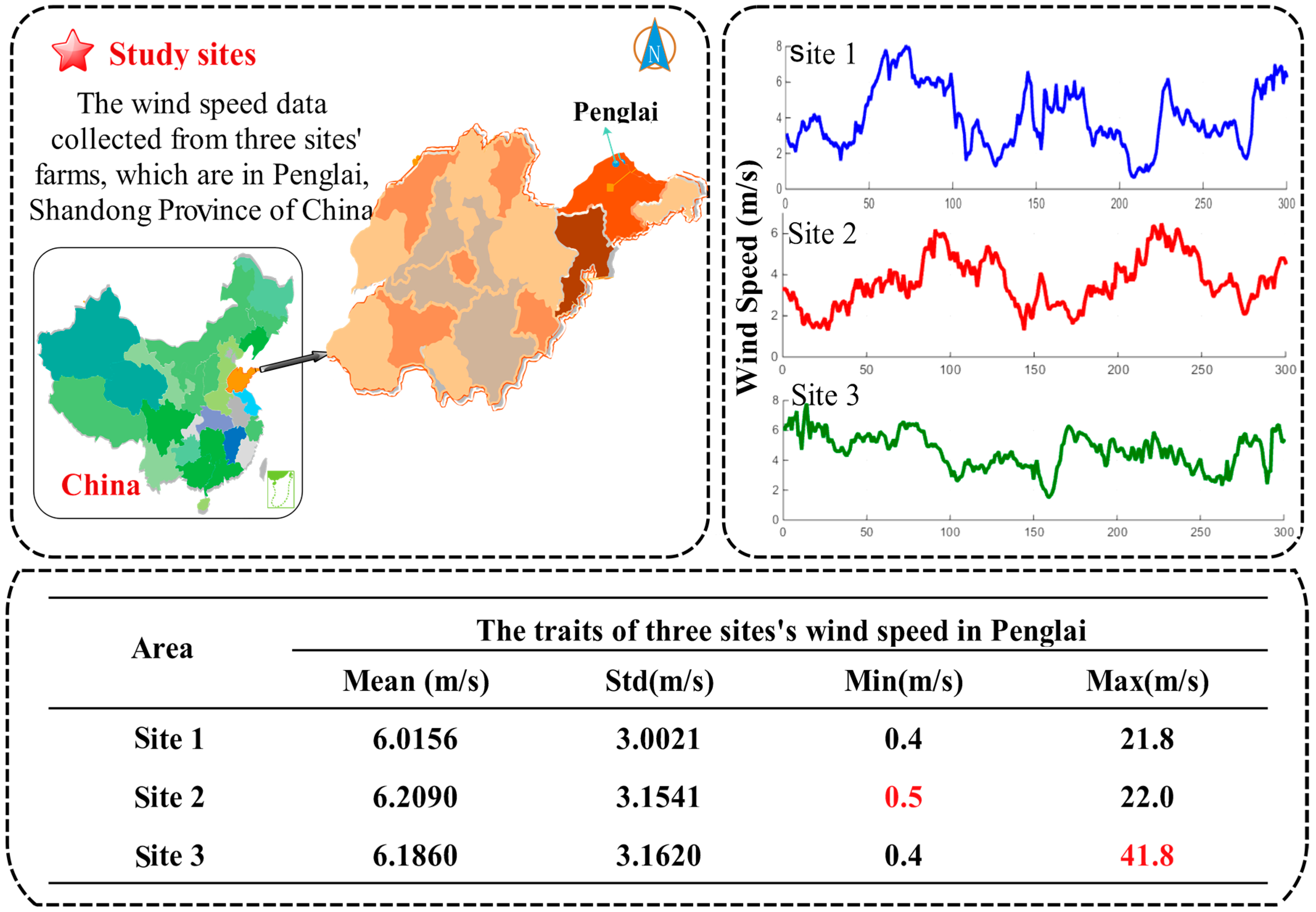
However, as a coastal province, Shandong possesses one of China’s largest wind farms, with an installed capacity of 58 million kilowatts. A simple map of the research area is depicted in Figure 4. With the aim of satisfying social development, achieving energy conservation, and protecting the environment, Shandong has begun developing wind power stations. Due to the area’s unique geographical advantages, capacity reached 260 billion KWH in 2007. In addition, the Shandong Province Bureau of Meteorology assessment notes that the entire output of wind energy resources in Shandong province is 67 million kilowatts, which is equivalent to the installed capacity of 3.68 times the capacity of the Three Gorges Hydro-power Station (18.20 million kilowatts), which ranks in the top three. To actively build wind power green energy bases, promote wind energy development, and protect the environment, Shandong has been focusing on building large-scale wind farms in Weihai, Yantai, Dongying, Weifang, Qingdao, and other coastal areas, and is gradually developing offshore wind power projects.
In this work, Penglai, which is located north of Shandong and lies north of the Yellow Sea and the Bohai Sea, was chosen as the area of study. It has tremendous, potentially valuable wind resources. The specific advantages are as follows: (i) higher elevation but relatively flat hilltops, ridges, and a special terrain that has much potential as an air strip; (ii) longer cycle of efficient power generation; (iii) suitable climatic conditions that are conducive to the normal operation of wind turbines; and (iv) small diurnal and seasonal variations of wind speed, which can reduce the impact on power.
In this study, the 10-min wind speed data from Penglai wind farms are used to obtain a detailed example for evaluating the performance of the proposed model. First, the wind speed data are divided into four parts according to the seasons, so that the impact of seasonal variations can be considered to increase the stability of the proposed model. Next, every seasonal wind speed dataset is divided into three parts: a training set, a validation set, and a testing set. Additionally, the noise is removed from the data by using SSA. Finally, the processed data are entered into the model and, judging from the forecasting results, we determine whether the raised algorithm can be widely employed for real-world farm use. In this study, the experiment is applied to three different sites (Site 1, 2, and 3). The above-described experiment is scientific and is used to validate the performance of the proposed model.

3.2. Performance Criteria of Forecast Accuracy

To evaluate the prediction accuracy of the raised hybrid algorithm, four indexes are applied to measure the quality of the forecasting methods: absolute error (AE), mean absolute error (MAE), root mean square error (RMSE), and mean absolute percent error (MAPE), shown in Table 4 (here N is the number of test samples, and y ^ i and y i represent the real and forecast values, respectively). Here, the absolute error (AE) and the mean absolute error (MAE) are both selected so that the level of error can be more clearly reflected. RMSE is chosen because it can easily reflect the degree of changes between the actual and forecasted value. Additionally, MAPE is chosen because of its ability to reveal the credibility of the forecasting model. Wind speed forecasting errors are related to not only the forecasting models but the selected samples. Consequently, the forecasting errors within a certain scientific range can be accepted. Moreover, in order to better evaluate performance, four percentage error criterions are also applied in this study, listed in Table 5.

3.3. Experimental Simulations

In this subsection, three single models, WNN, GRNN, and BPNN, are compared to obtain the best prediction approach. As a result, whether for half-hour (rolling three-step) or one-hour (rolling six-step) predictions, BPNN gives the best prediction accuracy (see Table 6 and Table 7) of the four proposed models. Next, the APSOSA-BPNN is selected from BPNN, PSO-BPNN as the best prediction algorithm. Finally, the hybrid SSA–APSOSA–BP algorithm was proposed as our best prediction model.
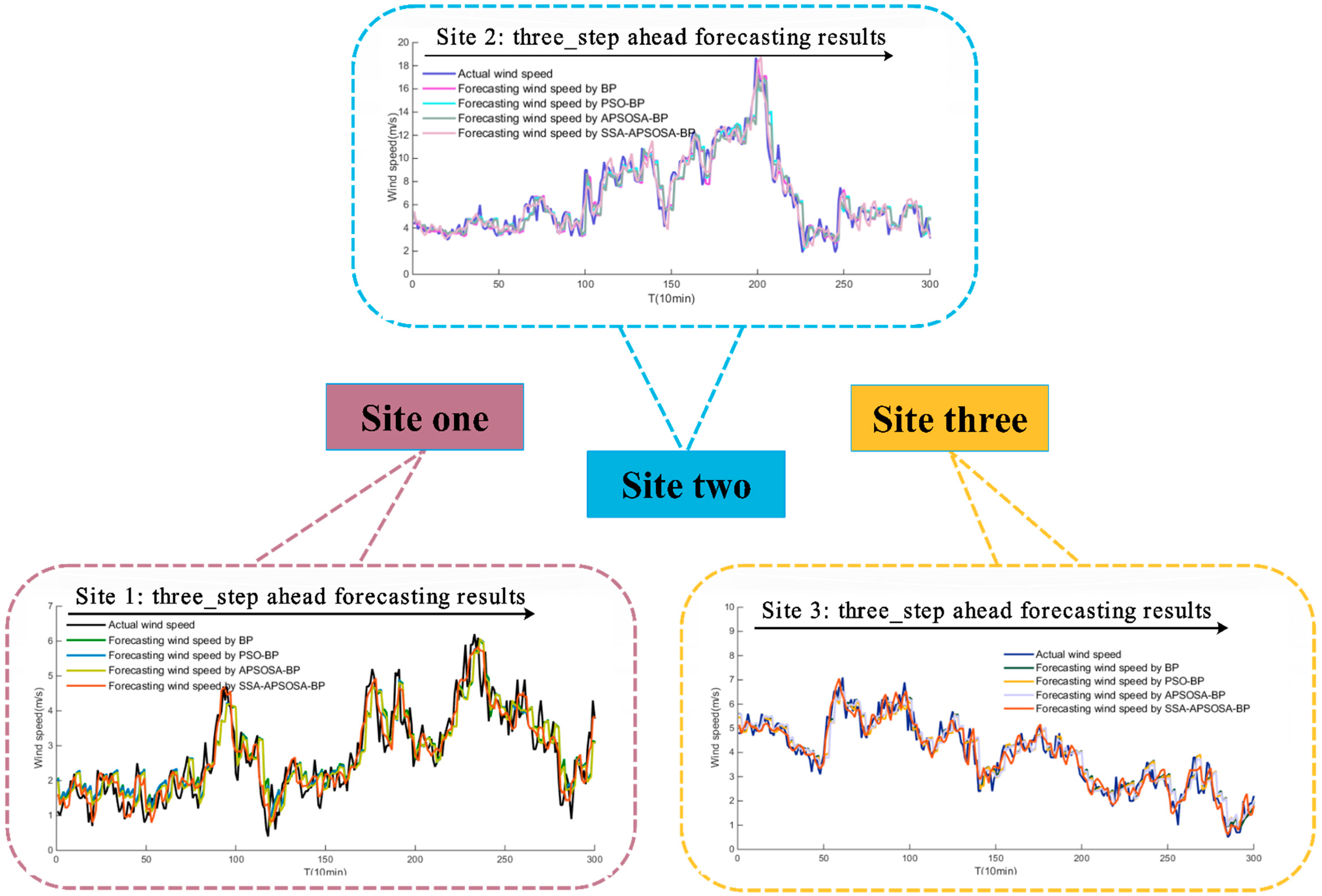
The BPNN, PSO-BPNN, and APSOSA–BPNN hybrid algorithms were selected to compare the forecasting results. Three sites from the Shandong–Penglai wind farms were selected, and then a sample (the 10-min wind speed series) of every season from each site was selected and entered into the above algorithms. Next, the multi-step predicted results were displayed. The specific results of the three sites are shown in Table 6 and 
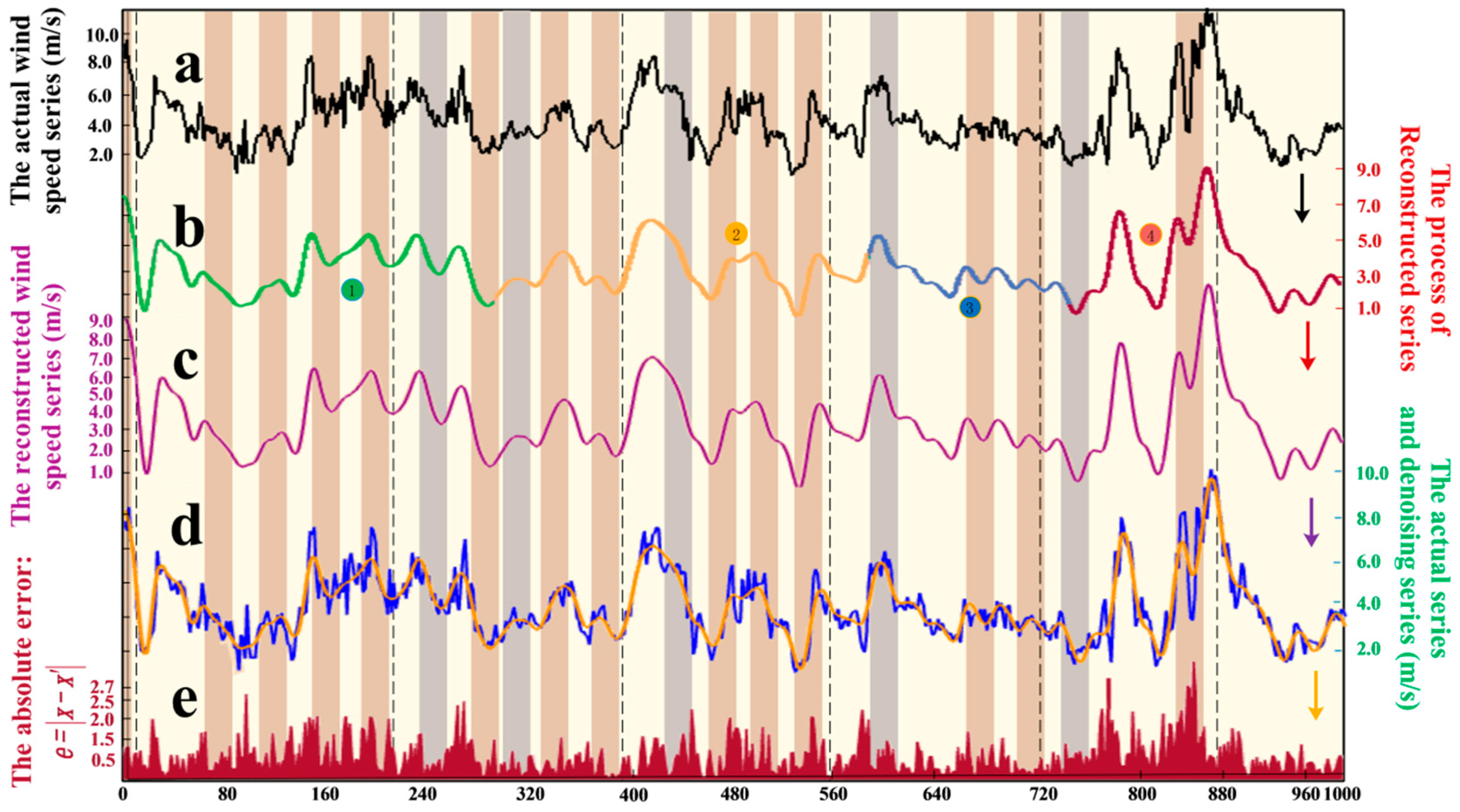
Table 7, respectively. Additionally, the results from Site 1 are displayed in Figure 5 and the absolute errors of the three sites are shown in Table 6 and Table 7. Using the four percentage error criteria, the improvement percentages between each set of algorithms are shown in Table 8 and Table 9.
From Table 6 and Table 7, we can see following:
(a)
Different forecasting algorithms have different forecasting results;
(b)
All the algorithms’ forecasting results from the three sites are effective. Examples are included in Figure 5;
(c)
For different seasons at the same site, the hybrid algorithms show strong forecasting stability;
(d)
Among the algorithms studied, the hybrid SSA–PSOSA–BP algorithm (see in Figure 6) obtained better accuracy than the others. Moreover, to further illustrate the quality of the proposed hybrid algorithm, four percentage error criterions are used in Table 5.
It can be analyzed in detail that:
(a)
When comparing the hybrid PSO–BP algorithm with the single BP algorithm, we can make a conclusion that the PSO selects excellent parameters to run BP model, but the prediction accuracy of PSO–BP is increased only slightly. From Table 6 and Table 7, in the spring, the three-step MAPE results of the PSO–BP and the BP are 7.2490% and 7.4083%, respectively. For the six-step, they are 9.0061% and 9.3530%, respectively.
(b)
When comparing the hybrid PSOSA–BP algorithm with the combined PSO–BP algorithm, the former combines the advantages of simulated annealing, and further optimizes the parameters; as a result, with respect to (a), the predicted quality rises again, but not particularly clearly. The specific upgrade percentages are provided in Table 8 and Table 9.
(c)
When comparing the hybrid SSA–APSOSA–BP algorithm with the hybrid PSOSA–BP algorithm, the former MAPE results are better than the latter. In other words, the forecasting quality of the new combined algorithm is better because of the higher accuracy when comparing it with the BP, PSO–BP, and PSOSA–BP algorithms.
(d)
The forecasting quality of the hybrid SSA–APSOSA–BP algorithm is better than that of the hybrid PSO–BP algorithm. The decreases in MAPE results in comparison with the PSO–BP and SSA–APSOSA–BP algorithm of three-step and six-step forecasts are 37.4439% and 36.9998% in Table 8 and Table 9 for the spring season, respectively.
(e)
When comparing the hybrid SSA–APSOSA–BP algorithm with the single BP algorithm, the accuracy of the wind speed forecasting, is improved more obviously. As an example, in Table 6, the three-step forecasting MAPE results for the latter are 9.4392%, 13.8388%, 13.0224%, and 11.4632%, respectively. However, for the former, the three-step forecasting MAPE results are 6.4101%, 9.0027%, 9.7494%, and 6.7077%, respectively.
(f)
From (a) to (e), the reasons include:
(1)
The combination of the SA algorithm and the PSO algorithm has increased the forecasting ability and accuracy of the single BP algorithm effectively.
(2)
The SSA algorithm removes the noise signal from the original wind speed data and, due to the APSOSA algorithm, the best initial weights and thresholds are given to optimize the BP algorithm, which can lead to high-precision forecasting results.
(3)
The scientific and rational data selection used in this paper is also one of the paramount reasons for the outstanding performance achieved.
In different seasons at the same site, the proposed algorithms’ forecasting qualities can also be different. This phenomenon indicates that wind speed can be affected by seasonal factors. In this paper, we also consider this factor, and the different seasons’ forecasting results are listed in Table 6 and Table 7. Table 10 and Table 11 are chosen as examples, and the detailed descriptions of this phenomenon are as follows:
(a)
Different sites can give different results. In Table 10, for the hybrid SSA–PSOSA–BP algorithm, the MAPE results of the three-step and six-step are 8.9477% and 10.8290%, respectively, at Site 1. However, for Sites 2 and 3, they are 7.9093% and 7.0741% vs. 7.9675% and 9.5219%, respectively.
(b)
In Table 11, for the hybrid SSA–APSOSA–BP algorithm in spring and winter, the MAPE of the three-step and six-step are 5.9362% and 6.8909% vs. 7.0652% and 8.8046%, respectively. However, in summer and autumn, they are 8.9720% and 10.7722% vs. 11.1259% and 12.7657%, respectively. Obviously, in spring and winter, the MAPE results are less than 9%, but in summer and autumn, the wind speed forecasting errors are all more than 10%, especially in autumn when they are close to 12%.
(c)
As can be clearly observed from the circumstances described above, geographical and seasonal factors must be considered in the wind speed prediction. From (b), it can be concluded that the prediction accuracy in spring and winter is better than that in summer and autumn. However, comparing with the other proposed algorithms, the forecasting errors of the hybrid algorithm are still effectively less.

4. Discussion

In this section, the bias–variance framework and the Diebold–Mariano (DM) are used to examine the accuracy, the stability, and the forecasting performance of the forecast models.

4.1. Bias–Variance Framework

In order to evaluate the different models’ accuracy and stability, in this subsection, we utilize the bias–variance framework, which includes bias and variance. The bias-variance framework can be shown as follows:
var = E [ ( y ^ y ) E ( y ^ y ) ] 2
B i a s 2 = E [ y ^ y ] 2 E [ y ^ E ( y ^ ) 2 ]
where y and y ^ are the observed values and the forecasting values respectively.
The higher the bias, the lower the forecasting accuracy. Similarly, the bigger the variance, the worse the prediction performance. The results of the models are shown in Table 12 and Table 13. Obviously, the bias and variance of the proposed hybrid model are smaller than the comparison models (GRNN, WNN, APSOSA–BPNN, etc.). In other words, the developed model possesses a higher accuracy and stability in wind-speed forecasting and performs much better than the comparison models in forecasting.

4.2. Statistical Hypothesis Testing

Hypothesis testing is a basic method of statistical inference, also called confirmatory data analysis. Its basic principle can be described as below: firstly, making some assumptions, then statistical reasoning, and lastly determining whether to reject or accept the hypothesis under a level of significance that is defined beforehand [4]. There are many commonly used methods of hypothesis testing such as T-test, F-test, rank and inspection, etc.
In this subsection, another hypothesis testing approach is employed to assess the models’ efficiency, called the Diebold–Mariano test [10]. The concrete content is described as follows:
H 0 : E [ ( L ( e t 1 ) ] = E [ ( L ( e t 2 ) ]
H 1 : E [ ( L ( e t 1 ) ] E [ ( L ( e t 2 ) ]
where the Loss function L is the function of the prediction error, e t 1 and e t 2 are the forecasting errors of the two comparison models.
Establishing the DM Statistics:
D M = d ¯ 2 π f ^ d ( 0 ) N d N ( 0 , 1 )
d ¯ = 1 N t   =   1 N [ L ( e t 1 ) L ( e t 2 ) ]
where 2 π f ^ d ( 0 ) represents a consistent estimator of the asymptotic variance, f ^ d ( 0 ) is the zero spectral density, and N is the length of forecasting results.
Comparing the calculated DM with the Z α / 2 , which can be found in the normal distribution table, the null hypothesis will be rejected if | D M | > | Z α / 2 | ; this means that under the significance level α, there is a significant difference between the two models (the proposed model and the compared models including WNN, GRNN, BPNN, etc.) in terms of their prediction performance. The concrete results are shown in Table 12 and Table 13.

4.3. Analysis

From Table 12 and Table 13, we can see that:
(a)
No matter the bias or the variance, the values of the proposed model are far smaller than those of the other five models, which means that the hybrid model has a higher accuracy and stability than the other five models.
(b)
The smallest value of the | D M | in both tables is 12.080501, which is much larger than the Z α / 2 ( Z 0.005 = 2.58 , Z 0.025 = 1.96 ); as a consequence, the null hypothesis can be rejected and the hybrid model observably outperforms the other five models.

5. Conclusions

With the conventional energy for electricity generation being quickly depleted, wind energy has become the most significant new type of green renewable energy available, and contains enormous power. However, due to the uncertainty of meteorological factors, it is still an extremely challenging task to forecast wind speed. In this paper, we put forward a novel hybrid SSA–APSOSA–BP model based on SSA and simulated annealing—adaptive particle swarm optimization algorithm (the specific process is given in Figure 6). From the above discussion and analysis, the conclusions are expressed as follows:
(1)
Among the three single prediction methods (WNN, GRNN, and BPNN), the best one is BPNN, which possesses a stronger prediction performance than the others (see Table 6 and Table 7).
(2)
In summer and autumn, wind speed forecasting errors are larger than in another two seasons because of the more complex features of wind speed in Penglai.
(3)
The experimental simulations indicate that the hybrid SSA–APSOSA–BP algorithm can perform better than the other five algorithms. There is no difference between the means of the forecasting series and the real series, and the accuracy of the wind speed forecasting results can be acceptable and credible within a reasonable range. The detailed reasons are provided in the above experimental simulations Section 3.3.
Overall, the proposed hybrid model adds a new viable option for wind speed forecasting, and the excellent performance and reasonable prediction accuracy reveal that they can be employed for time series forecasting, especially for wind-speed forecasting in some cases.

Acknowledgments

This work was financially supported by the National Natural Science Foundation of China (71171102).

Author Contributions

Pei Du and Yu Jin conceived and designed the experiments; Pei Du performed the experiments; Pei Du and Yu Jin analyzed the data; Kequan Zhang contributed reagents/materials/analysis tools; Pei Du wrote the paper.

Conflicts of Interest

The authors declare no conflict of interest.

Appendix A

Appendix A.1. Singular Spectrum Analysis (SSA)

Standard SSA is made up of two stages, decomposition and reconstruction, and each stage contains two steps.
Given a one-dimensional time series ( y 1 , , y N ) of length N, where L (integer) is the window length L ( 1 < L < N ) , and K is the number of lagged vectors ( K = N L + 1 ) , the specific steps are as follows:

Stage 1: Decomposition

In this stage, there are two steps: embedding and singular value decomposition (SVD).

Step 1: Embedding.

Form the trajectory matrix of the series X ( x 1 , , x K ) , which can be expressed by:
X = [ y 1 y 2 y 3 y k y 2 y 3 y 4 y k + 1 y 3 y 4 y 5 y k + 2 y L y L + 1 y L + 2 y N ] L × K
what is noteworthy is that T i j , an element of X , stands for the i-th line and the j-th column, which possess the characteristic T i j = T i     1 , j   +   1 .

Step 2: SVD

Calculate the matrix S ( S = X X T ) and the eigenvalues λ 1 , ... , λ L . of S , which are the decreasing sequence λ 1 ... λ L 0 . Furthermore, U 1 ,   ...   , U L represent the corresponding orthogonal eigenvectors of the matrix S . Lastly, the SVD of the trajectory matrix X can be expressed through Equation (A2):
X = X 1 + ... + X d
where X i = λ i U i   v i T having rank 1, d = { i , such that λ i > 0 } and v i = X T U i / λ i   ( i = 1 , ... , d ) are elementary matrices. The group ( λ i , U i , v i T ) will be known as the i-th eigentriple (abbreviated as ET).

Stage 2: Reconstruction

This stage is subdivided into two steps: grouping and diagonal averaging.

Step 3: Grouping

Firstly, we divide the abovementioned matrix X i into m groups, which are different from each other, and then add up the total matrices in each group. Next, let I = { i 1 , ... , i p } , i 1 , ... , i p stand for the indices of each group, and then the I-th group resultant matrix X I can be described as below: X I = X i 1 + ... + X i p . Here, we divide I = { 1 , ... , d } into two different subsets I 1 = { 1 , , r } , and I 1 = { r + 1 , , d } , then X I can be written as Equation (A3):
X I = X I 1 + ... + X Im

Step 4: Diagonal Averaging

In this step, transform the mentioned grouped matrix X I into a new series of length N and set X = ( x i j ) L   ×   K , if L > K ,   x i j * = x j i , otherwise x i j * = x i j . Finally, ( f 1 , , f N ) can be converted to a series by Equation (A4):
f k = { 1 k + 1 m = 1 k + 1 y m , k m + 2 0 k L * 1 1 L * m = 1 L * y m , k m + 2 L * k k * 1 k + 1 m = 1 k + 1 y m , k m + 2 k * k N 1
in which L * = m i n ( L , k ) ,   k * = m a x ( L , k ) . In this method, the first r main constituents can be viewed as the most vital information, the rest are considered the noise of the original data.

Appendix B

Appendix B.1. Particle Swarm Optimization

The core of the PSO is learning the foraging behavior of birds. Assuming a forest setting, the birds do not know the position of the food. However, they can receive some information concerning the food location, and then search for the nearest food. These birds can be treated as the particles in the PSO algorithm; each particle can be regarded as a candidate solution in search space (n dimensions). Each particle continues to search for a better position by adjusting its velocity v i ( t ) = [ v i 1 , v i 2 , , v i n ] T ; in light of their flying memory, birds decide on the personal best (pbest) solution. Finally, the global best (gbest) solution can be obtained by comparing the personal best solutions with each other. The updated position and velocity rules are defined as Equations (B1) and (B2):
v i ( t + 1 ) = ω ( t ) v i ( t ) + c 1 r 1 ( p b e s t x i ( t ) ) + c 2 r 2 ( g b e s t x i ( t ) )
x i ( t + 1 ) = x i ( t ) + v i ( t + 1 )
where t is the current iteration, ω stands for the inertia weight, the particle position is x i ( t ) = [ x i 1 , x i 2 , , x i n ] , r 1 and r 2 are random numbers in [0, 1], and the learning factors c 1 and c 2 stand for weights of pbest and gbest, respectively.

Appendix B.2. Back Propagation Neural Network (BPNN)

We determined the input vector by normalizing each input value by Equation (B3):
V = { V i } = x i x i min x i max x i min  
where x i min and x i max are the minimal and maximal value of each input factor, respectively.
  • Step 1: Calculate the outputs of all hidden layer nodes. Based on the input vector X , the weight ω i j , which is between the input layer and the hidden layer, and the hidden layer threshold O, compute outputs H of the whole hidden layer node in Equation (B4). S is the number of the hidden layer nodes.
    H j = G ( i = 1 n ω i j x i a j ) ,   j = 1 , , s
    G ( x ) = 1 1 + e x
  • Step 2: Make a calculation about the output data of neural network, according to outputs H of all hidden layer nodes, the weights ω i j , and the weight λ using Equation (B6):
    O k = j = 1 l H j ω j k λ k ,   k = 1 , , p
  • Step 3: Depending on the predicted output O and the expected output Y , calculate the error using Equation (B7):
    e k = Y k O k ,   k = 1 , , p
  • Step 4: Update the weights by using the predicted error and the weights ω i j   ω j k in Equations (B8) and (B9):
    ω i j = ω i j + η H j ( 1 H j ) x i k = 1 m ω i k e k ,   i = 1 , , n ;   j = 1 , , s
    ω i j = ω i j + η H j e k ,   k = 1 , , p ,   j = 1 , , s
  • Step 5: Update the thresholds using Equations (B10) and (B11):
    a j = a j + η H j ( 1 H j ) k = 1 m ω j k e k ,   j = 1 , , s
    λ k = λ k + e k ,   k = 1 , , p
  • Step 6: Repeat the above steps until the errors reach the preset accuracy.

Appendix B.3. Simulated Annealing (SA)

Definition 1. 
The main steps of simulated annealing are given as follows:
  • Step 1: Parameter initialization. Set the initialization temperature T 0 as high as feasible and randomly generate initial solution x 0 .
  • Step 2: Repeat the following until equilibrium temperature is reached: T ( k )   ( k = 1 , .. , L )   ( L is the number of iteration).
    (1)
    Generating the new solution x in the range of the solution X , set objective function F ( x ) and calculate F ( x ) and F ( x ) :
    Δ F = F ( x ) F ( x )
    (2)
    If Δ F < 0 , accept x as the new solution, else accept the worse solution x as the new one with the probability in Equation (B13):
    P = e Δ F ( x ) / K T
    where K is the Boltzmann Constant.
  • Step 3: Repeat step 2 until the declining temperature reaches zero or the pre-set temperature T.

References

  1. Xiao, L.; Wang, J.; Dong, Y.; Wu, J. Combined forecasting models for wind energy forecasting: A case study in China. Renew. Sustain. Energy Rev. 2015, 44, 271–288. [Google Scholar] [CrossRef]
  2. Khatib, H. IEA World Energy Outlook 2010—A comment. Energy Policy 2011, 39, 2507–2511. [Google Scholar] [CrossRef]
  3. Li, D.H.W.; Liu, Y.; Joseph, C. Zero energy buildings and sustainable development implications—A review. Energy 2013, 54, 1–10. [Google Scholar] [CrossRef]
  4. Wang, J.Z.; Wang, Y.; Jiang, P. The study and application of a novel hybrid forecasting model–A case study of wind speed forecasting in China. Appl. Energy 2015, 143, 472–488. [Google Scholar] [CrossRef]
  5. Cassola, F.; Burlando, M. Wind speed and wind energy forecast through Kalman filtering of Numerical Weather Prediction model output. Appl. Energy 2012, 99, 154–166. [Google Scholar] [CrossRef]
  6. Calif, R.; Schmitt, F.G.; Huang, Y. The scaling properties of the turbulent wind using Empirical Mode Decomposition and arbitrary order Hilbert Spectral Analysis. In Wind Energy-Impact of Turbulence; Springer: Oldenburg, Germany, 2014; pp. 43–49. [Google Scholar]
  7. Liu, H.; Tian, H.; Li, Y. An EMD-recursive ARIMA method to predict wind speed for railway strong wind warning system. J. Wind Eng. Ind. Aerodyn. 2015, 141, 27–38. [Google Scholar] [CrossRef]
  8. Ye, R.; Suganthan, P.N.; Srikanth, N. A Comparative Study of Empirical Mode Decomposition-Based Short-Term Wind Speed Forecasting Methods. IEEE Trans. Sustain. Energy 2015, 6, 236–244. [Google Scholar]
  9. Hassani, H.; Webster, A.; Silva, E.S.; Heravi, S. Forecasting US tourist arrivals using optimal singular spectrum analysis. Tour. Manag. 2015, 46, 322–335. [Google Scholar] [CrossRef]
  10. Heng, J.; Wang, C.; Zhao, X.; Xiao, L. Research and application based on adaptive boosting strategy and modified CGFPA algorithm: A case study for wind speed forecasting. Sustainability 2016, 8, 235. [Google Scholar] [CrossRef]
  11. Ma, L.; Luan, S.Y.; Jiang, C.W.; Liu, H.L.; Zhang, Y. A review on the forecasting of wind speed and generated power. Renew. Sustain. Energy Rev. 2009, 13, 915–920. [Google Scholar]
  12. Watson, S.J.; Landberg, L.; Halliday, J.A. Application of wind speed forecasting to the integration of wind energy into a large scale power system. IET Proc. Gener. Transm. Distr. 1994, 141, 357–362. [Google Scholar] [CrossRef]
  13. Landberg, L. Short-term prediction of the power production from wind farms. J. Wind Eng. Industr. Aerodyn. 1999, 80, 207–220. [Google Scholar] [CrossRef]
  14. Hong, J.S. Evaluation of the high-resolution model forecasts over the Taiwan area during GIMEX. Weather Forecast. 2003, 18, 836–846. [Google Scholar] [CrossRef]
  15. Chen, K.; Yu, J. Short-term wind speed prediction using an unscented Kalman filter based state-space support vector regression approach. Appl. Energy 2014, 113, 690–705. [Google Scholar] [CrossRef]
  16. Douak, F.; Melgani, F.; Benoudjit, N. Kernel ridge regression with active learning for wind speed prediction. Appl. Energy 2013, 103, 328–340. [Google Scholar] [CrossRef]
  17. Morales, J.M.; Mínguez, R.; Conejo, A.J. A methodology to generate statistically dependent wind speed scenarios. Appl. Energy 2010, 87, 843–855. [Google Scholar] [CrossRef]
  18. Erdem, E.; Shi, J. ARMA based approaches for forecasting the tuple of wind speed and direction. Appl. Energy 2011, 88, 1405–1414. [Google Scholar] [CrossRef]
  19. Liu, H.; Erdem, E.; Shi, J. Comprehensive evaluation of ARMA-GARCH (-M) approaches for modeling the mean and volatility of wind speed. Appl. Energy 2011, 88, 724–732. [Google Scholar] [CrossRef]
  20. Torres, J.L.; García, A.; Blas, M.D.; De Francisco, A. Forecast of hourly average wind speed with ARMA models in Navarre (Spain). Sol. Energy 2005, 79, 65–77. [Google Scholar] [CrossRef]
  21. Kamal, L.; Jafri, Y.Z. Time series models to simulate and forecast hourly averaged wind speed in Quetta, Pakistan. Sol. Energy 1997, 61, 23–32. [Google Scholar] [CrossRef]
  22. Liu, H.; Chen, C.; Tian, H.; Li, Y.-F. A hybrid model for wind speed prediction using empirical mode decomposition and artificial neural networks. Renew. Energy 2012, 48, 545–556. [Google Scholar] [CrossRef]
  23. Kavasseri, R.G.; Seetharaman, K. Day-ahead wind speed forecasting using f-ARIMA models. Renew. Energy 2009, 34, 1388–1393. [Google Scholar] [CrossRef]
  24. Xu, X.; Qi, Y.; Hua, Z. Forecasting demand of commodities after natural disasters. Expert Syst. Appl. 2010, 37, 4313–4317. [Google Scholar] [CrossRef]
  25. Mohandes, M.A.; Rehman, S.; Rahman, S.M. Spatial estimation of wind speed. Int. J. Energy Res. 2012, 36, 545–552. [Google Scholar] [CrossRef]
  26. Blonbou, R. Very short-term wind power forecasting with neural networks and adaptive Bayesian learning. Renew. Energy 2011, 36, 1118–1124. [Google Scholar] [CrossRef]
  27. Barbounis, T.; Theocharis, J. Locally recurrent neural networks for long-term wind speed and power prediction. Neurocomputing 2006, 69, 466–496. [Google Scholar] [CrossRef]
  28. Barbounis, T.; Theocharis, J. Locally recurrent neural networks for wind speed prediction using spatial correlation. Inf. Sci. 2007, 177, 5775–5797. [Google Scholar] [CrossRef]
  29. Guo, Z.H.; Zhao, W.G.; Lu, H.Y.; Wang, J.Z. Multi-step forecasting for wind speed using a modified EMD-based artificial neural network model. Renew. Energy 2012, 37, 241–249. [Google Scholar] [CrossRef]
  30. Babu, N.R.; Mohan, B.J. Fault classification in power systems using EMD and SVM. Ain Shams Eng. J. 2015. [Google Scholar] [CrossRef]
  31. Sfetsos, A. A novel approach for the forecasting of mean hourly wind speed time series. Renew. Energy 2002, 27, 163–174. [Google Scholar] [CrossRef]
  32. Pandian, S.C.; Duraiswamy, K.; Rajan, C.C.A.; Kanagaraj, N. Fuzzy approach for short term load forecasting. Electr. Power Syst. Res. 2006, 76, 541–548. [Google Scholar] [CrossRef]
  33. Zhao, J.; Guo, Z.H.; Su, Z.Y.; Zhao, Z.-Y.; Xiao, X.; Liu, F. An improved multi-step forecasting model based on WRF ensembles and creative fuzzy systems for wind speed. Appl. Energy 2016, 162, 808–826. [Google Scholar] [CrossRef]
  34. Sharafi, M.; ElMekkawy, T.Y. A dynamic MOPSO algorithm for multiobjective optimal design of hybrid renewable energy systems. Int. J. Energy Res. 2014, 38, 1949–1963. [Google Scholar] [CrossRef]
  35. Zhao, S.Z.; Suganthan, P.N.; Pan, Q.K.; Tasgetiren, M.F. Dynamic multi-swarm particle swarm optimizer with harmony search. Expert Syst. Appl. 2011, 38, 3735–3742. [Google Scholar] [CrossRef]
  36. Chyan, G.S.; Ponnambalam, S.G. Obstacle avoidance control of redundant robots using variants of particle swarm optimization. Robot. Comput. Integr. Manuf. 2012, 28, 147–153. [Google Scholar]
  37. Bingül, Z.; Karahan, O. Dynamic identification of Staubli RX-60 robot using PSO and LS methods. Expert Syst. Appl. 2011, 38, 4136–4149. [Google Scholar] [CrossRef]
  38. Vasumathi, B.; Moorthi, S. Implementation of hybrid ANN–PSO algorithm on FPGA for harmonic estimation. Eng. Appl. Artif. Intell. 2012, 25, 476–483. [Google Scholar] [CrossRef]
  39. Damodaran, P.; Vélez-Gallego, M.C. A simulated annealing algorithm to minimize makespan of parallel batch processing machines with unequal job ready times. Expert Syst. Appl. 2012, 39, 1451–1458. [Google Scholar] [CrossRef]
  40. Patil, M.; Nikumbh, P.J. Pair-wise testing using simulated annealing. Procedia Technol. 2012, 4, 778–782. [Google Scholar] [CrossRef]
  41. Garcia-Lopez, N.P.; Sanchez-Silva, M.; Medaglia, A.L.; Chateauneuf, A. A hybrid topology optimization methodology combining simulated annealing and SIMP. Comput. Struct. 2011, 89, 1512–1522. [Google Scholar] [CrossRef]
  42. Popović, Ž.N.; Kerleta, V.D.; Popović, D.S. Hybrid simulated annealing and mixed integer linear programming algorithm for optimal planning of radial distribution networks with distributed generation. Electr. Power Syst. Res. 2014, 108, 211–222. [Google Scholar] [CrossRef]
  43. Akar, S.A.; Kara, S.; Latifoğlu, F.; Bilgiç, V. Investigation of the noise effect on fractal dimension of EEG in schizophrenia patients using wavelet and SSA-based approaches. Biomed. Signal Process. Control 2015, 18, 42–48. [Google Scholar] [CrossRef]
  44. Kennedy, J. Particle swarm optimization. In Encyclopedia of Machine Learning; Springer: New York, NY, USA, 2011; pp. 760–766. [Google Scholar]
  45. Rumelhart, D.E.; Hinton, G.E.; Williams, R.J. Learning representations by back-propagating errors. Nature 1986, 323, 533–536. [Google Scholar] [CrossRef]
  46. Qin, S.; Liu, F.; Wang, J.; Song, Y. Interval forecasts of a novelty hybrid model for wind speeds. Energy Rep. 2015, 1, 8–16. [Google Scholar] [CrossRef]
  47. Kirkpatrick, S. Optimization by simulated annealing: Quantitative studies. J. Stat. Phys. 1984, 34, 975–986. [Google Scholar] [CrossRef]
Figure 1. Original wind speed series and the decomposed series by SSA.
Sustainability 08 00754 g001
Figure 2. The conceptual diagram of the Roulette Wheel Selection Strategy.
Sustainability 08 00754 g002
Figure 3. The flowchart of the proposed hybrid algorithm.
Sustainability 08 00754 g003
Figure 4. The study area, Penglai in Shandong province, eastern China.
Sustainability 08 00754 g004
Figure 5. Rolling forecasting results of different models at the three study sites.
Sustainability 08 00754 g005
Figure 6. The flowchart of the proposed model.
Sustainability 08 00754 g006
Table 1. The experimental parameters of BPNN.
Experimental ParametersDefault Value
neuron number in the input layer4
neuron number in the hidden layer8
neuron number in the hidden layer1
the learning velocity0.1
the maximum number of trainings1500
training requirements precision0.0001
Table 2. A rudimentary SA-APSO algorithm is outlined as follows.
  Algorithm: SA-APSO
Input:
x s ( 0 ) = ( x ( 0 ) ( 1 ) , x ( 0 ) ( 2 ) , , x ( 0 ) ( l ) ) a   s e q u e n c e   o f   t r a i n i n g   d a t a .
x p ( 0 ) = ( x ( 0 ) ( l + 1 ) , x ( 0 ) ( l + 2 ) , , x ( 0 ) ( l + n ) ) a   s e q u e n c e   o f   v e r i f y i n g   d a t a .
Output:
Pg—the value of x with the best fitness value in population of particles
Parameters:
Itermax—the maximum number of iterations
n—the number of particles
Fi—the fitness function of particle i
xi—particle i
g—the current iteration number
d—the number of dimension
1: /* Set the parameters of PSO and SA. */
2: /* Initialize population of n particle xi (i = 1, 2,..., n) randomly */
3: FOR EACH i: 1 ≤ in DO
4: Evaluate the corresponding fitness function Fi
5: END FOR
6: /* Determine the global best position */
7: FOR EACH i: 1 ≤ in DO
8: Determine the global best position Pg by using F(xi).
9: {F(Pg), g}=max{(F(P1), …, F (PN)}
10: END FOR
11: WHILE (g < Itermax) DO
12: /* Determine the initial temperature. */
13: FOR EACH i: 1 ≤ in DO
14: T0=−F(Pi)/ln(0.2)
15: END FOR
16: FOR EACH i = 1:n DO
17: FOR EACH j = 1:n DO
18: /* Calculate the probability P(Pi) */
19: /* Judge the relationship of the probability P(Pi) and rand () */
20: IF (P(Pi) > rand()) THEN
21: Pg = Pg = Pi
22: END IF
23: /* Update the velocity and position of each particle */
24: FOR EACH i: 1 ≤ in DO
25: vi(t + 1) = w(t)vi(t) + c1r1(pixi(t)) + c2r2(pgxi(t));
26: xi(t + 1)= xi(t) + vi(t + 1);
27: END FOR
28: /* Evaluate the new position Pi and fitness function F(Pi). */
29: FOR EACH i: 1 ≤ in DO
30: Evaluate the corresponding fitness function F(Pi)
31: END FOR
32: /* Judge the relationship of fitness function F(Pi) and F (Pi). */
33: IF (F(Pi) > F (Pi)) THEN
34: Pi = Pi and F (Pi) = F(Pi)
35: END IF
36: /* Judge the relationship of fitness function F(Pi) and F(Pg). */
37: IF (F (Pi) > F (Pg)) THEN
38: Pg = Pi and F (Pg) = F(Pi)
39: END IF
40: /* Cooling the temperature */
41: FOR EACH i: 1 ≤ in DO
42: Ti + 1 = a × Ti
43: END FOR
44: END FOR
45: END FOR
46: END WHILE
47: RETURN Pg
Table 3. The experimental parameters of APSOSA.
Experimental ParametersDefault Value
The population size: N30
maximum initial velocity2
minimum initial velocity−2
the learning factor: C12.2
the learning factor: C21.8
The evolution number: M200
Table 4. Four metric rules.
MetricDefinitionEquation
AEThe average forecast error of i times forecast results AE = 1 N i = 1 N ( y i y ^ i )
MAEThe average absolute forecast error of i times forecast results MAE = 1 N i = 1 N | y i y ^ i |
RMSEThe root average of the prediction error squares RMSE = 1 N i = 1 N ( y i y ^ i ) 2
MAPEThe average of absolute error MAPE = 1 N i = 1 N | y i y ^ i y i | × 100 %
Table 5. Four metric rules.
MetricDefinitionEquation
Q AE The percentage error of AE Q AE = | AE 1 AE 2 AE 1 |
Q MAE The percentage error of MAE Q MAE = | MAE 1 MAE 2 MAE 1 |
Q RMSE The percentage error of RMSE Q RMSE = | RMSE 1 RMSE 2 RMSE 1 |
Q MAPE The percentage error of MAPE Q MAPE = | MAPE 1 MAPE 2 MAPE 1 |
Table 6. Comparison of errors of rolling three-step (half an hour ahead) forecasts.
IndexesSite 1Site 2Site 3
SpringSummerAutumnWinterSpringSummerAutumnWinterSpringSummerAutumnWinter
AE
WNN−0.05380.2344−0.01930.07330.12360.28130.0000−0.02250.06540.25840.08630.0065
GRNN−0.2328−0.11340.0624−0.1384−0.33210.6803−0.12140.10040.14470.23020.2108−0.0541
BPNN−0.15620.12300.04140.12030.04310.4185−0.2744−0.0795−0.19860.0094−0.09270.0843
PSO–BP−0.11060.3070−0.1049−0.06520.02420.3804−0.1223−0.0294−0.0670−0.0296−0.06190.0137
APSOSA–BP−0.11810.0890−0.05710.00240.1030.3321−0.11110.0022−0.03960.0774−0.07790.0099
Proposed model−0.01320.0223−0.0014−0.01120.01360.0343−0.0415−0.0007−0.01250.0078−0.01980.0012
MAE
WNN0.86900.83880.74170.79270.81351.13420.56760.71510.74871.15150.56290.6335
GRNN0.73940.69620.68730.63050.71571.08500.47130.58110.61380.90310.46730.5075
BPNN0.72330.70070.59900.63110.63881.03170.50500.53350.58250.79960.42930.4833
PSO–BP0.70110.76120.57770.58840.62330.94360.46640.52760.56340.79450.42450.4726
APSOSA–BP0.69750.65450.55490.57610.62300.91330.45710.51430.55140.79380.42430.4681
Proposed model0.44930.41510.34370.34890.42110.53120.32890.33510.41520.53120.31710.2900
RMSE
WNN1.15301.16830.97911.02441.05911.57570.73160.93830.97781.59870.75640.8070
GRNN0.97840.94790.99990.81470.91651.60590.60520.76800.80381.27590.63330.6539
BPNN0.96240.94780.83430.81450.84541.63640.65430.71690.76371.18380.58120.6207
PSO–BP0.93811.10050.77350.76280.82671.39670.60050.69950.74531.16120.57470.6242
APSOSA–BP0.93170.91340.72680.74720.83081.31910.58850.69270.73451.15850.57450.6155
Proposed model0.59180.54540.46370.44660.55310.70080.41770.43360.54110.72970.40680.3688
MAPE
WNN12.829919.212324.218016.29789.497815.105420.822516.500511.687719.470616.778914.4603
GRNN11.480417.643221.598513.59948.577612.841318.548113.09709.666115.088913.368612.5040
BPNN11.093016.860718.538013.53357.408312.615819.645312.40609.439213.838813.022411.4632
PSO–BP10.61416.48518.388612.31067.249011.938317.811112.12869.026613.764112.924111.2132
APSOSA–BP10.534115.702518.216512.24187.139711.615417.402211.63528.513313.567812.830711.0325
Proposed model6.639710.665911.37237.11284.75897.247312.25597.37506.41019.00279.74946.7077
Table 7. Comparison of errors of rolling six-step (one hour ahead) forecasts.
IndexesSite 1Site 2Site 3
SpringSummerAutumnWinterSpringSummerAutumnWinterSpringSummerAutumnWinter
AE
WNN−0.16120.32950.2508−0.06310.11070.1754−0.0188−0.0603−0.04580.0132−0.23710.0187
GRNN−0.2724−0.18500.0224−0.1431−0.46680.8426−0.18090.17340.44930.3922−0.11920.0486
BPNN0.1676−0.3026−0.0800−0.2177−0.1111−0.40450.44970.11200.25480.00880.1565−0.1241
PSO–BP0.1473−0.53590.18450.0699−0.0914−0.46420.20820.00880.02620.07370.10420.0238
APSOSA–BP0.1399−0.14350.0799−0.0624−0.2008−0.37630.1782−0.01850.0301−0.12830.12220.0253
Proposed model0.0595−0.09260.02350.0484−0.0067−0.15300.05570.01540.0285−0.00400.01790.0175
MAE
WNN0.98330.97700.83320.87600.95991.28530.61760.77970.83321.25980.65250.7299
GRNN0.85360.81510.81370.75000.89601.28910.55540.69930.81271.08770.54140.6148
BPNN0.83250.9580.77760.79540.79121.18870.65590.64170.71621.01570.54500.5919
PSO–BP0.83271.03440.74300.73760.75761.14110.55420.61720.68481.00460.53430.5540
APSOSA–BP0.81850.79550.67770.71170.76881.09200.53730.61430.66910.99460.53110.5542
Proposed model0.56530.50780.42410.40860.45820.63060.36110.40610.45840.66430.35020.3678
RMSE
WNN1.28231.34061.11231.13491.21841.79780.78931.03011.08231.76890.85570.9242
GRNN1.11251.11311.12220.98381.14281.88270.71750.92071.06581.52770.72820.7770
BPNN1.09411.30321.11541.03361.03261.84270.82880.84490.93691.48130.73450.7541
PSO–BP1.10121.49001.02440.96080.98981.66650.71320.81720.90731.46480.72380.7195
APSOSA–BP1.08281.10630.89870.94231.01261.57840.69410.81510.89391.42940.71930.7202
Proposed model0.76030.73600.55390.52950.60670.95610.45790.53220.60160.92690.45590.4783
MAPE
WNN15.677422.154226.583818.127311.431317.463622.755518.379313.977421.495521.041116.5445
GRNN13.517422.026925.500816.462211.023415.785622.482815.679612.160317.685317.440614.5046
BPNN13.214422.322723.510816.78419.353015.573026.664915.118911.877817.386917.541013.8192
PSO–BP13.157921.626523.125415.50459.006114.889322.248314.556511.135917.380217.086913.4498
APSOSA–BP12.705719.688322.307615.00018.947214.632221.267414.241310.536316.836516.75613.1057
Proposed model8.289512.400413.79758.82855.23388.276113.56999.21677.149311.640110.92968.3685
Table 8. Improvement percentages among different forecasting models of rolling three-step (half an hour ahead) forecasts.
IndexesSite 1Site 2Site 3
SpringSummerAutumnWinterSpringSummerAutumnWinterSpringSummerAutumnWinter
QAE
BP vs. Proposed model91.547081.8408103.3182109.303568.345391.793084.880899.114432.090634.945925.133641.4849
PSO vs. Proposed model88.061892.723098.690282.818543.676590.970666.077797.608928.986634.592924.564240.1803
APSOSA vs. Proposed model88.821974.906197.5929564.831286.754189.656262.6562131.457624.704933.646624.015139.2005
QMAE
BP vs. Proposed model37.881940.759242.621044.715634.079548.512234.871337.188428.721033.566826.135639.9959
PSO vs. Proposed model35.915045.467740.505540.703632.440243.705029.481136.486026.304633.140325.300438.6373
APSOSA vs. Proposed model35.584236.577538.060939.437632.407741.837328.046434.843524.700833.081425.265138.0474
QRMSE
BP vs. Proposed model38.507942.456244.420545.168834.575357.174336.160839.517429.147638.359530.006940.5832
PSO vs. Proposed model36.915050.440740.051741.452533.095449.824630.441338.012927.398437.159829.215240.9164
APSOSA vs. Proposed model36.481740.289036.199840.230233.425646.872929.022937.404426.330837.013429.190640.0812
QMAPE
BP vs. Proposed model40.145136.741138.654147.443035.762642.553837.614140.553032.090634.945925.133641.4849
PSO vs. Proposed model37.443935.299438.155742.222234.350939.293731.189539.193328.986634.592924.564240.1803
APSOSA vs. Proposed model36.969532.075137.571441.897433.345937.606129.572736.614824.704933.646624.015139.2005
Table 9. Improvement percentages among different forecasting models of rolling six-step (one hour ahead) forecasts.
IndexesSite 1Site 2Site 3
SpringSummerAutumnWinterSpringSummerAutumnWinterSpringSummerAutumnWinter
QAE
BP vs. Proposed model64.512469.3882129.3627122.253193.947862.180887.619486.228839.809633.052537.691139.4429
PSO vs. Proposed model59.597782.713687.272730.728092.646467.041673.261974.692135.799533.026736.035237.7797
APSOSA vs. Proposed model57.486535.469270.6258177.613596.652959.347268.7603183.326232.146030.863934.772036.1461
QMAE
BP vs. Proposed model32.096146.993745.460448.629642.088046.950544.945936.715035.995534.596835.743137.8611
PSO vs. Proposed model32.112450.908742.920644.604139.519544.737534.843034.202933.060733.874234.456333.6101
APSOSA vs. Proposed model30.934636.165937.420742.588240.400642.252732.793633.892231.490133.209334.061433.6341
QRMSE
BP vs. Proposed model30.509143.523650.340748.771341.245448.114244.751437.010335.788237.426637.930636.5734
PSO vs. Proposed model30.957150.604045.929344.889738.704842.628335.796434.875233.693436.721737.013033.5233
APSOSA vs. Proposed model29.783933.471938.366543.807740.084939.426034.029734.707432.699435.154636.618933.5879
QMAPE
BP vs. Proposed model37.269244.449441.314247.399644.041546.856149.109539.038639.809633.052537.691139.4429
PSO vs. Proposed model36.999842.661140.336243.058541.886144.415839.007036.683335.799533.026736.035237.7797
APSOSA vs. Proposed model34.757637.016438.148941.143741.503543.439136.193935.281932.146030.863934.772036.1461
Table 10. Average errors of the different rolling forecasting models at the three sites.
BPPSO–BPAPSOSA–BPSSA–APSOSA–BP
AreaAverage3-Step6-Step3-Step6-Step3-Step6-Step3-Step6-Step
Site 1AE (m/s)−0.0321−0.1082−0.0066−0.03360.02100.00350.00090.0097
MAE (m/s)0.66350.84090.65710.83690.62080.75090.38930.4765
RMSE (m/s)0.88981.13660.89371.14410.82981.00750.51190.6449
MAPE (%)15.006318.958014.449618.353614.173717.42548.947710.8290
Site 2AE (m/s)−0.02690.0115−0.0632−0.0847−0.0816−0.1044−0.0014−0.0222
MAE (m/s)0.67730.81940.64020.76750.62690.75310.40410.4640
RMSE (m/s)0.96331.13730.88091.04670.85781.02510.52630.6382
MAPE (%)13.018916.677512.281815.175111.948114.77207.90939.0741
Site 3AE (m/s)0.04940.07400.03620.05700.00760.01230.00580.0150
MAE (m/s)0.57370.71720.56380.69440.55940.68730.38840.4602
RMSE (m/s)0.78740.97670.77640.95390.77080.94070.51160.6157
MAPE (%)11.940915.156211.732014.763211.486114.30867.96759.5219
Table 11. Average errors of the different rolling forecasting models in different seasons.
BPPSO–BPAPSOSA–BPSSA–APSOSA–BP
SeasonAverage3-Step6-Step3-Step6-Step3-Step6-Step3-Step6-Step
SpringAE (m/s)0.10390.10380.05110.02740.0182−0.0100.00400.0271
MAE (m/s)0.64820.78000.62930.75840.62400.75210.42850.4940
RMSE (m/s)0.85721.02120.83670.99940.83230.99640.56200.6562
MAPE (%)9.313511.48178.963211.1008.729010.7295.93626.8909
SummerAE (m/s)−0.1836−0.2328−0.2193−0.3088−0.166−0.2160−0.021−0.083
MAE (m/s)0.84401.05410.83311.06000.78720.96070.49250.6009
RMSE (m/s)1.25601.54241.21951.54041.13031.37140.65860.8730
MAPE (%)14.438418.427514.062517.96513.62817.05238.972010.772
AutumnAE (m/s)0.10860.17540.09640.16560.08200.12680.02090.0324
MAE (m/s)0.51110.65950.48950.61050.47880.58200.32990.3785
RMSE (m/s)0.68990.89290.64960.82050.62990.77070.42940.4892
MAPE (%)17.068622.572216.374620.820216.149820.110311.125912.7657
WinterAE (m/s)−0.0417−0.07660.02700.0342−0.0048−0.01850.00360.0271
MAE (m/s)0.54930.67630.52950.63630.51950.62670.32470.3942
RMSE (m/s)0.71740.87750.69550.83250.68510.82590.41630.5133
MAPE (%)12.467615.240711.884114.503611.636514.11577.06528.8046
Table 12. Bias–variance and Diebold–Mariano test of different models (half an-hour ahead).
Different ModelsBias–Variance FrameworkDiebold–Mariano Statistic
Bias2Var
WNN0.0197501.18634015.016983 *
GRNN0.0674410.84987912.978130 *
BPNN0.0307990.82029713.903475 *
PSO–BP0.0243530.75802413.244862 **
APSOSA–BP0.0143420.70607412.841336 **
Proposed model0.0003750.278953
* is the 1% significance level; ** is the 5% significance level.
Table 13. Bias–variance and Diebold–Mariano test of different models (one hour ahead).
Different ModelsBias–Variance FrameworkDiebold–Mariano Statistic
Bias2Var
WNN0.0256121.49710716.081645 *
GRNN0.1243551.17029513.999003 *
BPNN0.0557631.21175712.749358 *
PSO–BP0.0527171.14423412.080501 **
APSOSA–BP0.0247911.02905812.739267 **
Proposed model0.0036050.424805
* is the 1% significance level; ** is the 5% significance level.

