
Dynamic Ecological Risk Assessment and Management of Land Use in the Middle Reaches of the Heihe River Based on Landscape Patterns and Spatial Statistics

Abstract
:1. Introduction
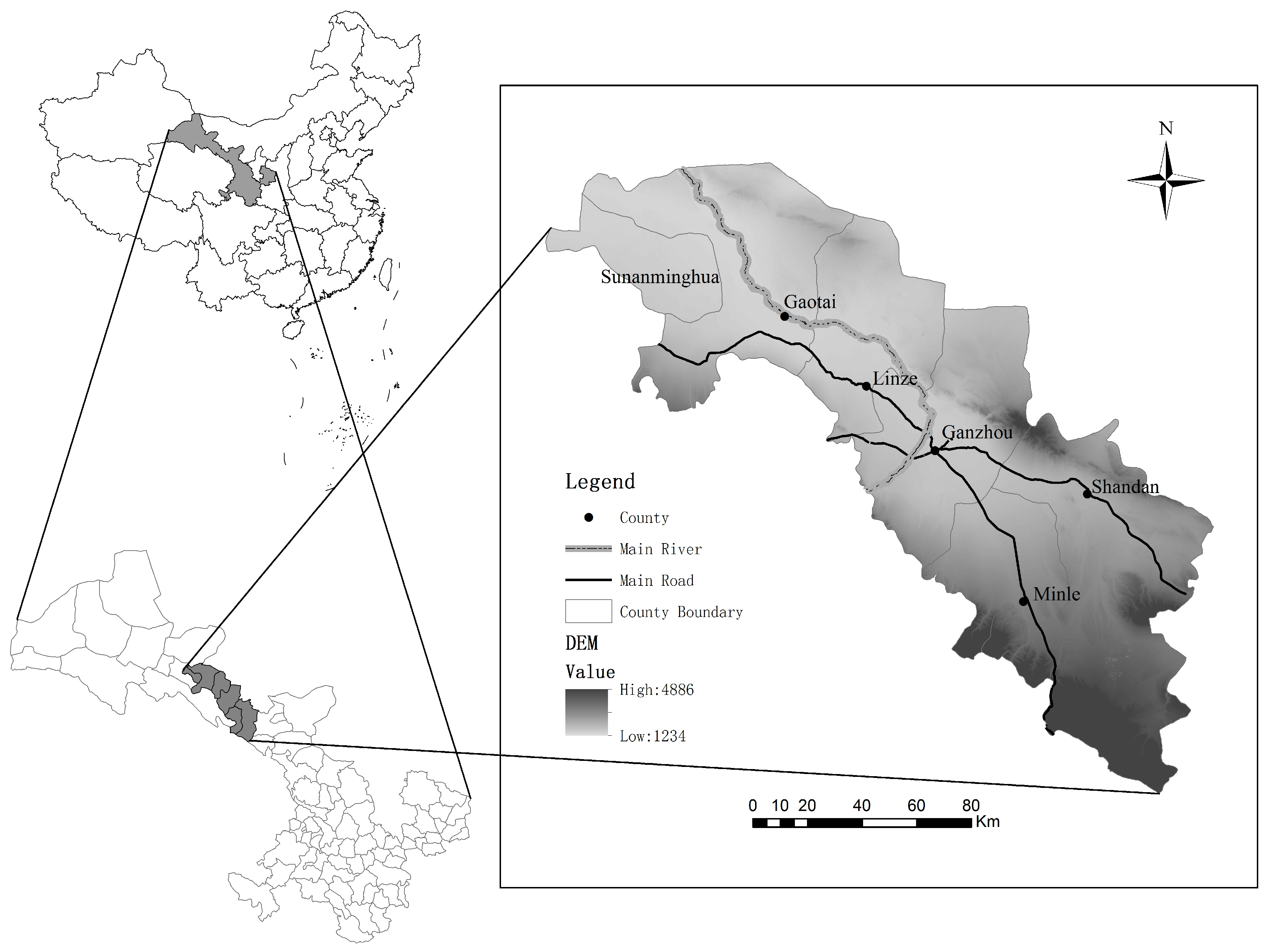
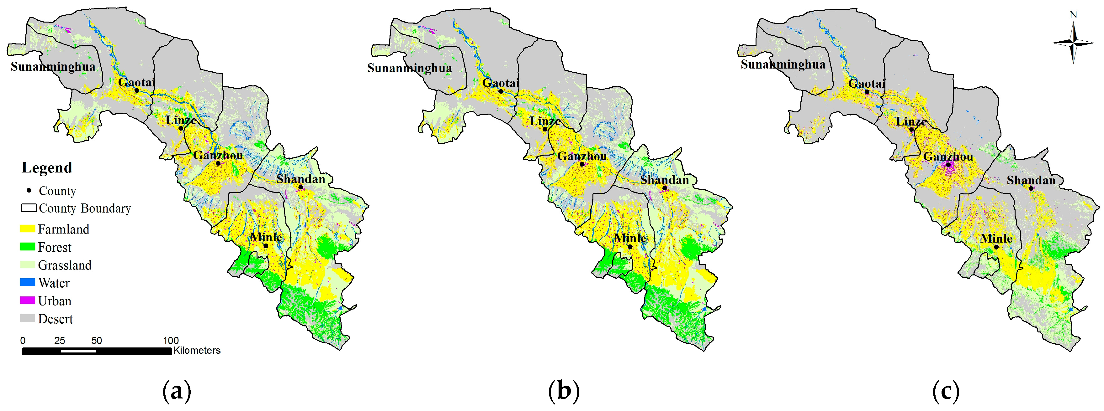
2. Study Area
3. Materials and Methods
3.1. Data Sources
3.2. Risk District Division
3.3. Land Use Ecological Risk Structure
3.3.1. Landscape Disturbance Index (Ei)
3.3.2. Landscape Fragility Index (Fi)
3.3.3. Landscape Ecological Loss Degree (R)
3.3.4. Ecological Risk Index of Land Use (ERI)
3.4. Spatial Statistical Analysis
3.4.1. Spatial Autocorrelation Analysis
3.4.2. Semivariance Analysis
4. Results
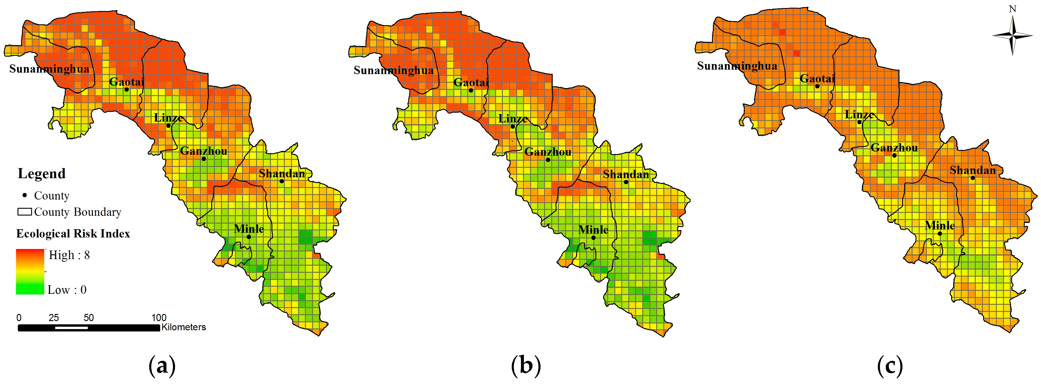
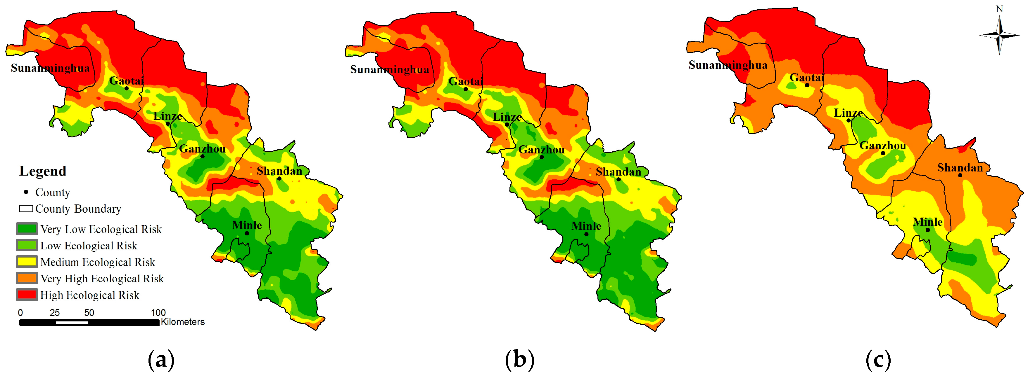
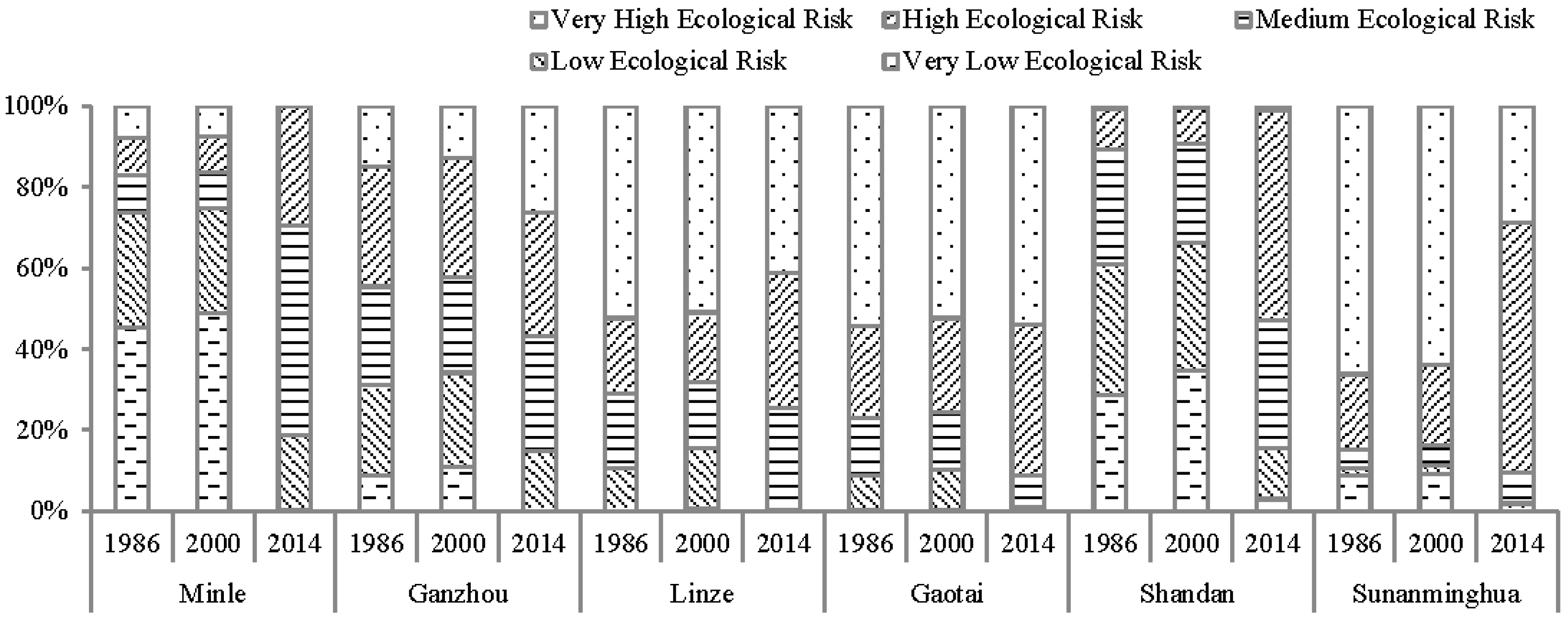
4.1. Temporal and Spatial Dynamic Characteristics of the Ecological Risk Index
4.2. Global Moran’s I of the Ecological Risk Index
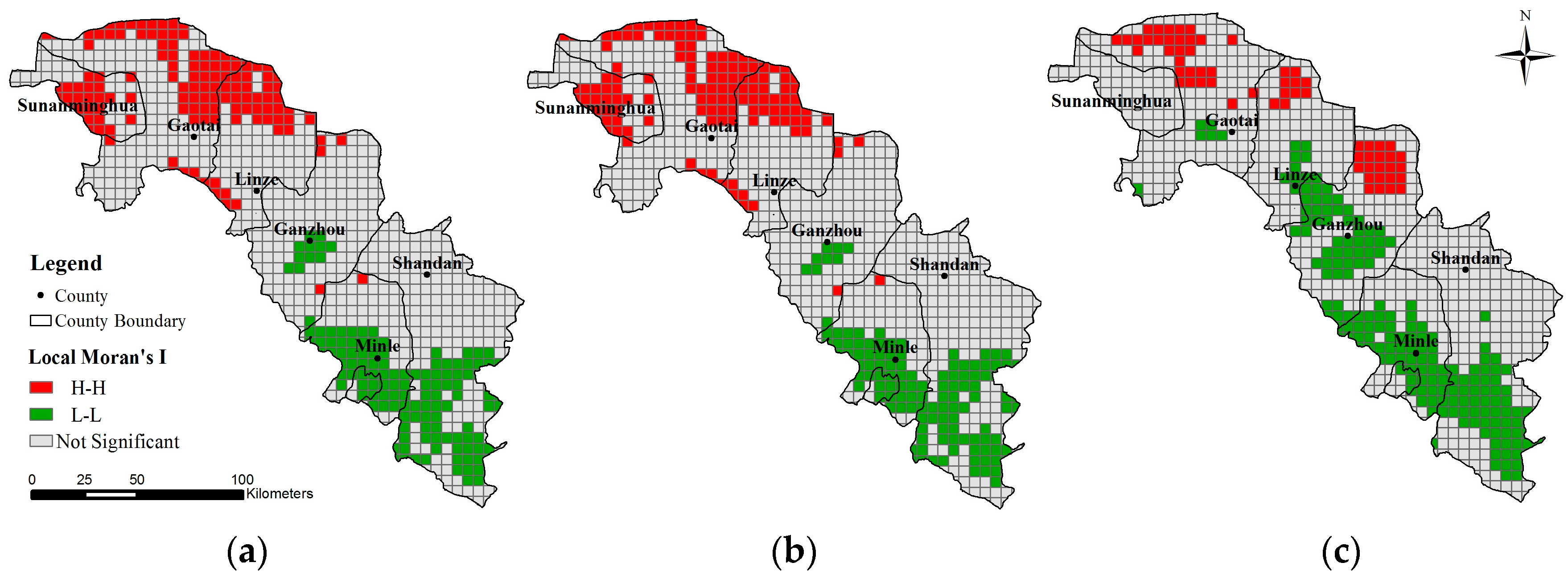
4.3. Local Moran’s I of the Ecological Risk Index
4.4. Spatial Fitting of the Ecological Risk Index
4.5. Spatial Interpolation of the Ecological Risk Index
5. Discussion
6. Conclusions
Acknowledgments
Author Contributions
Conflicts of Interest
References
- Turner, B.L.; Kate, R.W.; Meyer, W.B. The earth as transformed by human action in retrospect. Ann. Assoc. Am. Geogr. 1994, 84, 711–715. [Google Scholar] [CrossRef]
- Moran, E.F. Global land project: Science plan and implementation strategy (IGBP Report No.53/HDP Report No.19.2005). In Proceedings of the Land Open Science Conference, Morelia, Mexico, 2–5 December 2003; IGBP Secretariat: Stockolm, Sweden, 2005. [Google Scholar]
- International Council for Science (ICSU). Future Earth Initial Design (2014–2023); ICSU: Paris, France, 2013. [Google Scholar]
- Zhou, T.; Meng, J.J. Research progress in regional ecological risk assessment methods. Chin. J. Ecol. 2009, 28, 762–767. [Google Scholar]
- Wang, J.W.; Meng, J.J. Ecological risk assessment and management of floods and droughts in the Li River Basin. Trop. Geol. 2014, 34, 366–373. [Google Scholar]
- Tom, B. Ecological risk assessment and quantitative consequence analysis. Hum. Ecol. Risk Assess. 2006, 12, 51–65. [Google Scholar]
- Xiao, D.N.; Bu, R.C.; Li, X.Z. Spatial ecology and landscape heterogeneity. Acta Ecol. Sin. 1997, 17, 453–461. [Google Scholar]
- Zang, S.Y.; Liang, X.; Zhang, S.C. GIS-based analysis of ecological risk on land-use in Daqing City. J. Nat. Disaster. 2005, 14, 141–145. [Google Scholar]
- Xie, H.L. Regional eco-risk analysis of based on landscape structure and spatial statistics. Acta Ecol. Sin. 2008, 28, 5020–5026. [Google Scholar]
- Sun, H.B.; Yang, G.S.; Su, W.Z.; Zhu, T.M.; Wan, R.R. Ecological risk assessment. Acta Ecol. Sin. 2010, 30, 5616–5625. [Google Scholar]
- Zhang, X.B.; Shi, P.J.; Luo, J.; Liu, H.L.; Wei, W. The ecological risk assessment of arid inland river basin at the landscape scale: A case study on Shiyang River Basin. J. Nat. Res. 2014, 29, 410–419. [Google Scholar]
- Gong, W.F.; Yuan, L.; Dang, Y.F. Study on ecological risk of land use in urbanization watershed based on RS and GIS: A case study of Songhua River watershed in Harbin section. Chin. Agric. Sci. Bull. 2012, 28, 255–261. [Google Scholar]
- Zhang, X.F.; Wang, R.S.; Li, Z.G.; Li, F.; Wu, J.S.; Huang, J.L.; Wu, Y.Y. Comprehensive assessment of urban ecological risks: The case of Huaibei City. Acta Ecol. Sin. 2011, 31, 6204–6214. [Google Scholar]
- Yang, Y.F.; Sun, X.H.; Wang, B.T. Ecological risking assessment in Shandong province based on landuse landscape structure. Bull. Soil Water Conserv. 2010, 30, 231–235. [Google Scholar]
- Liu, X.; Su, W.C.; Wang, Z.; Huang, Y.M.; Deng, J.X. Regional ecological risk assessment of land use in the flooding zone of the Three Gorges Reservoir area based on relative risk model. Acta Sci. Circum. 2012, 32, 248–256. [Google Scholar]
- Meng, X.; Ren, Z.Y.; Zhang, C. Study on land use change and ecological risk in Xianyang City. Arid Zone Res. 2012, 29, 137–142. [Google Scholar]
- Bayliss, P.; van Dam, R.A.; Bartolo, R.E. Quantitative ecological risk assessment of the Magela Creek Floodplain in Kakadu National Park, Australia: Comparing point source risks from the ranger uranium mine to diffuse landscape-scale risks. Hum. Ecol. Risk Assess. 2012, 18, 115–151. [Google Scholar] [CrossRef]
- Wang, W.Q.; Li, T.H. Temporal and spatial variation of ecological risk analysis in Yunnan Province based on land use spatial structure. Acta Sci. Nat. Univ. Pek. 2014, 50, 355–360. [Google Scholar]
- Dale, V.H.; Valone, T.J. Ecological principles and guidelines for managing the use of land. Ecol. Appl. 2000, 10, 639–670. [Google Scholar] [CrossRef]
- Xie, H.L. Spatial characteristic analysis of land use eco-risk based on landscape structure: A case study in the Xingguo County, Jiangxi Province. Chin. Environ. Sci. 2011, 31, 688–695. [Google Scholar]
- Wu, J.G. Landscape Ecology-Pattern, Process, Scale and Class, 2nd ed.; Higher Education Press: Beijing, China, 2007. [Google Scholar]
- Liu, J.Y.; Liu, M.L.; Zhuang, D.F. Study on spatial pattern of land-use change in China during 1995–2000. Sci. China 2003, 46, 373–384. [Google Scholar]
- USGS. Science for a changing world. Available online: http://earthexplorer.usgs.gov/ (accessed on 2 June 2016).
- Heihe Planning Data Management Center. Reservoir Data Set of Heihe River Basin; China Cold and Arid Regions Environmental and Engineering Research Institute: Lanzhou, China, 2011. [Google Scholar]
- WestDC. Available online: http://westdc.westgis.ac.cn (accessed on 2 June 2016). (In Chinese)
- Yaacobi, G.; Ziv, Y.; Michael, L. Effects of interactive scale-dependent variables on beetle diversity patterns in a semi-arid agricultural landscape. Landsc. Ecol. 2007, 22, 687–703. [Google Scholar] [CrossRef]
- Qiu, Y.; Yang, L.; Wang, J.; Zhang, Y.; Meng, Q.H.; Zhang, X.G. Grain effect of landscape pattern indices in a gully catchment of Loess Plateau. Chin. J. Appl. Ecol. 2010, 21, 1159–1166. [Google Scholar]
- Shen, W.J.; Wu, J.G.; Lin, Y.B.; Ren, H.; Li, Q.F. Effects of changing grain size on landscape pattern analysis. Acta Ecol. Sin. 2003, 23, 2506–2519. [Google Scholar]
- Li, X.H.; Zhang, J.Y. Analysis on regional landscape ecological risk based on GIS: A case study along the Lower Reaches of the Weihe River. Arid Zone Res. 2008, 25, 899–903. [Google Scholar]
- Jing, Y.P.; Zhang, S.W.; Li, Y. Ecological risk analysis of rural-urban ecotone based on landscape structure. Chin. J. Ecol. 2008, 27, 229–234. [Google Scholar]
- Hu, H.B.; Liu, H.Y.; Hao, J.F. The urbanization effects on watershed landscape structure and their ecological risk assessment. Acta Ecol. Sin. 2011, 31, 3432–3440. [Google Scholar]
- Xu, X.G.; Lin, H.P.; Fu, Z.Y.; Bu, R.C. Regional ecological risk assessment of wetland in the Huanghe River Delta. Acta Sci. Nat. Univ. Pek. 2001, 37, 111–120. [Google Scholar]
- Zeng, H.; Liu, G.J. Analysis of regional ecological risk on landscape structure. Chin. Environ. Sci. 1999, 19, 454–457. [Google Scholar]
- Chen, P.; Pan, X.L. Ecological risk analysis of regional landscape in inland river watershed of arid area: A case study of Sangong River Basin in Fukang. Chin. J. Ecol. 2003, 22, 116–120. [Google Scholar]
- Liu, M.; Zhao, C.W.; Shi, M.H. Spatial autocorrelation analysis of multi-scale land use change at mountainous areas in Guizhou province. Trans. Chin. Soc. Agric. Eng. 2012, 28, 239–246. [Google Scholar]
- Li, X.R.; Li, Y.B.; Han, F.F. Ecological risk assessment of ecological barrier belt in three Gorges Reservoir Areas based on land use. Bull. Soil Water Conserv. 2015, 35, 188–194. [Google Scholar]
- Wang, Z.Q. Statistics and Its Application in Ecology; Science Press: Beijing, China, 1999. [Google Scholar]
- Liu, A.L.; Wang, P.F.; Ding, Y.Y. Introduction to Statistics; Science Press: Beijing, China, 2012. [Google Scholar]
- Meng, J.J. Integrated Physical Geography, 2nd ed.; Peking University Press: Beijing, China, 2011. [Google Scholar]
- Tang, G.A.; Yang, X. ArcGIS Geographic Information System Spatial Analysis Experiment Course; Science Press: Beijing, China, 2006. [Google Scholar]
- Pan, J.H.; Liu, X. Landscape ecological risk assessment and landscape security pattern optimization in Shule River Basin. Chin. J. Ecol. 2016, 35, 791–799. [Google Scholar]
- Sun, X.L.; Fang, C.L. Model and application of ecological risk appraisal in the course of urbanization in arid area. Arid Land Geol. 2006, 29, 668–674. [Google Scholar]


| Grain/m | Moran’s I | ||
|---|---|---|---|
| 1986 | 2000 | 2014 | |
| 5 km | 0.82 | 0.82 | 0.77 |
| 20 km | 0.67 | 0.67 | 0.62 |
| 35 km | 0.58 | 0.58 | 0.49 |
| 50 km | 0.52 | 0.52 | 0.40 |
| 65 km | 0.48 | 0.48 | 0.34 |
| 80 km | 0.45 | 0.44 | 0.31 |
| 95 km | 0.42 | 0.42 | 0.29 |
| 110 km | 0.40 | 0.40 | 0.27 |
| 125 km | 0.38 | 0.38 | 0.26 |
| 140 km | 0.36 | 0.36 | 0.25 |
| Year | Index | Circular | Spherical | Exponential | Gaussian |
|---|---|---|---|---|---|
| 1986 | Mean Standardized | 0.0095 | 0.0108 | 0.0131 | 0.0014 |
| Root Mean Square | 0.7065 | 0.6961 | 0.6197 | 0.7840 | |
| Average Mean Error | 0.8481 | 0.8346 | 0.7062 | 0.9543 | |
| Root-Mean-Square Standardized | 0.8315 | 0.8325 | 0.8749 | 0.8205 | |
| 2000 | Mean Standardized | 0.0100 | 0.0112 | 0.0132 | 0.0024 |
| Root Mean Square | 0.7244 | 0.7139 | 0.6359 | 0.8022 | |
| Average Mean Error | 0.8790 | 0.8656 | 0.7354 | 0.9846 | |
| Root-Mean-Square Standardized | 0.8226 | 0.8231 | 0.8621 | 0.8137 | |
| 2014 | Mean Standardized | 0.0001 | 0.0004 | −0.0014 | 0.0031 |
| Root Mean Square | 0.4846 | 0.4768 | 0.4103 | 0.4905 | |
| Average Mean Error | 0.7040 | 0.6889 | 0.5752 | 0.6651 | |
| Root-Mean-Square Standardized | 0.6889 | 0.6927 | 0.7128 | 0.7387 |
| Year | Sill | Range | Nugget | Partial Sill | Nugget/Sill |
|---|---|---|---|---|---|
| 1986 | 1.0498 | 171.0805 | 0.1073 | 0.9425 | 10.22% |
| 2000 | 1.0488 | 171.0805 | 0.1133 | 0.9355 | 10.80% |
| 2014 | 0.9685 | 84.3180 | 0.1951 | 0.7733 | 20.15% |
| Farmland | Forest | Grassland | Water | Urban | Desert | Sum | ||
|---|---|---|---|---|---|---|---|---|
| 1986–2000 | Farmland | 3475.62 | 0.00 | 37.17 | 0.84 | 14.38 | 0.37 | 3528.40 |
| Forest | 7.73 | 1213.13 | 14.35 | 0.06 | 0.00 | 2.77 | 1238.05 | |
| Grassland | 202.80 | 5.40 | 4509.97 | 2.07 | 0.68 | 13.33 | 4734.25 | |
| Water | 39.79 | 0.00 | 0.11 | 506.85 | 0.03 | 0.20 | 546.98 | |
| Urban | 0.00 | 0.00 | 0.00 | 0.00 | 306.03 | 0.00 | 306.03 | |
| Desert | 22.28 | 1.03 | 1.30 | 1.03 | 0.26 | 9196.84 | 9222.74 | |
| Sum | 3748.23 | 1219.6 | 4562.90 | 510.85 | 321.38 | 9213.52 | 19,576.42 | |
| 2000–2014 | Farmland | 2652.45 | 118.05 | 249.24 | 14.12 | 332.10 | 382.15 | 3748.11 |
| Forest | 41.59 | 317.60 | 565.51 | 1.23 | 10.78 | 282.60 | 1219.31 | |
| Grassland | 281.42 | 291.71 | 1122.30 | 16.18 | 43.76 | 2806.58 | 4561.95 | |
| Water | 36.47 | 28.06 | 64.75 | 107.08 | 9.51 | 264.89 | 510.76 | |
| Urban | 87.13 | 2.91 | 16.53 | 3.68 | 155.08 | 56.04 | 321.36 | |
| Desert | 257.48 | 37.23 | 231.6 | 48.11 | 86.12 | 8552.02 | 9212.56 | |
| Sum | 3356.53 | 795.56 | 2249.93 | 190.40 | 637.35 | 12,344.27 | 19,574.1 | |
| Time | Land Use Type | NP | Pi | Ji | Ni | Ci | Si | DOi |
|---|---|---|---|---|---|---|---|---|
| 2000 | Farmland | 840 | 1.4228 | 99.7661 | 0.0334 | 0.0022 | 0.0541 | 0.2741 |
| Forest | 434 | 1.4310 | 99.4695 | 0.0380 | 0.0036 | 0.1195 | 0.1627 | |
| Grassland | 1485 | 1.4179 | 99.5555 | 0.0351 | 0.0033 | 0.0591 | 0.4242 | |
| Water | 218 | 1.7091 | 99.1523 | 0.0833 | 0.0043 | 0.2022 | 0.1564 | |
| Urban | 2775 | 1.3584 | 93.6813 | 0.1182 | 0.0863 | 1.1467 | 0.2872 | |
| Desert | 356 | 1.4432 | 99.9152 | 0.0144 | 0.0004 | 0.0143 | 0.4472 | |
| 2014 | Farmland | 4523 | 1.2674 | 99.7472 | 0.0434 | 0.0135 | 0.1402 | 0.2527 |
| Forest | 8101 | 1.3004 | 98.8745 | 0.0875 | 0.1018 | 0.7915 | 0.2261 | |
| Grassland | 13,790 | 1.2708 | 99.4858 | 0.0679 | 0.0613 | 0.3651 | 0.3064 | |
| Water | 2378 | 1.2787 | 98.5747 | 0.0997 | 0.1248 | 1.7915 | 0.1949 | |
| Urban | 13,871 | 1.3049 | 97.4653 | 0.1456 | 0.2176 | 1.2932 | 0.3486 | |
| Desert | 9643 | 1.1938 | 99.9372 | 0.0253 | 0.0078 | 0.0556 | 0.6228 |
© 2016 by the authors; licensee MDPI, Basel, Switzerland. This article is an open access article distributed under the terms and conditions of the Creative Commons Attribution (CC-BY) license (http://creativecommons.org/licenses/by/4.0/).
Share and Cite
Fan, J.; Wang, Y.; Zhou, Z.; You, N.; Meng, J. Dynamic Ecological Risk Assessment and Management of Land Use in the Middle Reaches of the Heihe River Based on Landscape Patterns and Spatial Statistics. Sustainability 2016, 8, 536. https://doi.org/10.3390/su8060536
Fan J, Wang Y, Zhou Z, You N, Meng J. Dynamic Ecological Risk Assessment and Management of Land Use in the Middle Reaches of the Heihe River Based on Landscape Patterns and Spatial Statistics. Sustainability. 2016; 8(6):536. https://doi.org/10.3390/su8060536
Chicago/Turabian StyleFan, Jiahui, Ya Wang, Zhen Zhou, Nanshan You, and Jijun Meng. 2016. "Dynamic Ecological Risk Assessment and Management of Land Use in the Middle Reaches of the Heihe River Based on Landscape Patterns and Spatial Statistics" Sustainability 8, no. 6: 536. https://doi.org/10.3390/su8060536
APA StyleFan, J., Wang, Y., Zhou, Z., You, N., & Meng, J. (2016). Dynamic Ecological Risk Assessment and Management of Land Use in the Middle Reaches of the Heihe River Based on Landscape Patterns and Spatial Statistics. Sustainability, 8(6), 536. https://doi.org/10.3390/su8060536