Article

Estimating the Contribution of Industry Structure Adjustment to the Carbon Intensity Target: A Case of Guangdong

School of Management, Jinan University, Guangdong 510632, China
*
Author to whom correspondence should be addressed.
Sustainability 2016, 8(4), 355; https://doi.org/10.3390/su8040355
Submission received: 26 January 2016 / Revised: 17 March 2016 / Accepted: 6 April 2016 / Published: 12 April 2016

Abstract

:
Industry structure adjustment is an effective measure to achieve the carbon intensity target of Guangdong Province. Accurately evaluating the contribution of industry structure adjustment to the carbon intensity target is helpful for the government to implement more flexible and effective policies and measures for CO2 emissions reduction. In this paper, we attempt to evaluate the contribution of industry structure adjustment to the carbon intensity target. Firstly, we predict the gross domestic product (GDP) with scenario forecasting, industry structure with the Markov chain model, CO2 emissions with a novel correlation mode based on least squares support vector machine, and then we assess the contribution of industry structure adjustment to the carbon intensity target of Guangdong during the period of 2011–2015 under nine scenarios. The obtained results show, in the ideal scenario, that the economy will grow at a high speed and the industry structure will be significantly adjusted, and thus the carbon intensity in 2015 will decrease by 25.53% compared to that in 2010, which will make a 130.94% contribution to the carbon intensity target. Meanwhile, in the conservative scenario, the economy will grow at a low speed and the industry structure will be slightly adjusted, and thus the carbon intensity in 2015 will decrease by 23.89% compared to that in 2010, which will make a 122.50% contribution to the carbon intensity target.

1. Introduction

Climate change is one of the most serious challenges for global sustainable development in the 21st century. To address the global climate change, the Chinese government announced that carbon intensity, defined by the comparison between CO2 emissions and gross domestic product (GDP), should be reduced by 40%–45% from 2005 to 2020. For the purpose of achieving this target, China’s state council issued the greenhouse gas emissions control scheme during the 12th five-year plan (2011–2015) (China made the first “five-year plan (1953–1957)” in 1953; so far, China has published 12 five-year plans, and the 13th five-year plan (2016–2020) will be developed in 2016) to allocate the CO2 emissions reduction tasks for every province in 2012, in which Guangdong’s carbon intensity should decrease 19.5% from 2010 to 2015. Industry structure adjustment, which is trying to coordinate the proportions of primary, secondary and tertiary industries, naturally becomes an effective way for achieving the carbon intensity target [1], because it can effectively reduce the carbon intensity. Through industry structure adjustment, realizing the carbon intensity target requires solving two questions: how much will industry structure adjustment reduce the carbon intensity, and how much will industry structure adjustment realize the carbon intensity target?
Located in southern China, Guangdong Province is adjacent to the special administrative regions of Hong Kong and Macao. In 2014, Guangdong’s GDP reached 6.78 billion Yuan at the current price, accounting for over 10% of that of the whole country. At that time, it had ranked first in terms of economic performance for over 20 successive years. The permanent population of Guangdong was 107.24 million in 2014, ranking first in China. During 1990–2014, Guangdong’s energy consumption increased rapidly, from 36.90 to 256.36 million tons standard coal, implying a mean annual increase of 8.41%. Furthermore, such a large increase in energy consumption will certainly cause a large increase in CO2 emissions. Thus, there will be tremendous pressure on Guangdong to realize this goal during the period of the 12th five-year plan (2011–2015).
During the past few years, some scholars have developed related research on the realization of the carbon intensity target from different angles using various methods [2,3,4,5,6,7,8,9,10,11,12,13,14,15]. These studies show that industry structure adjustment is one of the effective measures for decreasing carbon intensity, which can provide some important references for making out energy conservation and emission reduction policies. However, the existing research mainly focused on the national level, and ignored the larger differences among resource endowments and industry foundations of various provinces [16]. Their obtained conclusions and relevant policies cannot have a good credibility and feasibility; thus, it is difficult for various provinces to guide their practices. Moreover, the existing studies mainly used the input-output method and structure decomposition method. The former needs to use the input-output table data, which usually applies to the national level rather than provincial level for the lack of enough data, while the latter is usually used to explore the inner mechanism of carbon intensity changes, and is seldom used to estimate the contribution of industry structure adjustment to the carbon intensity target. So far, rare literature has been found in terms of evaluating the contribution of industry structure adjustment to the carbon intensity target of Guangdong.
In order to fill this gap, this study mainly contributes to and aims at evaluating the contribution of industry structure adjustment to the carbon intensity target by an integrated use of multidisciplinary approaches. Firstly, we predict GDP with scenario forecasting, industry structure with the Markov chain model, CO2 emissions with a novel correlation model based on least squares support vector machines (LSSVM), and then we assess the contribution of industry structure adjustment to the carbon intensity target of Guangdong in 2015 under nine scenarios. The obtained results show, in the ideal scenario, that the economy will grow at a high speed and the industry structure will be significantly adjusted, and thus the carbon intensity will decrease by 25.53% from 2010 to 2015, which will make a 130.94% contribution to the carbon intensity target. Meanwhile, in the conservative scenario, the economy will grow at a low speed and the industry structure will be slightly adjusted, and thus the carbon intensity will decrease by 23.89% from 2010 to 2015, which will make a 122.50% contribution to the carbon intensity target. This study can help answer the above two questions, and providing theoretical support for decision-making for the related governments.

2. Methods and Data

As a relative index, carbon intensity is defined as: carbon intensity = CO2 emission/GDP. Thus, we will forecast CO2 emissions and GDP respectively. Firstly, we will set three scenarios to predict the GDP. Secondly, we will employ the Markov chain model to predict the industry structure. Thirdly, we will calculate and forecast CO2 emissions with a novel correlation model based on LSSVM under various industry structure scenarios. Finally, we will evaluate the contribution of industry structure adjustment to the carbon intensity target.

2.1. GDP Forecasting

Using scenario prediction, GDP is forecasted by:
G D P 2014 + i = G D P 2014 × ( 1 + r ) i , i = 1 , 2 ,
where r is the average annual growth rate of the GDP.

2.2. Industry Structure Prediction with the Markov Chain Model

In this study, we use the Markov chain model [17] to predict the industry structure by 2015. The state vector of the industry structure at year n is defined as S ( n ) : S ( n ) = { s a ( n ) , s b ( n ) , s c ( n ) } , where s a ( n ) , s b ( n ) , s c ( n ) are the respective proportions of the primary, secondary and tertiary industries.
The one-step transition probability matrix of industry structure from n to n + 1 is defined as:
[ M a a ( n )    M a b ( n )    M a c ( n ) M b a ( n )    M b b ( n )    M b c ( n ) M c a ( n )    M c b ( n )    M c c ( n ) ]
where the elements in the leading diagonals of the transition probability matrix are, respectively, the probabilities of three industries for maintaining their original structures. Except the leading elements, other elements are the transition probabilities; the row elements show the probability of one industry transferring to the other industries. The column element represents the probability of specific gravity of other industries transferring to one certain industry; the sum of the transition probability in each row is 1.
For convenience, the elements in the leading diagonals of the transition probability matrix are called reserved probability elements. Except the reserved probability elements, other elements in the rows are called the transition probability elements. Elements in the column, except the reserved probability elements, are named after absorptive elements.
We use the Markov chain model to predicate the industry structure as follows:
(1) Calculate the reserved probability element. For the industry structure, if the proportion of one industry increases from the nth year to the n+1th year, the reserved probability of this industry in the transition probability matrix is 1. Otherwise, the reserved probability is the ratio of the proportion of the n+1th year to that of the nth year. Taking coal as an example:
S a ( n + 1 ) S a ( n ) M a a ( n ) = 1
S a ( n + 1 ) < S a ( n ) M a a ( n ) = S a ( n + 1 ) / S a ( n )
(2) Compute the transition probability elements in the row in which an element with the reserved probability is 1. The value of the reserved probability elements in a certain row is 1, which shows that the proportion of one certain energy represented by this row is unchanged or increases, and thus the certain energy cannot transfer to the other energies. Besides, the sum of the transition probability in each row is 1. Therefore, each transition probability element in this row is 0. Taking primary industry as an example:
M a a ( n ) = 1 { M a b ( n ) = 0 ; M a c ( n ) = 0 }
(3) Calculate the absorptive probability elements in the column where the reserved probability is less than 1. The reserved probability element in a certain column is less than 1, which implies that the proportion of the certain industry represented by this column decreases, and other industries cannot transfer to this industry. Therefore, each absorptive probability element in this column is 0. Taking primary industry as an instance:
M a a ( n ) < 1 { M b a ( n ) = 0 ; M c a ( n ) = 0 }
(4) Compute the elements of non-zero transition probability in the row where the reserved probability is less than 1. As for primary industry, taking the scenario where the reserved probability is less than 1 as an example:
M a a ( n ) < 1 M a b ( n ) 0 M a c ( n ) 0 } { M a b ( n ) = [ 1 M a a ( n ) ] × [ S b ( n + 1 ) S b ( n ) ] [ S b ( n + 1 ) S b ( n ) ] + [ S c ( n + 1 ) S c ( n ) ] + [ S d ( n + 1 ) S d ( n ) ] M a c ( n ) = [ 1 M a a ( n ) ] × [ S c ( n + 1 ) S c ( n ) ] [ S b ( n + 1 ) S b ( n ) ] + [ S c ( n + 1 ) S c ( n ) ] + [ S d ( n + 1 ) S d ( n ) ]
(5) Repeat the above steps (1)–(4); the transition probability matrixes of the industry structure in each year are, respectively, M ( 1 ) , M ( 2 ) , , M ( n ) , from the initial year to the nth year. The average matrix of the transition probability is achieved as:
M = [ i = 1 n M ( i ) ] 1 / n
(6) Forecast the industry structure in the n+lth year:
S ( n + l ) = S ( n ) M l

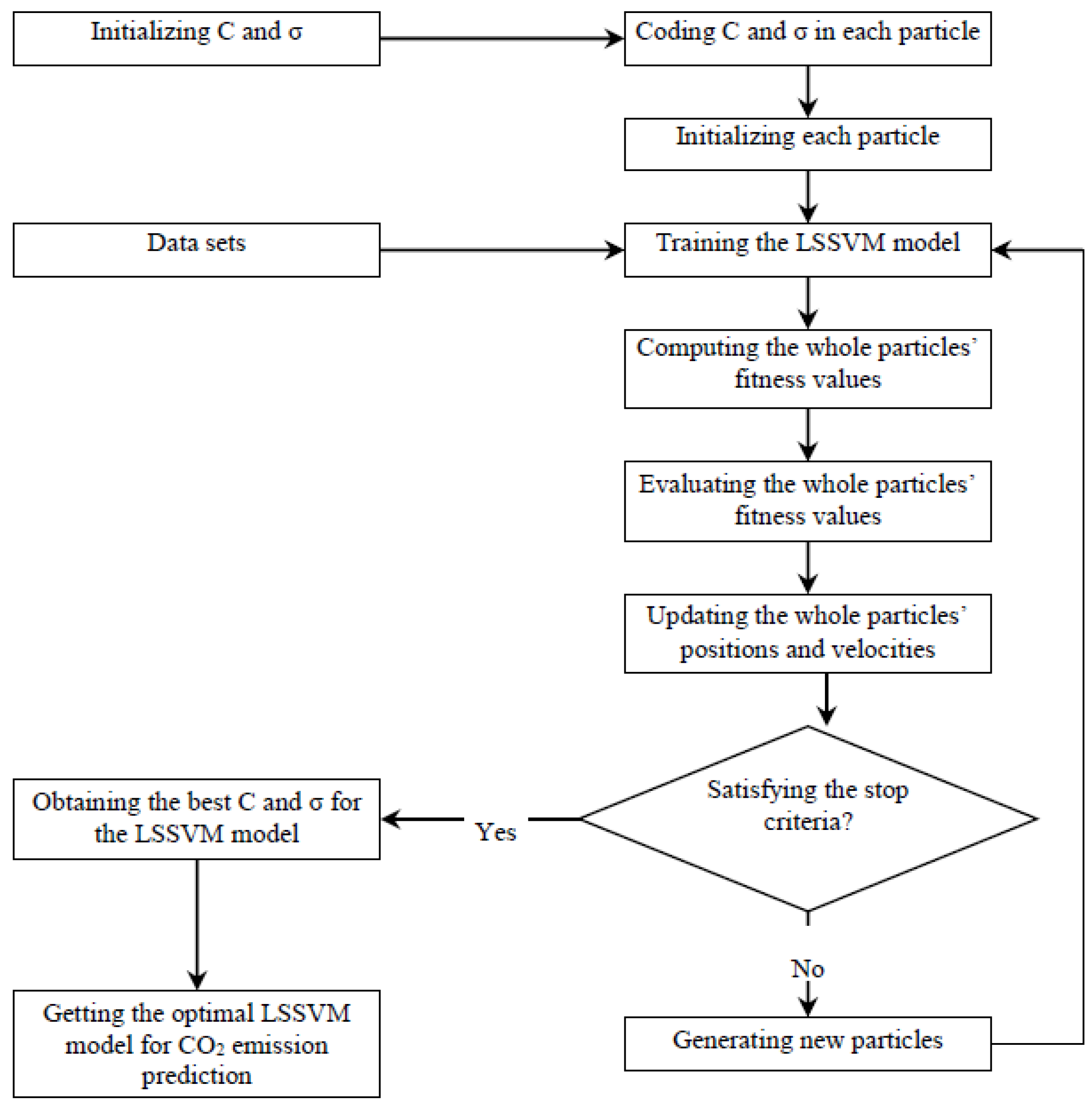
2.3. Estimating CO2 Emissions

Energy consumption is the main source of CO2 emissions, accounting for more than 90% of the total CO2 emissions in China. Inspired by the reference method for estimating CO2 emissions of the International Panel on Climate Change [18], we calculate the CO2 emissions of primary energy consumption as:
C E = i = 1 4 E i × C o e i × 44 12
where CE is the total CO2 emissions, E1, E2, E3 and E4 are consumptions of the coal, petroleum, natural gas and non-fossil energies, respectively; Coe1, Coe2, Coe3 and Coe4, respectively, are carbon emission coefficients of the coal, petroleum, natural gas and non-fossil energies.

2.4. Forecasting CO2 Emissions

Inspired by the method proposed by [19], we set up a new correlation model incorporating industry structure and LSSVM to predict the CO2 emissions under various industry structure scenarios, defined by:
C E = f ( x ) ,   x = ( x 1 , x 2 , x 3 )
where x 1 , x 2 and x 3 are the proportions of the primary, secondary and tertiary industries, respectively, and f ( ) is a nonlinear function determined by the LSSVM model.
As a novel machine learning approach for small-sample data, for a given training set { x i , y i } , i = 1 , 2 , , l with input data x i , and output data y i , LSSVM defines the regression function as [20]:
m i n Q ( ω , b , e ) = 1 2 ω 2 + C 2 i = 1 l e i 2 s . t .      y i = ω T φ ( x i ) + b + e i    i = 1 , 2 , , l
where w is the weight vector, C is the penalty parameter, e i is the approximation error, φ ( ) is the nonlinear mapping function and b is the bias term. The corresponding Lagrange function can be obtained:
L ( w , e , α , b ) = J ( w , e ) i = 1 l α i { w T φ ( x i ) + b + e i y i }
where α i is the Lagrange multiplier. Using the Karush–Kuhn–Tucker (KKT) conditions, the solutions can be obtained by partially differentiating with respect to w , b , e i and α i :
{ L ω = 0 ω = i = 1 l a i φ ( x i ) L b = 0 i = 1 l a i = 0 L e i = 0 a i = C e i L a i = 0 ω T φ ( x i ) + b + e i y i = 0
By eliminating w and e i , the equations can be changed into
[ 0 1 v T 1 v Ω + C 1 I ] [ b a ] = [ 0 y ]
where y = [ y 1 , y 2 , , y l ] T , I v = [ 1 , 1 , , 1 ] T , α = [ α 1 , α 2 , , α l ] T , and the Mercer condition has been applied to matrix Ω with Ω k m = φ ( x k ) T φ ( x k ) , k , m = 1 , 2 , , l . Therefore, the LSSVM for regression can be obtained:
y ( x ) = i = 1 l α i K ( x , x i ) + b
where K ( x , x i ) is the kernel function.
The establishment of a LSSVM model requires two key issues to be addressed [21]. These are, firstly, how does one make an appropriate choice of the kernel function? Secondly, how does one accurately determine the model parameters? In this study, the first issue is solved by using the radial basis kernel function (RBF), K ( x , y ) = exp ( x y 2 / 2 σ 2 ) , to build the LSSVM model. This is because this function generally yields good predictions [22]. For the second issue, particle swarm optimization (PSO), proposed by Kennedy and Eberhart [23], is adopted to find out the best values of C and σ [24].
PSO represents each candidate solution by the state of a particle in a search space. M particles constitute a swarm in a two-dimensional space. Vectors x i = ( x i 1 , x i 2 ) and v i = ( v i 1 , v i 2 ) , respectively, express the position and velocity of particle i. Other vectors p b e s t = ( p i 1 , p i 2 ) and g b e s t = ( g i 1 , g i 2 ) , respectively, express the optimum positions of particle i and all particles at the present stage. The position and velocity of every particle are renewed according to the following formulas:
x i d ( t + 1 ) = { p max , x i d < p max x i d ( t ) + v i d ( t + 1 ) , p max x i d p max p max , x i d > p max
v i d ( t + 1 ) = { v max , v i d < v max w ( t ) v i d ( t ) + c 1 r 1 [ p i d ( t ) x i d ( t ) ] + c 2 r 2 [ p g d ( t ) x i d ( t ) ] , v max v i d v max v max , v i d > v max
where 1 i m , 1 d M , v i d ( t ) denotes the velocity of particle i at iteration t, and x i d ( t ) signifies the position of particle i at iteration t. Also, p i d is the previous optimum position of particle i, p g d is all particles’ greatest position, and w is the inertia weight. The latter is generally set as a function that decreases linearly with time as:
w ( t ) = w max w max w min t max × t
where w max and w min are, respectively, the biggest and smallest inertia weights.
In this study, PSO is introduced to find the optimal LSSVM model parameters ( C and σ ) to enhance search efficiency and prediction accuracy. Figure 1 illustrates the process of LSSVM parameter searching using PSO. In greater detail, the steps unfold as follows:
Step 1: Establish training and testing sets. The data gathered during a certain period are, respectively, separated into a training set employed in building the model, and a test set used for checking the model’s predictive performance.
Step 2: PSO initialization. First, m particles can be randomly produced by coding C and σ with real values. Then, PSO parameters are set as: t max (maximal iterations), p max (maximal position), v max (maximal velocity), w max (maximal inertia weight), w min (minimum inertia weight), c 1 and c 2 (acceleration coefficients), C min (minimum C ) and C max (maximal C ), σ min (minimum σ ) and σ max (maximal σ ). Training begins when t = 0.
Step 3: Choose the root mean square error (RMSE) as each particle’s fitness function:
R M S E = 1 n i = 1 n ( x i x ^ i ) 2
In this formula, n is the amount of training samples, x i is the real value, and x ^ i is the predictive value.
Step 4: Appraise fitness. Compute the fitness values of entire particles using Equation (4). Then, find out p b e s t and g b e s t at the current generation.
Step 5: Renew the positions and velocities of the whole particles using Equations (1)–(3).
Step 6: Check terminal conditions. The search process is terminated when the termination criteria, such as the maximum number of iterations, etc., are satisfied. If fulfilled, output the optimal values. Otherwise, repeat Step 7 iteratively.
Step 7: Let t = t + 1 , and recur to Step 4.

2.5. Evaluating the Contribution of the Carbon Intensity Target

The contribution of the carbon intensity target is defined as:
d = C I R C I T = ( C I 2015 C I 2010 ) / C I 2010 C I T × 100 %
where d is the contribution of the carbon intensity target; CIR is the carbon intensity reduction amplitude; CIT is the carbon intensity reduction target; CI2015 and CI2010 are the carbon intensities in 2015 and in 2010, respectively.
By combining the scenarios of different economic growth and industry structure, various combined scenarios can be formed in total. The value of d in a certain scenario is equal to or greater than 100%, which indicates that the carbon intensity target can be accomplished under this scenario. If not, the value of d is less than 100%, which shows that Guangdong cannot achieve the target.

2.6. Data

Selecting the data from 1990–2014 as the study samples, except for carbon emission coefficients and CO2 emissions, we have obtained all the data from the Guangdong Statistical Yearbook (2015) [25]. GDP data (unit: 100 million Yuan) are adjusted as the constant price in 1978. E is converted into standard coal, with the unit of 10,000 tons of standard coal.
The carbon emission coefficients are the values of those recommended by the State Development and Reform Commission in China, namely Coe1 = 0.7476, Coe2 = 0.5825, Coe3 = 0.4435 and Coe4 = 0, with the unit of t(C)/t. CO2 emissions from 1990 to 2014 in Guangdong estimated by this study are illustrated in Figure 2. It can be observed that CO2 emissions in Guangdong have increased sharply from 84.98 million tons in 1990 to 499.52 million tons in 2011, down to 483.98 million tons in 2012, up to 485.72 million tons in 2013, and down to 481.09 million tons in 2014. At the same time, the carbon intensity in Guangdong has decreased significantly from 13.89 ton/104 RMB Yuan in 1990 to 3.69 ton/104 RMB Yuan in 2014 at the fixed price of 1978.

3. Results and Discussion

3.1. Prediction on GDP of Guangdong in 2015

Although Guangdong clearly stated that the expected average annual growth rate of GDP should be above 8% during 2010–2015, the real one reached 7.58% at the fixed price of 1978 during the period of 2010–2014. The main reasons may be two-fold: one is that the global economic downturn has hit Chinese economic growth, and the other is that China is committed to the industrial structure transformation, which has brought a slower economic growth than ever. Economic growth is expected to fall further by 2015. Thus, we set up three scenarios for economic growth: high-speed with an average annual growth rate of 7.7%, medium-speed with an average annual growth rate of 7.5%, and low-speed with an average annual growth rate of 7.3%. On this basis, the GDP of Guangdong in 2015 will reach 14,057.98 (high-speed scenario), 14,031.87 (medium-speed scenario) and 14,005.77 billion RMB Yuan (low-speed scenario) at the fixed price of 1978.

3.2. Prediction on Industry Structure of Guangdong in 2015

The industry structure data in Guangdong from 2010 to 2014 are used to calculate the transition probability matrix of the Markov chain model. In this way, we can obtain the transition probability matrixes of the energy structure in each step during 2010 to 2014, which can be used to calculate the average transition probability matrix as follows:
M = [ 0.9816 0 0.0184 0 0.9792 0.0208 0 0 1 ]
Then, we can forecast the industry structure in 2015 under the natural evolution: S ( 2015 ) = S ( 2014 + 1 ) = S ( 2014 ) M . Thus, we can obtain the industry structure in 2015: primary industry (4.58%), secondary industry (45.38%) and tertiary industry (50.04%).
The future trend of the industry structure is merely forecasted based on the evolution law of the historical industry structure instead of the adjustment of the national and provincial policies. Here, we define this as the industry structure “minor adjustment” scenario. Thus, we can obtain the industry structure under the “minor adjustment” scenario: primary industry (4.58%), secondary industry (45.38%) and tertiary industry (50.04%).
Taking this as an important strategic task, Guangdong has implemented an innovation-driven development strategy to promote economic structural adjustment and industrial transformation and upgrading since 2013. It is supposed that on the basis of minor adjustment, the proportion of tertiary industry will increase 0.5% in 2015, which will obtained by reducing the proportion of secondary industry. In this study, this scenario is called “medium adjustment”. Under “medium adjustment”, Guangdong’s industry structure will be: primary industry (4.58%), secondary industry (44.88%) and tertiary industry (50.54%) by 2015.
Guangdong has not set up a target for primary industry by 2015. However, the proportion of primary industry in Guangdong has steadily decreased during recent years, which is in accordance with the industry structure evolution law of developed countries, namely economic development will inevitably result in the decrease of the proportion of primary industry. In fact, the proportion of tertiary industry rises at the cost of the synergistic decreases of the proportions of primary industry and secondary industry, rather than secondary industry alone. The continued increase in tertiary industry can alleviate CO2 emissions to some extent. To achieve the CO2 emissions reduction target of Guangdong, it appears necessary to increase the proportion of tertiary industry as soon as possible. Suppose that the proportion of primary industry will decrease from 5.03% in 2010 to 4.5% in 2015, and that the proportional decrease will be achieved by increasing the proportion of tertiary industry. Thus, the industry structure with planning restrictions and primary industry target restriction is predicted. In this study, this scenario is called “substantial adjustment”. Accordingly, Guangdong’s industry structure under “substantial adjustment” by 2015 is: primary industry (4.50%), secondary industry (44.88%) and tertiary industry (50.62%).

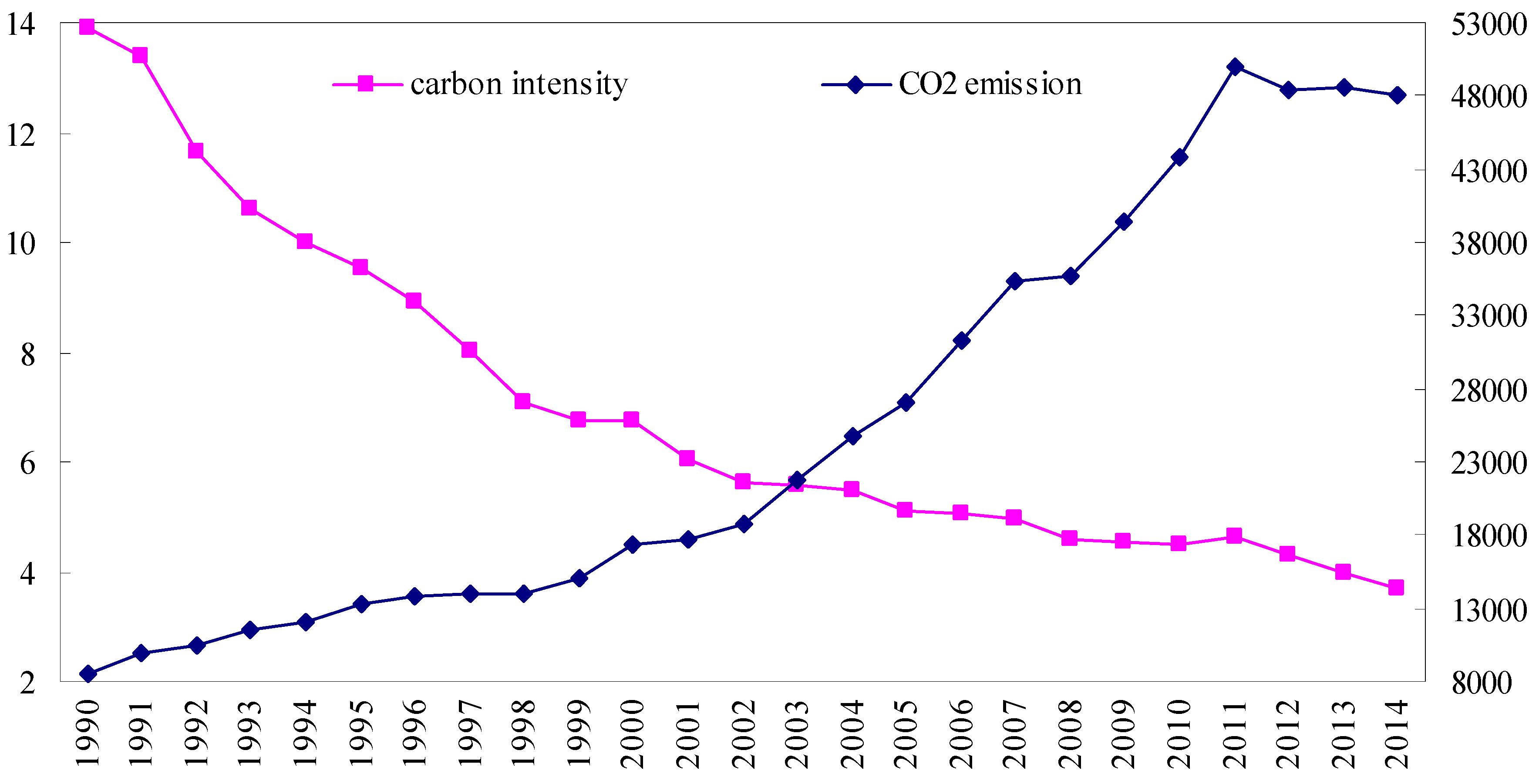
3.3. Prediction on CO2 Emissions of Guangdong in 2015

For the data from 1990 to 2014 in Guangdong, we use the five-fold cross-validation method [22] to train the LSSVM model, and we obtain the best values of the model parameters: C = 359.8661 ,   σ = 4.1248 . Once the LSSVM model has been trained, the future industry structure is input into the trained LSSVM model so as to obtain the CO2 emissions in the corresponding year. Thus, we input the industry structures under the “minor adjustment”, “medium adjustment” and “substantial adjustment” scenarios for 2015, and obtain successively the forecasted CO2 emissions of 478.82, 473.86 and 470.21 million tons for 2015.

3.4. Prediction on Carbon Intensity of Guangdong in 2015

Guangdong’s CO2 emissions were 437.69 million tons and the constant-price GDP was 974.44 billion RMB Yuan in 2010. Thus, the carbon intensity was 4.4917 ton/104 RMB Yuan in 2010. Table 1 lists the predicted values of Guangdong’s carbon intensity under different scenarios in 2015 with the unit of ton/104 RMB Yuan. Taking the high-speed economic growth as an example, under the “minor adjustment” scenario, the carbon intensity will reduce from 4.4917 ton/104 RMB Yuan in 2010 to 3.4061 ton/104 RMB Yuan, decreased by 24.17%. Under the “medium adjustment” scenario, the carbon intensity will reduce from 4.4917 ton/104 RMB Yuan in 2010 to 3.3708 ton/104 RMB Yuan, decreased by 24.95%. Under the “substantial adjustment” scenario, the carbon intensity will reduce from 4.4917 ton/104 RMB Yuan in 2010 to 3.3448 ton/104 RMB Yuan, decreased by 25.53%.

3.5. Prediction on CO2 Emissions of Guangdong in 2015

According to “China’s 12th five-year control scheme for greenhouse gas emissions”, in 2015, Guangdong’s carbon intensity should be 19.5% lower than that in 2010. By combining the above scenarios of economic growth with industry structure adjustment, nine combined scenarios are formed in total. We calculate the amplitude of the carbon intensity reduction, as well as the potential of the industry structure adjustment to reach the carbon intensity target under each combined scenario compared with 2010. The specific results are shown in Table 2 (in %).
It can be found that, for a given level of economic growth, the larger the industry structure adjustment, the larger its “reduction amplitude” and “contribution” to achieving the carbon intensity target. For a given industry structure adjustment, the higher the economic growth, the larger its “reduction amplitude” and “contribution” to realizing the carbon intensity target. Under all scenarios, each of the contributions to the carbon intensity target will exceed 100%, which means a 19.5% decline in carbon intensity can be realized by industry structure adjustment. We can cautiously conclude that it appears to be feasible for Guangdong’s government to reach its carbon intensity goal by 2015.

4. Conclusions

Using the data from 1990–2014 in Guangdong as well as the integrated use of multidisciplinary approaches, including the Markov chain model, least squares support vector machine and scenario prediction, we calculate Guangdong’s GDP, industry structure, CO2 emissions, and carbon intensity by 2015. Moreover, we evaluate the contribution of industry structure adjustment to the “12th five-year” carbon intensity target under nine combined scenarios. From this, we make the following conclusions:
(i)
Industry structure adjustment is an effective measure for driving the reduction of carbon intensity. For a given level of economic growth, the larger the industry structure adjustment, the larger the “reduction amplitude” of the carbon intensity. For a given industry structure adjustment, the higher the economic growth, the larger the “reduction amplitude” of the carbon intensity.
(ii)
Under the ideal scenario (i.e., “high-speed economic growth” and “substantial industry structure adjustment”), industry structure adjustment contributes most to the realization of the carbon intensity goal, with a contribution of 130.94%. Carbon intensity would be reduced by 25.53% in 2015 as compared to 2010. Under the conservative scenario (i.e., “low-speed economic growth” and “minor industry structure adjustment”), the contribution of industry structure adjustment to meeting the carbon intensity goal will reach 122.50%. At the same time, the carbon intensity in 2015 will decrease by 23.89% as compared to 2010.
(iii)
The reduction by 19.5% of the carbon intensity goal can be achieved under all the combined scenarios through industry structure adjustment. Thus, it can be concluded that the set target appears scientific and reasonable for Guangdong’s government to reach its carbon intensity goal by 2015.
(iv)
Although the obtained results show that the goal of reducing 19.5% of Guangdong’s carbon intensity can be achieved, there are some limitations and uncertainties. In this paper, we have not taken into account the adoption and use of novel low carbon policies, which will change over time. How to capture them is the focus of one of our next works.

Acknowledgments

We thank two anonymous referees for their valuable comments. Our heartfelt thanks should also be given to the National Natural Science Foundation of China (NSFC) (71201010, 71303174 and 71473180), National Philosophy and Social Science Foundation of China (14AZD068, 15ZDA054), Natural Science Foundation for Distinguished Young Talents of Guangdong (2014A030306031), Soft Science Foundation of Guangdong (2014A070703062), Social Science Foundation of Guangdong (GD14XYJ21), Distinguished Young Teachers of Guangdong ([2014]145), High-level Personnel Project of Guangdong ([2013]246), Guangdong key base of humanities and social science: Enterprise Development Research Institute and Institute of Resource, Environment and Sustainable Development Research, and Guangzhou key base of humanities and social science: Centre for Low Carbon Economic Research for funding supports.

Author Contributions

This work was designed, analyzed, and written by the first author. The data were gathered and disposed by both the authors. The LSSVM modeling was built by the second author.

Conflicts of Interest

The authors declare no conflict of interest.

References

  1. Xiang, N.; Xu, F.; Sha, J.H. Simulation Analysis of China’s Energy and Industrial Structure Adjustment Potential to Achieve a Low-carbon Economy by 2020. Sustainability 2013, 5, 5081–5099. [Google Scholar] [CrossRef]
  2. Uwasu, M.; Jiang, Y.; Saijo, T. On the Chinese Carbon Reduction Target. Sustainability 2010, 2, 1553–1557. [Google Scholar] [CrossRef]
  3. Yi, W.J.; Zou, L.L.; Guo, J.; Wang, K.; Wei, Y.M. How can China reach its CO2 intensity reduction targets by 2020? A regional allocation based on equity and development. Energy Policy 2011, 39, 2407–2415. [Google Scholar] [CrossRef]
  4. Li, H.Q.; Wang, L.M.; Shen, L.; Chen, F.N. Study of the potential of low carbon energy development and its contribution to realize the reduction target of carbon intensity in China. Energy Policy 2012, 41, 393–401. [Google Scholar] [CrossRef]
  5. Yuan, J.H.; Hou, Y.; Xu, M. China’s 2020 carbon intensity target: Consisteney, implementations, and policy imp1ications. Renew. Sustain. Energy Rev. 2012, 16, 4970–4981. [Google Scholar] [CrossRef]
  6. Liu, L.W.; Zong, H.J.; Zhao, E.D.; Chen, C.X.; Wang, J.Z. Can China realize its carbon emission reduction goal in 2020: From the perspective of thermal power development. Appl. Energy 2014, 124, 199–212. [Google Scholar] [CrossRef]
  7. Jiao, J.L.; Qi, Y.Y.; Qun, C.; Liu, L.C.; Liang, Q.M. China’s targets for reducing the intensity of CO2 emissions by 2020. Energy Strateg. Rev. 2013, 2, 176–181. [Google Scholar] [CrossRef]
  8. Zhou, L.; Zhang, X.L.; Qi, T.Y.; He, J.K.; Luo, X.H. Regional disaggregation of China’s national carbon intensity reduction target by reduction pathway analysis. Energy Sustain. Dev. 2014, 23, 25–31. [Google Scholar] [CrossRef]
  9. Cui, L.B.; Fan, Y.; Zhu, L.; Bi, Q.H. How will the emissions trading scheme save cost for achieving China’s 2020 carbon intensity reduction target? Appl. Energy 2014, 136, 1043–1052. [Google Scholar] [CrossRef]
  10. Wang, X.W.; Cai, Y.P.; Xu, Y.; Zhao, H.Z.; Chen, J.J. Optimal strategies for carbon reduction at dual levels in China based on a hybrid nonlinear grey-prediction and quota-allocation model. J. Clean. Prod. 2014, 83, 185–193. [Google Scholar] [CrossRef]
  11. Yu, H.; Hua, L.; Wei, Y.M. Is China’s carbon reduction target allocation reasonable? An analysis based on carbon intensity convergence. Appl. Energy 2015, 142, 229–239. [Google Scholar]
  12. Zhu, B.Z.; Wang, K.F.; Chevallier, J.; Wang, P.; Wei, Y.M. Can China achieve its carbon intensity target by 2020 while sustaining economic growth? Ecol. Econ. 2015, 119, 209–216. [Google Scholar] [CrossRef]
  13. Jiusto, S. The differences that methods make: Cross-border power flows and accounting for carbon emissions from electricity use. Energy Policy 2006, 34, 2915–2928. [Google Scholar] [CrossRef]
  14. Yi, H. Clean Energy Policies and Electricity Sector Carbon Emissions in the U.S. States. Util. Policy 2015, 34, 19–29. [Google Scholar] [CrossRef]
  15. Cai, W.; Wang, C.; Chen, J.; Wang, S. Green economy and green jobs: Myth or reality? The case of China’s power generation sector. Energy 2011, 36, 5994–6003. [Google Scholar] [CrossRef]
  16. Yi, H.; Liu, Y. Green economy in China: Policy drivers and regional variations. Glob. Environ. Change 2015, 31, 11–19. [Google Scholar] [CrossRef]
  17. Huang, Y.F.; Wang, C.N.; Dang, H.S.; Lai, S.T. Predicting the Trend of Taiwan’s Electronic Paper Industry by an Effective Combined Grey Model. Sustainability 2015, 7, 10664–10683. [Google Scholar] [CrossRef]
  18. IPCC. Greenhouse Gas Inventory: IPCC Guidelines for National Greenhouse Gas Inventories; United Kingdom Meteorological Office: Bracknell, UK, 2006. [Google Scholar]
  19. Zhang, L.; Li, Y.M.; Huan, Y.X.; Wuan, Y.M. Analysis on character and potential of energy saving and carbon reducing by structure evolution in China. Chin. Soft Sci. 2011, 2, 42–51. [Google Scholar]
  20. Suykenns, J.A.K.; Vandewalle, J. Least squares support vector machine. Neural Process. Lett. 1999, 9, 293–300. [Google Scholar] [CrossRef]
  21. Smola, A.J. Learing with Kernels. Ph.D. Thesis, Department of Computer Science, Technical University, Berlin, Germany, 1998. [Google Scholar]
  22. Silva, D.A.; Silva, J.P.; Neto, A.R.R. Novel approaches using evolutionary computation for sparse least square support vector machines. Neurocomputing 2015, 168, 908–916. [Google Scholar] [CrossRef]
  23. Kennedy, J.; Eberhart, R.C. Particle swarm optimization. In Proceedings of the IEEE Conference on Neural Network, Perth, Australia, 27 November–1 December 1995; Volume 4, pp. 1942–1948.
  24. Zhu, B.Z.; Wei, Y.M. Carbon price prediction with a hybrid ARIMA and least squares support vector machines methodology. Omega 2013, 41, 517–524. [Google Scholar] [CrossRef]
  25. Statistics Bureau of Guangdong Province. Guangdong Statistical Yearbook (2015); China Statistics Press: Beijing, China, 2015.
Figure 1. The searching process for LSSVM model parameters by PSO.
Sustainability 08 00355 g001
Figure 2. CO2 emissions and carbon intensity in Guangdong from 1990–2014.
Sustainability 08 00355 g002
Table 1. The predicted values of Guangdong’s carbon intensity under different scenarios in 2015 (Unit: ton/104 Yuan).
High-SpeedMedium-SpeedLow-Speed
Minor adjustment3.40613.41243.4188
Medium adjustment3.37083.37713.3834
Substantial adjustment3.34483.35103.3573
Table 2. The reduction amplitudes and contribution of industry structure adjustment to the carbon intensity target (Unit: %).
High-SpeedMedium-SpeedLow-Speed
Minor adjustment−24.17 (123.95)−24.03 (123.22)−23.89 (122.50)
Medium adjustment−24.95 (127.97)−24.82 (127.26)−24.68 (126.54)
Substantial adjustment−25.53 (130.94)−25.39 (130.23)−25.26 (129.51)
Note: The data in the table are denoted by a (b), wherein a represents a reduction amplitude of carbon intensity; b refers to the contribution to the carbon intensity target.

