Article

Measuring the Total-Factor Carbon Emission Performance of Industrial Land Use in China Based on the Global Directional Distance Function and Non-Radial Luenberger Productivity Index

1
Co-innovation center for institutional construction for Jiangxi eco-civilization, Jiangxi University of Finance and Economics, Nanchang 330013, China
2
School of Economics and Business Administration, Chongqing University, Chongqing 400044, China
*
Author to whom correspondence should be addressed.
Sustainability 2016, 8(4), 336; https://doi.org/10.3390/su8040336
Submission received: 7 January 2016 / Revised: 20 March 2016 / Accepted: 20 March 2016 / Published: 6 April 2016

Abstract

:
Industry is a major contributor to carbon emissions in China, and industrial land is an important input to industrial production. Therefore, a detailed analysis of the carbon emission performance of industrial land use is necessary for making reasonable carbon reduction policies that promote the sustainable use of industrial land. This paper aims to analyze the dynamic changes in the total-factor carbon emission performance of industrial land use (TCPIL) in China by applying a global directional distance function (DDF) and non-radial Luenberger productivity index. The empirical results show that the eastern region enjoys better TCPIL than the central and western regions, but the regional gaps in TCPIL are narrowing. The growth in NLCPILs (non-radial Luenberger carbon emission performance of industrial land use) in the eastern and central regions is mainly driven by technological progress, whereas efficiency improvements contribute more to the growth of NLCPIL in the western region. The provinces in the eastern region have the most innovative and environmentally-friendly production technologies. The results of the analysis of the influencing factors show implications for improving the NLCPIL, including more investment in industrial research and development (R&D), the implementation of carbon emission reduction policies, reduction in the use of fossil energy, especially coal, in the process of industrial production, actively learning about foreign advanced technology, properly solving the problem of surplus labor in industry and the expansion of industrial development.

1. Introduction

China’s industrial economy has achieved remarkable progress since its reform and opening up in the late 1970s. According to the China Statistical Yearbook 2013, in the past 30 years, the average annual growth rate of the industrial gross domestic product (GDP) was approximately 16%, which is an amazing number compared to the industrial GDPs of most other countries [1]. However, the rapid industrial economic growth has been accompanied by an increased consumption of fossil energy. The amount of fossil energy consumption for production was as high as 3.62 billion tons of standard coal in 2012, and a large part of the coal consumption was used for industrial production [2]. In addition, coal consumption accounts for the main part of the fossil energy consumption in China and releases more harmful gases (e.g., carbon dioxide and sulfur dioxide) compared to some types of clean energy (e.g., nuclear and wind power) for the same given amount [3]. In fact, China became the largest energy consumer and carbon emitter in the world prior to 2010 [4], which indicate that China must face considerable pressure to promote energy-saving and low carbon industrial production. Although the famous Kyoto Protocol does not give China a mandatory carbon emissions reduction task, as a responsible country that has been trying to achieve sustainable development for a long time, China should pay more attention to optimizing its energy structure and effectively reducing its carbon emissions [5].
Fortunately, the central government of China has already started to pay attention to this problem and has tried to solve it. Many policies aimed at addressing excessive carbon emissions have been launched in recent years, such as the Special Action of Response to Climate Change Science and Technology issued in 2007, which sought to speed up the development of cleaner production technologies and reduce carbon emissions in China [6]. In addition, the National Program on Addressing Climate Change was released in the same year and sought to limit the total amount of greenhouse gas emissions and punish enterprises and local governments that did not comply with those policies [7]. Two years later, the central government of China promised a reduction of 45% in carbon emission intensity by 2020 compared to that in 2005, which was included in the long-term planning of national economic and social development in China [8]. This promise has undoubtedly been conducive to the sustainable development of China’s industries. However, whether those policies have achieved remarkable effects remains unknown.
According to the China Urban Construction Statistical Yearbook, industrial land refers to land for industrial production in built-up urban areas including factories and workshops [5,6,7,8,9]. As an important input in the industrial production process, the amount of industrial land consumption has shown an obvious increasing trend in recent years. In 2012, industrial land accounted for approximately 20% of the total area of urban built-up zone in China [10]. However, the proportion of industrial land in most developed countries is less than 10% (e.g., France and Japan). This implies excessive industrial land use in China. In fact, the vigorous land expansion of recent years across China has led to a seriously inefficient use of industrial land, and a large amount of industrial lands have not been used for many years in some cities. The poor economic performance of industrial land is common in China [11]. In addition, industrial land is the main carrier of industrial production activities and suffers most from industrial pollutants. That is to say, industrial land is constantly used to create industrial products, but it also suffers serious problems of ecological environmental pollution. As the famous Outline of the 12th Five-Year Plan for Economic and Social Development noted, improving land use efficiency was a key problem of urban development [12]. Therefore, how to quantify and improve the economic and environmental performance of industrial land use in China is a key issue to realize the sustainable development of Chinese industry.
Regarding the research method, many previous studies of land efficiency preferred using single factor indexes such as the economic output per km2 of land [13]. However, as noted in some previous studies, land cannot produce products unless accompanied by other inputs such as labor and capital, and land efficiency computed under the total factor framework is more reasonable [14]. Therefore, the data envelopment analysis (DEA) model is widely adopted by current studies because the input and output variables are incorporated into the model. Chen et al. [15] have analyzed industrial land use efficiency in China using a DEA model at the provincial level and found that China’s eastern region enjoys a higher industrial land use efficiency than in the central and western regions. Xiong et al. [16] have reached a similar conclusion and suggested that excessive inputs of industrial land were the main reasons for the inefficient use of industrial land. However, these studies consider only the economic efficiency of industrial land use, and negative outputs were not included in the models. Therefore, they can be considered as partial analyses because they ignored the negative impacts on the environment caused by industrial production. Guo et al. [17] have incorporated three main negative outputs (i.e., the amounts of industrial sulfur dioxide, industrial wastewater, and industrial dust emissions) into a DEA model to measure the combined efficiency of economy and environment for 33 typical cities in China. They found that the values of efficiency computed from models that incorporated negative outputs were always lower than those from models that ignored negative outputs. Xie et al. [18] have applied a similar model to explore industrial land use efficiency at the city level in China, and they found that cities located in economically-developed regions performed much better than those in economically undeveloped regions. However, these results were based on contemporaneous production technology, and they were in fact static analyses, which can be referred to as cross-sectional rather than time series analysis. Therefore, the efficiencies in different years could not be compared. Zhang et al. [19] have applied an advanced directional distance function (DDF) approach based on global benchmark technology. Global technology enveloped all of the contemporaneous technologies, which indicated that the model actually provides a dynamic analysis, and the results for different periods therefore could be compared to one another. Moreover, Zhang et al. [20] noted that the traditional radial DDF model had a limitation that reduced inputs and expanded outputs at the same rate. This is clearly not consistent with reality, and they proposed a non-radial DDF to reduce inputs and expand outputs at different rates. Therefore, their model was capable of providing a more reasonable assessment.
To obtain more insights into the dynamic changes in land use efficiency, two popular approaches, the Malmquist and Luenberger indices, have been widely used in recent related studies. Both indices can decompose productivity changes into efficiency and technological changes to explore the main contributors to changes in productivity. Chung et al. [21] have proposed a relatively advanced approach, the Malmquist-Luenberger (ML) index, to incorporate negative outputs. Many later studies adopted this method to model environmentally sensitive productivity growth at the national level [22], regional level [23] and industry level [24]. However, as Boussemart et al. [25] have noted, the Malmquist index tends to overestimate productivity changes because it calculates the growth in productivity as a ratio. The results measured by the Luenberger index seem more reasonable because they are calculated in an additive way and are only half of those computed using the Malmquist index approach. The difference in the two methods arises because the former adopts the geometric means of the distance functions, whereas the latter uses the arithmetic means of the distances in two periods. Many recent studies have noted that the results based on the Luenberger index are more robust than those based on the Malmquist index [26], and Chang et al. [27] have made a further improvement by applying a non-radial Luenberger index. This approach was widely applied in later studies to model environmentally sensitive productivity [28].
Unfortunately, there are no studies on the dynamic changes in the total-factor carbon emission performance of industrial land use (TCPIL) in China. You et al. [29] have measured the carbon emission efficiencies in China’s 30 regions by employing a traditional DEA model. However, they treated the amount of carbon emissions as an input in the production process, which was inconsistent with the actual production. Cui et al. [30] have modeled the carbon emission performance of urban non-agricultural land for China using a Malmquist index. However, the study was actually a static analysis because it was based on contemporaneous production technology, and it could not depict dynamic changes in the carbon emission performance of land use. In addition, many previous studies ignored carbon emission performance when exploring the negative impacts of pollutants on the environment in the process of industrial production. However, considering the serious threat to human health and socioeconomic development caused by greenhouse gases, which are mainly composed of carbon dioxide, it is obviously meaningful to consider carbon emissions.
This paper aims to apply a global DDF and non-radial Luenberger productivity index to analyze the dynamic changes in TCPIL for China. This total factor index can be referred to as the non-radial Luenberger carbon emission performance of industrial land use (NLCPIL). We then explore the main contributors to the growth in NLCPIL by decomposing the NLCPIL into two indices, i.e., efficiency change (EC) and technological change (TC), and we further find which provinces have made innovations in carbon performance. Lastly, we explore the impacts on the NLCPIL of energy utilization, production technology and environmental policy factors in Chinese industry to present some policy implications.
Therefore, this paper makes three main contributions to the relevant studies. Firstly, we compute the TCPIL for each province in China under a global environmental technology framework. Secondly, we compute the NLCPIL to measure the dynamic changes in the TCPIL and determine which NLCPIL component index, i.e., EC and TC, is the main contributor to the growth of NLCPIL. Lastly, we learn which provinces have provided innovation and leadership in environmentally friendly production technologies as examples of provinces that have poor TCPILs.
The remainder of this paper is organized as follows: Section 2 introduces the methods and data, Section 3 shows the results of the empirical analysis, and Section 4 concludes the paper with some policy implications.

2. Methods and Data

2.1. Non-Radial Directional Distance Function (NDDF)

We assume that there are N provinces in our study and that each province has M inputs (x) to produce J desirable outputs (y) and K undesirable outputs (b), and the production possibility set T(x) can be expressed as
T ( x ) = { ( x , y , b ) x   c a n   p r o d u c e   ( y , b ) ,   x X λ ,   y Y λ , b = B λ , λ 0 }
where the production possibility set T(x) is assumed to satisfy the production function theory [31]. This theory states that reducing undesirable outputs during the production process is costly, and industrial production will inevitably bring about carbon dioxide emissions [32]. In addition, the traditional radial DDF approach always assumes that the solution of the linear programming implies an assumption that we should reduce the inputs (or undesirable outputs) and expand the outputs at the same rate β, as expressed in Equation (2), and are g = ( g x , g y , g b ) the direction vectors [33]. However, this is almost impossible in real production. To address this shortcoming, a NDDF approach has been developed and is widely used in studies of resource efficiency evaluations [34]. In Equation (3), w T = ( x , y , b ) T is the standard weight matrix of inputs and outputs. β = ( β x , β y , β b ) refers to the adjustment ratios of all inputs, outputs and undesirable outputs, and they are nonnegative numbers. d i a g is the diagonal matrix. Using the NDDF, the adjustment ratios of the inputs and outputs can be different, which is consistent with actual production. Equation (4) represents the linear programming functions for the NDDF model.
D ( x , y , b ;   g ) = sup { β : ( ( x , y , b ) + g × β ) T }
D ( x , y , b ;   g ) = sup { w T β : ( ( x , y , b ) + g × d i a g ( β ) ) T }
D ( x , y , b ;   g ) = max ( w L D β L D + w Y β Y + w C O 2 β C O 2 ) s . t . { n = 1 N λ n L D n ( 1 β L D ) L D 0   ,   n = 1 N λ n L n L 0   ,   n = 1 N λ n K n K 0   , n = 1 N λ n E n E 0 ,   n = 1 N λ n Y n ( 1 + β Y ) Y 0   ,   n = 1 N λ n C O 2 n = ( 1 β C O 2 ) C O 2 0         β L D 0 , β Y 0 , β C O 2 0 , n = 1 , 2 , ... , N ; t = 1 , 2 , ... , T ;   λ n 0 , n = 1 N λ n = 1
In Equation (4), the superscripts LD, Y and CO2 represent the industrial land used for industrial production, the industrial GDP, and the amount of carbon dioxide emissions during the industrial production process, respectively. L and K refer to the industrial labor and industrial capital. It is worth noting that we set the weight vector to (0, 0, 1/3, 1/3, 1/3) to remove the diluting effects of capital and labor from the constraints. The superscript 0 refers to the province under estimation. The symbols β L D , β C O 2 and β Y are the reduction ratios of the industrial land and carbon dioxide emissions and the expand ratio of the industrial GDP, respectively. λ is a non-negative vector, and we impose a constraint of n = 1 N λ = 1 according to the assumption of variable returns to scale (VRS). The superscript n refers to the number of provinces in the sample. Thus, the TCPIL can be expressed as Equation (5)
T C P I L = 1 0.5 × ( β L D * + β C O 2 * ) 1 + β Y * = 0.5 × ( 1 β L D * ) 1 + β Y * + 0.5 × ( 1 β C O 2 * ) 1 + β Y * = E C P I L + E N P I L
where β L D * , β C O 2 * and β Y * are the optimal solutions of inputs and outputs for the province under estimation, and the province would be located along the production technology frontier in the g direction if its β L D * , β C O 2 * and β Y * have zero values. That is to say, the D *   ( L D ,   L ,   K ,   Y ,   C O 2 ;   g ) = 0. In addition, we decompose the TCPIL into two parts, the economic performance of industrial land use (ECPIL) and the environmental performance of industrial land use (ENPIL), in order to find out whether the ECPIL or the ENPIL is the main contributor to the imperfect TCPIL. The value for TCPIL ranges from 0 to unity, while those for ECPIL and ENPIL range from 0–0.5.

2.2. Non-Radial Luenberger Productivity Index

Considering that Equation (5) only presents a static analysis for the TCPIL, we should employ the non-radial Luenberger productivity index approach to perform a dynamic analysis. Because the traditional Malmquist-Luenberger (ML) index has the problematic potential to provide no solutions when dealing with extreme data, Oh [35] has combined the concept of productivity and the DDF and constructed a global Malmquist-Luenberger (GML) index instead of the traditional ML index. Therefore, the NLCPIL can be decomposed into two indices based on contemporaneous and global environmental production technologies, which can be denoted as T n C and T n G . T n C refers to the environmental production technology of a given group Rn at time t, n =1, 2, …., N, and T n G envelopes the technologies for all groups for the entire study period. Therefore, we can define the global NDDF approach as in Equation (6):
D G ( x , y , b ;   g ) = sup { w T β G : ( ( x , y , b ) + g × d i a g ( β G ) ) T n G }
To compute and decompose the NLCPIL, four different NDDFs should be solved: D C ( x s , y s , b s ;   g s ) and D G ( x s , y s , b s ;   g s ) , s = t, t + 1. Therefore, we can solve the four NDDFs based on Equation (7):
D d ( x s , y s , b s ;   g ) = max ( w L D β d L D + w Y β d Y + w C O 2 β d C O 2 ) s . t . { c o n λ n s L D n s ( 1 β s L D ) L D 0 ,   c o n λ n s L n s L 0 ,   c o n λ n s K n s K 0 ,   c o n λ n s E n s E 0 , c o n λ n s Y n s ( 1 + β s Y ) Y 0 ,   c o n λ n s C O 2 n s = ( 1 β s C O 2 ) C O 2 0 ,   β s W A 0 , β s Y 0 , β s C O 2 0 , n = 1 , 2 , ... , N ; t = 1 , 2 , ... , T ;   λ n 0 , n = 1 N λ n = 1
where the superscript d on D d ( x s , y s , b s ;   g ) refers to the type of NDDF, i.e., contemporaneous and global. In addition, the symbol con under ∑ refers to the conditions for constructing the two environmental production technologies. Thus, we can construct the contemporaneous NDDF by having dC and con = {nRn} and the global NDDF by having dG, and con = {nR1R2∪...∪RN, s∈[1,2,...,t,...T]}. We can then solve the four NDDFs using Equation (8)
T C P I L d ( x s , y s , b s ;   g ) = [ 1 0.5 × ( β L D * + β C O 2 * ) 1 + β Y * ] s
where d ≡ (C, G) and s = t, t + 1. Then, we can define the NLCPIL as in Equation 9, which measures the dynamic changes of TCPIL. In addition, values of NLCPIL greater than, equal to or less than 1 indicate that the province under estimation is moving toward the global environmental production technology, is not changing, or is moving far away from the global environmental production technology, respectively. The two decomposition indices of NLCPIL are efficiency change (EC) and technological change (TC). During the period t and t + 1 if the EC is greater than, equal to or less than 0, this indicates that the technical efficiency has gained, has no change or has lost; and if the TC is greater than 0, this indicates a technological progress, and vice versa. In addition, the method solves the problem of infeasibility in linear programming whereby the results become circular.
N L C P I L d ( x s , y s , b s ;   g ) = T C P I L G ( x t + 1 ,   y t + 1 ,   b t + 1 ) T C P I L G ( x t ,   y t ,   b t ) = [ T C P I L t + 1 ( . t + 1 ) T C P I L t ( . t ) ] + { [ T C P I L G ( . t + 1 ) T C P I L t + 1 ( . t + 1 ) ] [ T C P I L G ( . t ) T C P I L t ( . t ) ] } = E C + T C
In addition, by combining Equation (5) with Equation (9), we can explore whether the changes of ECPIL or ENPIL as Equations (10) and (11).
T C P I L d ( x s , y s , b s ;   g ) = E C P I L d ( x s , y s , b s ;   g ) + E N P I L d ( x s , y s , b s ;   g )
therefore,
N L C P I L d ( x s , y s , b s ; g ) = N L C E C P I L d ( x s , y s , b s ; g ) + N L C E N P I L d ( x s , y s , b s ; g ) = E C P I L G ( x t + 1 ,   y t + 1 ,   b t + 1 ) E C P I L G ( x t ,   y t ,   b t ) + E N P I L G ( x t + 1 ,   y t + 1 ,   b t + 1 ) E N P I L G ( x t ,   y t ,   b t )
where NLCECPIL and NLCENPIL refer to the non-radial Luenberger economic performance of industrial land use, and the non-radial Luenberger environmental performance of industrial land use, respectively.

2.3. Data

According to geographical closeness and industrial development, we divided the provinces across China into three regions: eastern (E), central (C) and western (W). The eastern region is composed of three municipalities (Beijing, Tianjin, and Shanghai) and nine coastal provinces (Hebei, Liaoning, Jiangsu, Zhejiang, Fujian, Shandong, Guangdong, Taiwan, and Hainan). This region enjoys the highest level of industrial development in China, with advanced industrial production technology and most of the foreign industrial enterprises in the whole country. The industrial GDP in this region accounted for more than 55% of the national industrial GDP in 2012 [36]. The central region consists of eight inland provinces (Shanxi, Jilin, Heilongjiang, Anhui, Jiangxi, Henan, Hubei, and Hunan). This region is the main base of heavy industry in China and is famous for its high resource consumption and large pollutant emissions. The western region consists of one municipality (Chongqing) and eleven inland provinces and autonomous regions (Inner Mongolia, Guangxi, Sichuan, Guizhou, Yunnan, Shaanxi, Gansu, Qinghai, Ningxia, Xinjiang, and Tibet). This area covers more territory than the other two areas, but the industry sectors in this area are less developed compared to the other two areas. Some regions in this area have faced serious water shortages. Because complete data over the study period could not be obtained, Tibet and Taiwan were not included in our sample.
The TCPIL is affected by economic and environmental factors, and we should therefore account for environmental outputs as well as economic outputs. We constructed an indicator system to evaluate the TCPIL using the following input and output indicators.
(1) The inputs consist of industrial land, industrial capital and industrial labor according to production function theory [32]. Industrial land refers to the area of industrial land, and industrial labor refers to the number of workers in industrial sectors. The industrial capital data cannot be obtained from the China Statistical Yearbook [36], and we can compute the data using the perpetual inventory method according to Zhang et al. [37]
K t = ( 1 δ ) K t 1 + I t
where Kt, Kt−1, It and δ refer to industrial capital stock at times t and t − 1, It represents the investment in industrial fixed assets, and δ refers to the rate of depreciation at time t. We used the industrial capital stock in 2003 as the initial industrial capital stock, because 2003 was the first year in our study. The investments in industrial fixed assets and depreciation rates can be obtained from the China Statistical Yearbook 2004–2013 [36]. In addition, the rates of depreciation and capital stock numbers in this paper are procured from Wu [38], and we estimate the data after 2006 using the perpetual inventory method since they were not available.
(2) Regarding output indicators, we selected the industrial GDP as the desirable output, and the amount of carbon emissions as the undesirable output. Because data on carbon emissions are unavailable, we compute the carbon emissions for each province based on regional energy balance tables and the IPCC guidelines [39,40]. The formula for computing carbon emissions is shown in Equation (13)
C O 2 = i = 1 n A ×   C C F i ×   H E i ×   C O F i × ( 44 12 )
where A refers to the amount of carbonaceous fuel combusted during the process of industrial production, which can be obtained from the China Energy Statistics Yearbook [36]. CCF, HE and COF represent the carbon content factor, heat equivalent and carbon oxidation factor of the carbonaceous fuel, which can be found in the IPCC guidelines. The number (44/12) refers to the ratio of weight of carbon dioxide (44 atomic mass units) to the molecular weight of carbon (12 atomic mass units). We selected representative carbonaceous fuels such as coal, petrol, kerosene, diesel, fuel oil and nature gas. By doing so, the carbon emissions can be calculated. Moreover, to exclude the impact of price, the GDP and capital variables were converted into year 2003 constant pieces with their deflators.
Additionally, to put forward effective advice for improving the NLCPIL, we selected influencing indicators from the aspects of economy, society and policy. The econometric model is
Y i t = α i t + β 1 E I i t + β 2 E S i t + β 3 R I i t + β 4 F I i t + β 5 L S i t + β 6 I S + β 7 P O L + ε i t
where i and t (t = 2003, ..., 2013) represent the i-th province and year t in each zone, respectively. The term εit is the random error term. Y is the NLCPIL. Data on the influencing indicators were obtained from the China City Statistical Yearbook 2004–2013 and China Energy Statistics Yearbook 2004–2013 [41,42], and are as follows.
(1) We selected two indicators for energy utilization, energy intensity (EI) and energy structure (ES), which refer to the share of fossil energy used for industrial production in the total fossil energy consumption in the country and the share of coal consumption in the total fossil energy consumption for industrial production, respectively. It is generally accepted that less energy consumption used for the same GDP is more suitable for sustainable development [23]. Therefore, to produce the same amount of industrial product, smaller EIs always lead to better performance in TCPIL, and we can assume that the coefficient is negative. In addition, coal is the most widely used and possibly the most polluting resource. According to the China Energy Statistics Yearbook [42], the share of coal consumption in all fossil energy resource consumption has always exceeded 70% in recent years, which should be responsible for the worsening air condition across China. Therefore, the coefficient is expected to be negative.
(2) According to previous studies, technology plays an important role in driving industrial economic development, and more investment in research and development (R&D) could lead to obvious positive impacts on industrial sustainable development by saving energy and reducing greenhouse gas emissions (e.g., carbon dioxide) [43]. Therefore, we selected two indices, R&D intensity (R&D) and foreign funded industrial enterprises introduction (FI), which refer to the share of industrial R&D investment in the industrial GDP and the share of the GDP produced by foreign funded industrial enterprises in the national industrial GDP, respectively. The coefficients of the two indices are expected to be positive.
(3) Regarding industrial structure, we selected two indices, industrial labor share (LS) and industrial GDP share (IS), which refer to the share of workers in the industrial sectors to the total number of workers nationwide and the share of GDP in industrial sectors to the total GDP, respectively. According to previous studies, China has faced serious problems of labor surpluses, and the industrial sector has also experienced these problems [44]. Thanks to inexpensive labor, most industrial enterprises in China are labor-intensive and are engaged in low-tech production activities. However, this inevitably impedes the large-scale use of new technologies and upgrading of China’s industries and negatively impacts NLCPIL. Thus, we assumed that there is a negative relationship between LS and NLCPIL. In addition, many studies have suggested that China has entered a middle and late stage of industrialization, which implies that China’s industrial development will shift from a simple emphasis on economic output to improvements in the quality of industrial development. This might lead to a reduction of the share of GDP in industrial sectors in the total GDP. Thus, we can assume that an increase in IS has a negative impact on the improvement of NLCPIL.
(4) Regarding environmental policies, the central government of China promised an ambitious plan to reduce its carbon emissions per unit GDP by 40%–45% based on 2005 levels in late 2009 [36]. Subsequently, a series of policies aimed at saving energy and reducing carbon emissions was introduced, and the central government of China also strengthened the supervision of local governments to implement those policies [45]. Therefore, the environmental policy variable was assigned a value of 1 from 2009 onward and a value of 0 before 2009.
Table 1 shows the definitions, descriptions and expected impacts of the influencing indicators on the NLCPIL.

3. Empirical Results

In this section, we first show the status of the TCPIL during the study period. We then calculate the NLCPIL and its decomposition indices to measure the dynamic changes in TCPIL at the national and regional levels. Lastly, we learn which provinces offer innovative examples for improving environmentally-friendly production technologies.

3.1. TCPIL

Using Equations (4) and (5), we computed the TCPIL for the three regions across China. From Table 2, we note that the average TCPIL was 0.4939. Thus, China has a large potential to improve its TCPIL. As shown in Figure 1, the TCPIL showed an upward trend over the study period in China, except for 2005 and 2009. This may be due to the rapid development of heavy industry in western China approximately in 2005 and the economic stimulus plans introduced by the central government of China that were aimed at reducing the negative impact on China’s industrial economy caused by the international financial crisis in 2008 [46]. These two policies quickly achieved their expected effects, but the amount of energy consumption and carbon emissions increased significantly. In addition, according to Equation (5) the average values of ECPIL and ENPIL are 0.278 and 0.216, respectively. The value of ENPIL for China is much lower than that of ECPIL in every year of the study period. Thus, solving the environmental problems of excessive carbon dioxide emissions in industrial production would be very helpful to improve the TCPIL. The results also prove that environmental policies, especially those on the control of carbon dioxide emissions, are necessary.
At the regional level, all three regions shared trends similar to those at the national level. The eastern region enjoyed the highest TCPIL over the study period, with an average value of 0.6143. It was followed by the central and western regions, which had average values of 0.4371 and 0.4149, respectively. We found that the eastern region had a much better TCPIL than the other two regions, which may be due to the eastern region’s relatively developed industrial production technologies and effective environmental protections. This is consistent with the observations of Xiong et al. [16]. At the provincial level, Hainan had the highest average TCPIL, 0.9485, followed by Zhejiang, Guangdong and Fujian, which had average TCPILs of 0.7483, 0.7359 and 0.7339, respectively. The four provinces are located in the central region, but Ningxia, which suffered the poorest TCPIL, 0.2587, is in the western region. Ningxia’s poor TCPIL may be the result of its relatively underdeveloped industry development, which is in turn due to its lack of natural resources and relatively small industrial sector. According to the China Statistical Yearbook 2013 [36], the industrial GDP in Ningxia only accounted for 0.35% of the national industrial GDP. Thus, provinces with relatively underdeveloped industrial economies (e.g., Ningxia and Gansu) and a preference for heavy industry (e.g., Liaoning, Jilin and Heilongjiang) always suffered relatively poor TCPILs, whereas those with developed industrial economies (e.g., Zhejiang, Guangdong and Jiangsu) and better environments (e.g., Hainan and Fujian) always enjoyed better TCPILs. To analyze the dynamic changes in TCPIL in detail, the NLCPIL for China and its three regions is discussed in the next subsection.

3.2. NLCPIL and Its Decompositions

As shown in Figure 2 and Table 3, the values of NLCPIL were above zero in most years in the study period for China, and the average value was 0.0527, which indicated that the NLCPIL increased by approximately 5.27% per year over the study period. This implies an obvious improvement in TCPIL. The NLCPIL was less than zero only for the periods 2004–2005 and 2008–2009, and had values of −0.0033 and −0.0411, respectively. This indicates that the TCPIL decreased by approximately 0.33% and 4.11% in the two periods, respectively. With regard to the decomposition indices of the NLCPIL, Table 3 shows that the average EC and TC were 0.0258 and 0.0268 under the NLCPIL framework. This indicates that the environmental efficiency for provinces in China increased by approximately 2.58% per year during the study period, and the contemporaneous technology frontier moved toward the global technology frontier at an annual average rate of approximately 2.68% per year for the same period. It is worth noting that the NLCPIL and TC shared trends, that of EC, especially after 2009. In addition, the EC values were greater than zero prior to the period 2008–2009 and were higher than those of TC. However, the TC values noticeably increased and remained above zero after 2008–2009, whereas the EC values sharply decreased in the period 2010–2011. Therefore, we have found that the growth in NLCPIL was mainly driven by EC before 2009 and by TC afterwards. This may have been due to increased production costs caused by increasing investments in R&D as a result of environmental regulations and the use of expensive clean energy (e.g., electricity), but it would promote technological progress and improve the enterprise competitiveness in the long run. Thus, this result demonstrates the effectiveness of carbon emission reduction policies since 2009, and it is consistent with the findings of Zheng et al. [47]. The results also provide evidence for the Porter hypothesis, which states that strict environmental regulation is conducive to the improvement of enterprise competitiveness and resource use efficiency [48]. Additionally, according to Equations (10) and (11), we have found that during the study period, the average values of NLCECPIL and NLCENPIL for China are 0.0273 and 0.0254, respectively. Thus, the ECPIL makes faster progress than the ENPIL, which implies more effective policies and regulations on industrial carbon emission reduction need to be issued urgently.
Table 3, Table 4, Table 5 and Table 6 provide detailed information. As Table 3 shows, at the regional level, the NLCPIL and its two decomposition indices were greater than zero in the three regions, which indicates that the three regions enjoyed continuous progress in NLCPIL, EC and TC as a whole during the study period. Specifically, the western region enjoyed the highest NLCPIL with a value of 0.0563, and it was followed by the central and eastern regions, which had values of 0.0543 and 0.0478, respectively. This indicates that the annual average growth rates of NLCPIL for the three regions were 5.63%, 5.43% and 4.78%, respectively. This is in contrast with the TCPIL’s results; because the eastern region enjoyed the best TCPIL and the western region suffered the poorest TCPIL. This may because NLCPIL measures dynamic changes in TCPIL, and the central and western regions were trying their best to catch up with the eastern region. Therefore, the regional gaps in TCPIL seem to be narrowing, which is helpful for realizing the balanced and sustainable utilization of industrial lands in China. This is consistent with the findings of Xie et al., which reached a similar conclusion at both the provincial and city levels [9].
Specifically, as shown in Table 4, the average NLCPIL for the provinces were greater than zero, with the exception of Hainan and Qinghai, whose values were equal to zero. This implies that the TCPIL remained unchanged for the two provinces over the study period as a whole. In addition, Xinjiang enjoyed the best performance of NLCPIL, with an average value of 0.0954; it was followed by Inner Mongolia (0.0924) and Beijing (0.0847). This may be partly because the industrial land input in those places showed obvious reductions during the last few years of the study period, which implies that the local governments there successfully blocked the blind expansion of industrial lands and improved land utilization efficiency. In addition, Beijing, which is a large emitter of industrial carbon emissions, has best endeavored to reduce carbon emissions, and it has achieved notable success in carbon emission reductions since the Olympic Games by limiting the number of motor vehicles and by moving heavily polluting enterprises out of the city. Moreover, Xinjiang and Inner Mongolia have been committed to the development of industries with high economic output and low carbon emissions in recent years, such as wind power technology. This is consistent with the findings of Zhang et al. [28].
With regard to the decomposition indices of NLCPIL, Table 3 shows that the western region ranks first in average EC with the value of 0.0446, followed by the eastern and central regions, which have values of 0.0187 and 0.0122, respectively. This indicates that the western region enjoyed the best “catch-up” effect in terms of changes in the efficiency of carbon emissions for industrial land use. In addition, as shown in Table 5, Xinjiang had the highest EC, 0.072, and it was followed by Inner Mongolia (0.0701) and Guizhou (0.0687). Heilongjiang, Shanghai and Shandong suffered relatively poor ECs of −0.0264, −0.0186 and −0.0123, respectively, which indicates that efficiency receded in those places. This may be due to the promotion of environment-friendly industrial production technologies that have brought additional costs to industry. Regarding TC, the central region shows the highest average TC of 0.0357, followed by the eastern (0.0356) and western regions (0.0117). Because TC measures technological progress over time, the results therefore imply that the production frontiers of the central, eastern and western regions are moving toward global low carbon production technology by approximately 3.57%, 3.56% and 1.17% per year, respectively. Henan had the highest TC, 0.076, following by Yunnan and Jiangxi, which had values of 0.07 and 0.0677, respectively. Ningxia suffered the poorest performance in TC, −0.0289, which implies a noticeable regression in environmental production technology.
Interestingly, the western region had relatively high ECs, whereas the eastern and central regions had relatively high TCs. Therefore, the growth in NLCPIL in the western region was mainly driven by improved efficiencies, and the eastern and central regions were more dependent on technological progress.
To establish good examples of environmentally friendly production technology across China, we try to find provinces that have made outstanding progress in the carbon emission performance of industrial land use and have pushed the technology frontier outward. We used three conditions to distinguish the innovators [35,49]:
T C t , t + 1 > 0   , D t ( x t + 1   ,   y t + 1   ,   b t + 1 )   <   0 , D t + 1 ( x t + 1   ,   y t + 1   ,   b t + 1 )   =   0.
Equation (15) suggests that to become an innovator, the contemporaneous environmental technology frontier should move toward the global environmental technology frontier. In addition, the industrial production activity of an innovative region in period t + 1 should be outside of the contemporaneous environmental technology frontier in period t, and the region under estimation should be located on the contemporaneous environmental technology frontier in period t + 1. We have listed the innovators in the eastern, central and western regions in Table 6.
As shown in Table 7, it was found that provinces from the eastern region were determined to be innovators 50 times during the study period, whereas those in the western and central regions appeared 24 and 18 times, respectively. Specifically, Henan ranked first and was registered as an innovator 8 times. Beijing, Guangdong, Jiangxi and Shandong each appeared 7 times. Jiangsu, Xinjiang and Zhejiang each appeared 6 times. Fujian and Hebei appeared 5 times. Inner Mongolia and Tianjin appeared 4 times. Guangxi, Qinghai, Shaanxi and Yunnan appeared 3 times. Heilongjiang, Ningxia and Shanghai appeared 2 times, and Hainan and Hunan each appeared only 1 time. The result is consistent with that of Zhang et al. [28] and implies that the eastern region should be referenced as a benchmark for the low carbon utilization of industrial land. Moreover, provinces that are not listed in Table 6 should benchmark the innovating provinces and strive to improve their clean production technologies by learning from the innovators. In addition, the central government of China should actively create opportunities for provinces to communicate with each other to narrow regional gaps in low carbon industrial production technology and realize the balanced utilization of industrial land in the country.

3.3. Determinants of the NLCPIL

Based on Equation (12), we explored how the influencing factors impacted the NLCPIL using a regression analysis. We introduce the influencing factors from each aspect (e.g., energy utilization, technology, industrial structure and environmental policy) successively to enhance the robustness of the regression results. The results of a Hausman test showed that the fixed effect model was better than the random effect model and that the fixed effect model was able to remove the effects of regional disparity, and we therefore adopted the fixed effect model. The estimation results are shown in Table 8.
The results show that the coefficients of the variables were statistically significant at the national level, which implies that the determinant analysis is quite robust and that the results can well explain the model. With regard to the coefficients of EI and ES, they were significantly negative for models 1–4, shown in Table 8, which is consistent with our assumptions in Section 2.3. As shown in model 4, the NLCPIL decreased by approximately 1.44% and 0.19% with 1% increases in EI and ES. This indicates that energy intensity had an obvious negative impact on NLCPIL, which corresponds to many previous studies [50]. This may be because higher EIs mean that more fossil energy is used in industrial production, which would lead to an obvious increase in carbon emissions. In addition, the development oriented towards heavy industry and heavily dependent on coal, has exerted a reverse impact on NLCPIL in China, which may be because coal releases more carbon dioxide than other forms of clean energy (e.g., natural gas) for the same given amount and could easily cause increases in temperature and pose threats to human health [51].
RI and FI, which were introduced in models 2–4, represent industrial production technology and showed different relationships with the NLCPIL. The RI coefficient was significantly positive, whereas the FI coefficient was significantly negative. This implies that a greater investment in industrial R&D was indeed helpful for saving energy, reducing carbon emissions and realizing environmentally friendly industrial development. However, the impact of FI is inconsistent with our assumptions in Section 2.3, which states that both of RI and FI have positive impacts on NLCPIL in China. As model 4 shows, the NLCPIL increased by 1.22% with a 1% increase in RI, and it decreased by 0.01% with a 1% increase in FI. A possible explanation may be that the introduction of foreign industrial enterprises has not played the expected role because of the lack of scientific planning. In fact, most Chinese local governments prefer short–term economic benefits rather than learning about and developing advanced clean production technologies. Some previous studies have even noted that autonomous product development is not only a necessary condition for industrial innovation but is also the best way to learn foreign technology, and the blind introduction of foreign industrial enterprises can be counterproductive [52].
In addition, LS and IS were introduced in models 3–4. The coefficient of LS is significantly negative, which indicates that an increase in LS could give rise to a decrease in NLCPIL. This is consistent with our expectations and may be due to the industrial labor surplus across the country caused by the continued migration of rural surplus labor forces into the cities. The industrial enterprises prefer low-tech production activities because of inexpensive labor, and they do not have enough enthusiasm to improve production technology, which is not helpful for improving NLCPIL [53]. In contrast, the IS showed a significantly positive impact on NLCPIL, which defied our expectations. A possible reason may be that China has not yet fully entered the period of post industrialization, and increases in the scale of industrial development are beneficial for improving NLCPIL.
Lastly, we introduced (carbon emission reduction policy (POL) in model 4, and its coefficient was significantly positive, which indicates that policies on carbon emission reductions since 2009 have obviously contributed to the growth in NLCPIL. Therefore, strengthening environmental regulations on local governments and enterprises, developing low carbon industries and promoting the use of clean energy would be helpful to improve the NLCPIL. This is consistent with the findings of Xie et al. [9].

4. Conclusions

China has become the world’s largest energy consumer and carbon emitter, and industrial production is the primary contributor to carbon emissions. Industrial lands bear most of the industrial production activities and industrial pollutants, and the serious problems of environmental pollution in areas surrounding industrial land caused by industrial production therefore deserve more attention. Fortunately, the central government of China has already accepted the importance of improving the environmental and economic performance of industrial land use. However, the above polices cannot achieve the desired effects unless accompanied by an overall understanding of the actual situation. Therefore, modeling the dynamic changes in carbon emission performance of industrial land use in recent years and forwarding constructive policy implications are urgently needed.
In this study, we employed a global DDF approach to compute the TCPIL, and we then used a NLCPIL index to model the dynamic changes in the TCPIL. The results are as follows:
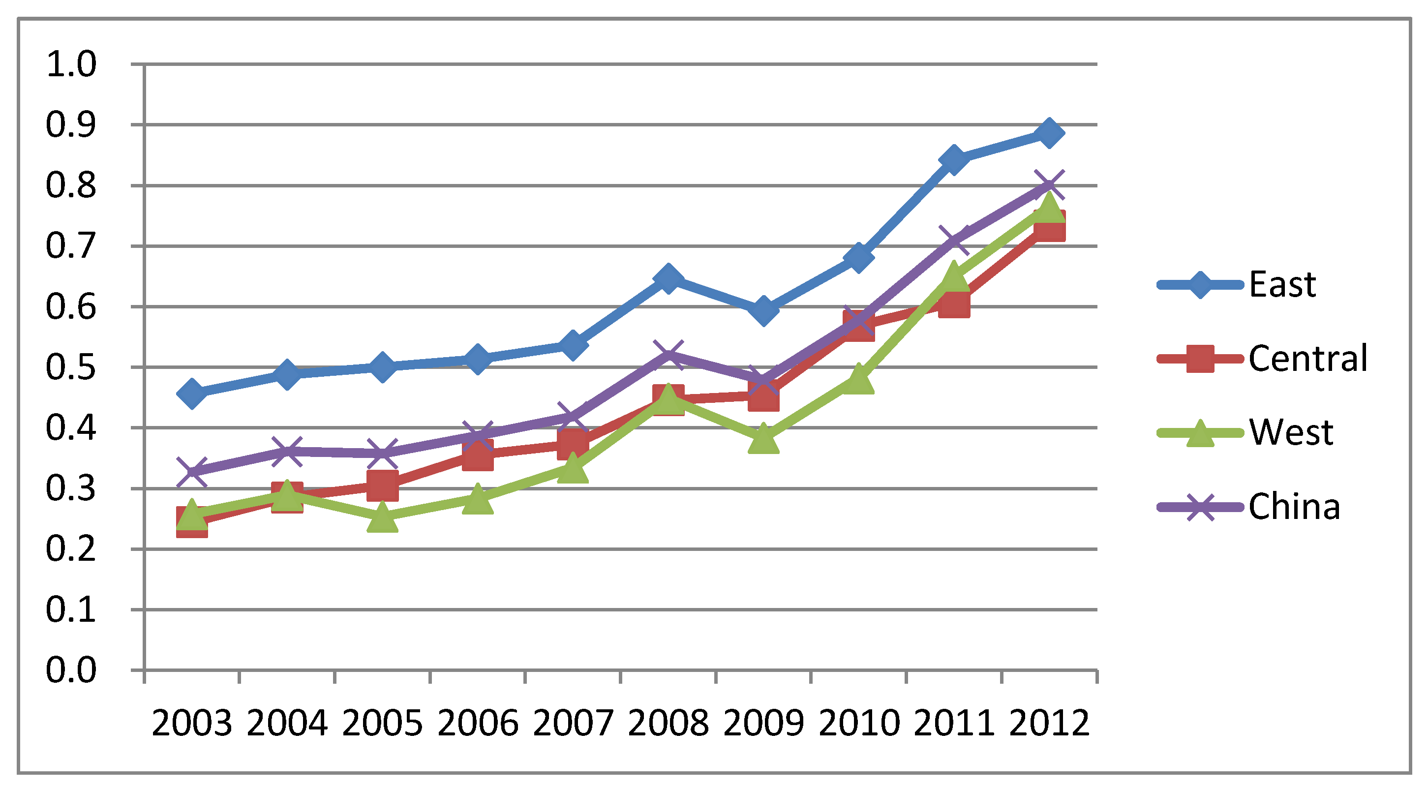
Firstly, the TCPILs for China and its three regions showed rising trends over the study period, and the eastern region performed much better in TCPIL than the central and western regions. However, all three regions have a large potential for improving their TCPILs. Most of the provinces in the eastern region (e.g., Hainan, Zhejiang and Guangdong) enjoyed better TCPILs, whereas those from the central and western regions (e.g., Gansu and Ningxia) suffered worse TCPILs.
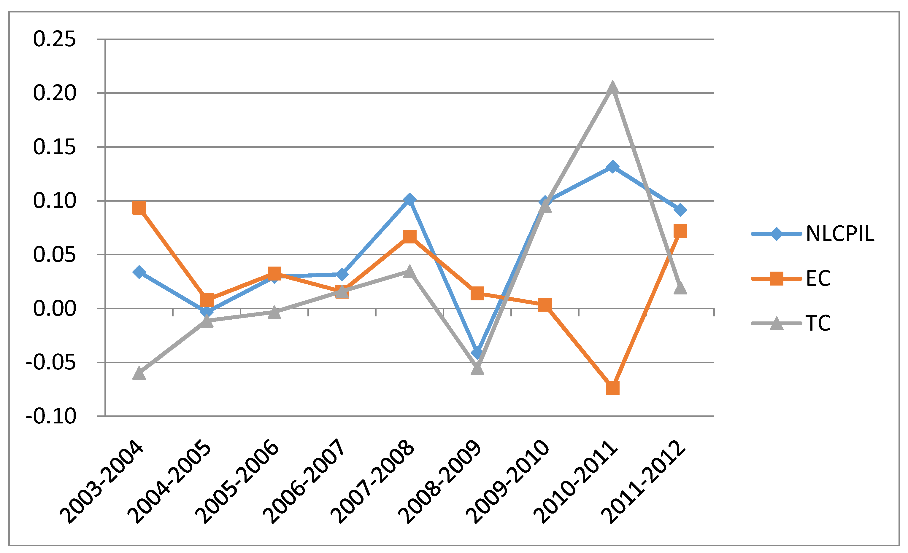
Secondly, the NLCPILs for China were greater than zero in most years of the study period, and their growth was mainly driven by ECs before 2009 and by TC subsequently. The eastern and central regions showed higher TCs, whereas the western region had a better EC performance. Many provinces with poor TCPILs had higher NLCPILs, which indicates that the regional gaps in TCPIL clearly showed a narrowing trend. In addition, most of the provinces that were identified as innovators of environmentally friendly industrial production technologies were in the eastern region (e.g., Beijing, Guangdong and Shandong).
Lastly, the results of the influencing factor analysis showed that the carbon emission reduction policies since 2009 have performed as expected, and they are helpful to improve the NLCPIL, which recommends the environmental protection policies. The EI, ES and LS indicators had expected significantly negative impacts on the NLCPIL, which means that the NLCPIL could be improved by saving more fossil energy, optimizing the energy structure by reducing the use of coal and properly solving the problem of surplus labor in the industrial sectors. The RI had an expected significantly positive impact on the NLCPIL, which implies that more investment in industrial R&D is needed. However, the FI and IS indices influenced the NLCPIL opposite the expected impacts, which had negative and positive signs, respectively. This may due to incomplete learning of foreign advanced production technologies and the fact that China has not yet fully entered into the stage of middle and late industrialization.
Based on the empirical analysis, we put forward some policy implications. Firstly, the central government of China should issue more policies on low-carbon and energy-saving industrial production to effectively protect the environment given rapid industrial economic development. In addition, the central government should strictly regulate local governments to fully implement those policies. Therefore, severe punishments for local government officials such as removing administrative duties or cutting their powers are necessary. Secondly, industrial enterprises should further optimize energy structures by reducing the use of coal and increasing the use of clean energy such as nuclear and wind power. The government should spend more money on the R&D of clean energy, subsidize enterprises that use clean energy, and promote cooperation between enterprises and research institutes. Third, we should carefully study advanced industrial production and management technologies by introducing foreign investment and industrial enterprises and by trying to develop our own technologies, especially for the regions with underdeveloped environmentally friendly industrial production technology. Lastly, the regional gaps in industrial production technology and environmental protection deserve more attention, and the central government of China should create more opportunities for underdeveloped provinces to communicate with developed provinces and introduce necessary technologies and talent. This study also has some limitations. Firstly, we only adopted a ten-year sample period because of the unavailability of data. We will try to obtain more data to extend the study period to produce more convincing and meaningful results. Secondly, some factors that play important roles in determining the efficiency of industrial land use were not considered in this paper for the same reason, such as the price of industrial land, carbon emissions trading costs and human capital. We will make these improvements in future studies.

Acknowledgments

This study was supported by the National Natural Science Foundation of China, No. 41561040; the Key projects of the National Social Science Fund of China, No. 15AZD075; the Key projects of the social science fund of Jiangxi Province in China “Study on the green utilization of land resources in China”; the Natural Science Foundation of Jiangxi Province No. 20143ACB21023; the Technology Foundation of Jiangxi Education Department of China, No. KJLD14033; the Fok Ying-Tung Fund, No. 141084; the graduate innovation fund project of Jiangxi university of finance and economics of China, No.XS295, No.XS308; the graduate innovation special funds project of Jiangxi province of China, No.YC2015-S217.

Author Contributions

Wei Wang and Hualin Xie had the original idea for the study. Wei Wang was responsible for data collecting. Wei Wang, Tong Jiang, Xue Xie, Daobei Zhang and Hualin Xie carried out the analyses. All the authors drafted the manuscript, and approved the final one.

Conflicts of Interest

The authors declare no conflict of interest.

References

  1. Jiang, F. The dynamic mechanism transform of China’s industrial economic growth. China Ind. Econ. 2014, 5, 5–17. (In Chinese) [Google Scholar]
  2. Che, L.; Han, X.; Zhao, L.; Wu, X. Coal use efficiency evaluation and decoupling analysis between coal use efficiency and economic growth in China. China Popul. Resour. Environ. 2015, 3, 104–110. (In Chinese) [Google Scholar]
  3. Tollefson, J. Gas to displace coal on road to clean energy. Nature 2010, 466, 19. [Google Scholar] [CrossRef] [PubMed]
  4. Choi, Y.; Zhang, N.; Zhou, P. Efficiency and abatement costs of energy-related CO2 emissions in China: A slacks-based efficiency measure. Appl. Energy 2012, 98, 198–208. [Google Scholar] [CrossRef]
  5. Liu, L.; Zong, H.; Zhao, E.; Chen, C.; Wang, J. Can China realize its carbon emission reduction goal in 2020: From the perspective of thermal power development. Appl. Energy 2014, 124, 199–212. [Google Scholar] [CrossRef]
  6. Ministry of Environmental Protection of the People’s Republic of China (MEPPRC). Available online: http://www.zhb.gov.cn/gkml/hbb/gwy/200910/t20091030_180716.htm (accessed on 30 October 2009). (In Chinese)
  7. Li, Y. Analysis of the mechanism and process of social conflicts in China’s urbanization. China Popul. Resour. Environ. 2015, 2, 57–65. (In Chinese) [Google Scholar]
  8. Cui, L.B.; Fan, Y.; Zhu, L.; Bi, Q.H. How Will the Emissions Trading Scheme Save Cost for Achieving China’s 2020 Carbon Intensity Reduction Target? Appl. Energy 2014, 136, 1043–1052. [Google Scholar] [CrossRef]
  9. Xie, H.; Wang, W. Spatiotemporal differences and convergence of urban industrial land use efficiency for China’s major economic zones. J. Geogr. Sci. 2015, 25, 1183–1198. [Google Scholar] [CrossRef]
  10. Lu, C.; Wen, F.; Yang, Q.; Zhang, P. Characteristics and driving factors of urban land use structure of cities at provincial level and above. Scientia Geographica Sinica 2011, 5, 599–607. [Google Scholar]
  11. Zhao, X.; Huang, X.; Ma, W.; Zhang, X. Identification method and treatment suggestion for idle land. China Land Sci. 2011, 9, 3–7. (In Chinese) [Google Scholar]
  12. Li, Y.; Shu, B.; Wu, Q. Urban Land Use Efficiency in China: Spatial and Temporal Characteristics, Regional Difference and Influence Factors. Econ. Geogr. 2014, 34, 133–139. (In Chinese) [Google Scholar]
  13. Huang, D.; Hong, L.; Liang, J. Analysis and evaluation of industrial land efficiency and intensive use in Fujian Province. Acta Geogr. Sin. 2009, 64, 479–486. (In Chinese) [Google Scholar]
  14. Hu, J.; Wang, S.; Yeh, F. Total-factor water efficiency of regions in China. Resour. Policy 2006, 31, 217–230. [Google Scholar] [CrossRef]
  15. Chen, W.; Peng, J.; Wu, Q. Spatial and temporal differences in industrial land use efficiency in China. Resour. Sci. 2014, 36, 2046–2056. (In Chinese) [Google Scholar]
  16. Xiong, Q.; Guo, G. Study on the efficiency difference of city industrial land production across provinces in China. Resour. Sci. 2013, 35, 910–917. (In Chinese) [Google Scholar]
  17. Guo, G.; Wen, Q. Industrial land productivity research under the environmental restriction based on unexpected outputs of 33 typical cities in China. China Popul. Resour. Environ. 2014, 24, 121–127. (In Chinese) [Google Scholar]
  18. Xie, H.; Wang, W. Exploring the spatial-temporal disparities of urban land use economic efficiency in China and its influencing factors under environmental constraints based on a sequential slacks-based model. Sustainability 2015, 7, 10171–10190. [Google Scholar] [CrossRef]
  19. Zhang, N.; Kong, F.; Choi, Y. Measuring sustainability performance for China: A sequential generalized directional distance function approach. Econ. Model. 2014, 41, 392–397. [Google Scholar] [CrossRef]
  20. Zhang, N.; Kong, F.; Choi, Y.; Zhou, P. The effect of size-control policy on unified energy and carbon efficiency for Chinese fossil fuel power plants. Energy Policy 2014, 70, 193–200. [Google Scholar] [CrossRef]
  21. Chung, Y.H.; Färe, R.; Grosskopf, S. Productivity and undesirable outputs: A directional distance function approach. J. Environ. Manag. 1997, 51, 229–240. [Google Scholar] [CrossRef]
  22. Kumar, S. Environmentally sensitive productivity growth: A global analysis using Malmquist-Luenberger index. Ecol. Econo. 2006, 56, 280–293. [Google Scholar] [CrossRef]
  23. Fan, M.; Shao, S.; Yang, L. Combining global Malmquist-Luenberger index and generalized method of moments to investigate industrial total factor CO2 emission performance: A case of Shanghai (China). Energy Policy 2015, 79, 189–201. [Google Scholar] [CrossRef]
  24. Arabi, B.; Munisamy, S.; Emrouznejad, A.; Shadman, F. Power industry restructuring and eco-efficiency changes: A new slacks-based model in Malmquist-Luenberger Index measurement. Energy Policy 2014, 68, 132–145. [Google Scholar] [CrossRef]
  25. Boussemart, J.P.; Briec, W.; Kerstens, K.; Poutineau, J.C. Luenberger and Malmquist productivity indices: Theoretical comparisons and empirical illustration. Bull. Econ. Res. 2003, 55, 391–405. [Google Scholar] [CrossRef]
  26. Chang, T.P.; Hu, J.L. Total-factor energy productivity growth, technical progress, and efficiency change: An empirical study of China. Appl. Energy 2010, 87, 3262–3270. [Google Scholar] [CrossRef]
  27. Chang, Y.; Zhang, N.; Danao, D.; Zhang, N. Environmental efficiency analysis of transportation system in China: A non-radial DEA approach. Energy Policy 2013, 58, 277–283. [Google Scholar] [CrossRef]
  28. Zhang, N.; Wei, X. Dynamic total-factor carbon emissions performance changes in the Chinese transportation industry. Appl. Energy 2015, 146, 409–420. [Google Scholar] [CrossRef]
  29. You, H.; Wu, C. Carbon emission efficiency and low carbon optimization of land use: Based on the perspective of energy consumption. J. Nat. Sources 2010, 25, 1875–1886. (In Chinese) [Google Scholar]
  30. Cui, Y.; Miao, J.; Yang, J. Empirical study on the eco-efficiency of urban non-agricultural land considering carbon emission. Syst. Eng. 2012, 30, 10–18. (In Chinese) [Google Scholar]
  31. Färe, R.; Grosskopf, S. New Directions: Efficiency and Productivity; Springer: New York, NY, USA, 2005. [Google Scholar]
  32. Mei, G.; Gan, J.; Zhang, N. Metafrontier environmental efficiency for China’s regions: a slack-based efficiency measure. Sustainability 2015, 7, 4004–4021. [Google Scholar] [CrossRef]
  33. Chambers, R.G.; Chung, Y.; Färe, R. Benefit and distance functions. J. Econ. Theory 1996, 70, 407–419. [Google Scholar] [CrossRef]
  34. Zhou, P.; Ang, B.W.; Wang, H. Energy and CO2 emission performance in electricity generation: A non-radial directional distance function approach. Eur. J. Oper. Res. 2012, 221, 625–635. [Google Scholar] [CrossRef]
  35. Oh, D. A metafrontier approach for measuring an environmentally sensitive productivity growth index. Energy Econ. 2010, 32, 146–157. [Google Scholar] [CrossRef]
  36. National Bureau of Statistics of China (NBSC). Available online: http://www.stats.gov.cn/tjsj/ndsj/ (accessed on 12 March 2015). (In Chinese)
  37. Zhang, N.; Kong, F.; Yu, Y. Measuring ecological total-factor energy efficiency incorporating regional heterogeneities in China. Ecol. Indic. 2015, 51, 165–172. [Google Scholar] [CrossRef]
  38. Wu, Y. China’s Capital Stock Series by Region and Sector; The University of Western Australia Discussion Paper; University of Western Australia: Perth, Australia, 2009. [Google Scholar]
  39. Zhang, N.; Choi, Y. Environmental energy efficiency of China’s regional economies: A non-oriented slacks-based measure analysis. Soc. Sci. J. 2013, 50, 225–234. [Google Scholar] [CrossRef]
  40. Du, L.; Wei, C.; Cai, S. Economic development and carbon dioxide emissions in China: Provincial panel data analysis. China Econ. Rev. 2012, 23, 371–384. [Google Scholar] [CrossRef]
  41. National Bureau of Statistics of China (NBSC). Available online: http://tongji.cnki.net/kns55/Navi/HomePage.aspx?id=N2010042092&name=YZGCA&floor=1 (accessed on 1 April 2015). (In Chinese)
  42. National Bureau of Statistics of China (NBSC). Available online: http://tongji.cnki.net/kns55/Navi/HomePage.aspx?id=N2010080088&name=YCXME&floor=1 (accessed on 1 November 2015). (In Chinese)
  43. Liu, N.; Ma, Z.; Kang, J. Changes in carbon intensity in China’s industrial sector: Decomposition and attribution analysis. Energy Policy 2015, 87, 28–38. [Google Scholar] [CrossRef]
  44. Chu, N.Y.; Li, S.K.; Ki, T.S. The Incidence of Surplus Labor in Rural China: A Nonparametric Estimation. J. Comp. Econ. 2000, 28, 565–580. [Google Scholar]
  45. Qin, H.; Su, Q.; Khu, S.; Tang, N. Water Quality changes during rapid urbanization in the Shenzhen river catchment: an integrated view of socio-economic and infrastructure development. Sustainability 2014, 6, 7433–7451. [Google Scholar] [CrossRef]
  46. Ouyang, M.; Peng, Y. The treatment-effect estimation: A case study of the 2008 economic stimulus package of China. J. Econ. 2015, 188, 545–557. [Google Scholar] [CrossRef]
  47. Zheng, S.; Yi, H.; Li, H. The impacts of provincial energy and environmental policies on air pollution control in China. Renew. Sustain. Energy Rev. 2015, 49, 386–394. [Google Scholar] [CrossRef]
  48. Porter, M.; van der Linde, C. Toward a new conception of the environment: Competitiveness relationship. J. Econ. Perspect. 1995, 9, 120–134. [Google Scholar] [CrossRef]
  49. Färe, R.; Grosskopf, S.; Norris, M.; Zhang, Z. Productivity growth, technical progress, and efficiency change in industrialized countries. Am. Econ. Rev. 1994, 84, 66–83. [Google Scholar]
  50. Balsalobre, D.; Álvarez, A.; Cantos, J.M. Public budgets for energy RD&D and the effects on energy intensity and pollution levels. Environ. Sci. Pollut. Res. 2014, 22, 4881–4892. [Google Scholar]
  51. Tang, L.; Li, R.; Tokimatsu, K.; Itsubo, N. Development of human health damage factors related to CO2 emissions by considering future socioeconomic scenarios. Int. J. Life Cycle Assess. 2015, 9, 1–12. [Google Scholar]
  52. Lu, F.; Feng, K. Why is autonomous product development the best way to learn foreign technology?—Lessons from the historical experiences of Japan’s and South Korea’s auto industries. Chin. Soft Sci. 2004, 4, 6–11. (In Chinese) [Google Scholar]
  53. Zhang, Y.; Xu, Q.; Wu, J. A Successful Anti-poverty War: Experience from China. Econ. Res. J. 2012, 11, 76–87. (In Chinese) [Google Scholar]
Figure 1. Trends in total-factor carbon emission performance of industrial land use (TCPIL) for China and its three regions, 2003–2012.
Sustainability 08 00336 g001
Figure 2. Trends in non-radial Luenberger carbon emission performance of industrial land use (NLCPIL) and its decomposition indices for China, 2003–2013, including efficiency change (EC) and technological change (TC).
Sustainability 08 00336 g002
Table 1. Descriptions of the influential factors.
VariableDefinitionDescriptionExpected Effect
EIEnergy intensityThe share of fossil energy used for industrial production in the total consumption in the countryNegative
ESEnergy structureThe share of coal consumption in the total fossil energy consumption for industrial productionNegative
RIResearch and development intensityThe share of investment in industrial research and development in the industrial GDPPositive
FIForeign funded industrial enterprises introductionThe share of GDP produced by foreign funded industrial enterprises in the national industrial GDPPositive
LSIndustrial labor shareThe share of workers in industrial sectors in the total number of workers nationwideNegative
ISIndustrial GDP shareThe share of GDP in industrial sectors in the total GDPNegative
POLCarbon emission reduction policyThe ambitious policies to reduce carbon emissions since 2009Positive
Table 2. TCPIL at the provincial level for all three regions, East (E), Central (C) and West (W) China 2003–2012.
ProvinceRegion2003200420052006200720082009201020112012Mean
BeijingE0.23750.29770.35400.32880.33510.35230.37150.38610.84881.00000.4512
TianjinE0.33040.36920.46790.51510.55880.63910.62520.74520.91011.00000.6161
HebeiE0.30730.35810.33660.38780.43010.47630.46310.54530.79001.00000.5095
LiaoningE0.18750.22130.26340.28450.35190.51350.41350.46370.49150.51430.3705
ShanghaiE0.34830.37070.36540.38700.40480.44370.39910.41140.40310.38640.3920
JiangsuE0.52310.50410.48880.52450.55360.59390.64490.71381.00001.00000.6547
ZhejiangE0.61410.58000.58790.63690.68540.75530.74690.87621.00001.00000.7483
FujianE0.59820.66070.56790.64940.63200.73540.72450.79741.00000.97300.7339
ShandongE0.41530.44880.44580.48730.54010.59890.63090.70080.82070.87750.5966
GuangdongE0.45880.55640.62410.68140.68801.00000.50390.84631.00001.00000.7359
HainanE1.00001.00001.00000.76510.72031.00001.00001.00001.00001.00000.9485
ShanxiC0.17710.23250.32120.32300.38290.46180.41190.52120.63520.58560.4052
JilinC0.17620.21360.22250.24310.30490.37190.40370.46220.53130.64730.3577
HeilongjiangC0.30260.35600.31110.32750.31930.37010.33360.43560.53790.54650.3840
AnhuiC0.21020.25740.24770.32830.32230.37870.41400.50770.45790.75010.3874
JiangxiC0.25880.30630.40820.54910.45590.50520.53560.67490.68100.79080.5166
HenanC0.31560.35680.40970.41460.49170.61140.60660.83830.99341.00000.6038
HubeiC0.25360.27330.23780.31900.32210.36280.42280.43510.42650.54710.3600
HunanC0.26280.28550.27940.33820.38390.50390.50090.67230.59731.00000.4824
Inner MongoliaW0.16850.22260.27420.31090.38360.47660.48950.70981.00001.00000.5036
GuangxiW0.21030.25570.27720.31310.38240.65160.48840.67880.82720.87750.4962
ChongqingW0.18100.21930.18390.21950.25580.30810.33110.37270.43080.53730.3040
SichuanW0.15080.18010.20010.26600.31640.33510.35160.37450.49270.66460.3332
GuizhouW0.16470.17460.21140.23840.28400.35400.34270.39870.36630.54190.3077
YunnanW0.32510.42840.35470.38300.35620.39840.38200.46720.51720.95540.4568
ShaanxiW0.24760.22140.34290.40500.40491.00000.53250.61410.69561.00000.5464
GansuW0.15020.18410.17820.20640.24430.28100.27460.36200.39970.42530.2706
QinghaiW1.00001.00000.42770.41280.52400.52420.51250.60081.00001.00000.7002
NingxiaW0.09590.14450.13570.15760.30690.23050.27300.39900.43220.41200.2587
XinjiangW0.14100.15070.20410.20690.22110.37130.24270.32381.00001.00000.3862
East 0.45640.48790.50020.51340.53640.64620.59300.68060.84220.88650.6143
Central 0.24460.28520.30470.35540.37290.44570.45360.56840.60760.73340.4371
West 0.25770.28920.25360.28360.33450.44830.38370.48190.65110.76490.4149
China 0.32710.36100.35770.38700.41880.52020.47910.57780.70950.80110.4939
Table 3. NLCPIL and its decomposition indices for the three regions.
NLCPILECTC
E0.04780.01220.0356
C0.05430.01870.0357
W0.05630.04460.0117
China0.05270.02580.0268
Table 4. Changes in the NLCPIL at the provincial level, 2003–2012. Positive values are marked grey.
ProvinceRegion03–0404–0505–0606–0707–0808–0909–1010–1111–12Mean
BeijingE0.06010.0563−0.02520.00630.01720.01910.01470.46270.15120.0847
TianjinE0.03880.09870.04720.04370.0803−0.01390.12010.16480.08990.0744
HebeiE0.0508−0.02150.05120.04230.0462−0.01320.08220.24470.21000.0770
LiaoningE0.03380.04210.02110.06740.1616−0.10000.05030.02770.02290.0363
ShanghaiE0.0224−0.00530.02160.01770.0390−0.04470.0123−0.0083−0.01670.0042
JiangsuE−0.0190−0.01520.03570.02900.04030.05100.06890.28620.00000.0530
ZhejiangE−0.03410.00790.04900.04850.0700−0.00840.12920.12380.00000.0429
FujianE0.0624−0.09270.0814−0.01740.1034−0.01090.07290.2026−0.02700.0416
ShandongE0.0335−0.00290.04150.05280.05880.03200.06990.11990.05680.0514
GuangdongE0.09760.06770.05730.00660.3120−0.49610.34240.15370.00000.0601
HainanE0.00000.0000−0.2349−0.04480.27970.00000.00000.00000.00000.0000
ShanxiC0.05530.08870.00180.05990.0789−0.04990.10940.1140−0.04960.0454
JilinC0.03740.00890.02060.06180.06700.03180.05850.06910.11610.0524
HeilongjiangC0.0534−0.04500.0165−0.00820.0508−0.03650.10200.10230.00870.0271
AnhuiC0.0472−0.00970.0806−0.00610.05650.03530.0937−0.04980.29220.0600
JiangxiC0.04750.10190.1408−0.09310.04920.03040.13930.00610.10990.0591
HenanC0.04120.05290.00490.07700.1197−0.00480.23170.15510.00660.0760
HubeiC0.0197−0.03550.08120.00320.04070.06000.0123−0.00860.12060.0326
HunanC0.0227−0.00610.05890.04570.1199−0.00300.1714−0.07500.40270.0819
Inner MongoliaW0.05410.05160.03670.07270.09310.01290.22040.29020.00000.0924
GuangxiW0.04540.02150.03590.06930.2692−0.16320.19030.14840.05030.0741
ChongqingW0.0382−0.03530.03560.03630.05230.02300.04150.05810.10650.0396
SichuanW0.02930.02000.06600.05040.01870.01650.02290.11820.17190.0571
GuizhouW0.00990.03680.02700.04570.0700−0.01130.0560−0.03230.17560.0419
YunnanW0.1033−0.07370.0282−0.02680.0421−0.01630.08510.05010.43820.0700
ShaanxiW−0.02620.12150.06210.00000.5951−0.46750.08160.08150.30440.0836
GansuW0.0339−0.00590.02820.03790.0366−0.00640.08740.03770.02560.0306
QinghaiW0.0000−0.5723−0.01490.11120.0002−0.01170.08830.39920.00000.0000
NingxiaW0.0486−0.00880.02190.1492−0.07640.04250.12600.0333−0.02020.0351
XinjiangW0.00970.05340.00270.01420.1502−0.12860.08110.67620.00000.0954
China 0.0339−0.00330.02940.03170.1014−0.04110.09870.13170.09160.0527
Table 5. EC component of the NLCPIL at the provincial level, 2003–2012. Positive values are marked grey.
ProvinceRegion03–0404–0505–0606–0707–0808–0909–1010–1111–12Mean
BeijingE0.55510.00000.00000.00000.00000.00000.00000.00000.00000.0617
TianjinE0.05100.2648−0.06500.06500.00000.00000.00000.00000.00000.0351
HebeiE0.43580.00000.00000.00000.0000−0.17400.17400.00000.00000.0484
LiaoningE0.05400.0712−0.02470.08790.1145−0.05130.0157−0.0547−0.03040.0202
ShanghaiE0.3374−0.37150.37150.00000.00000.0000−0.2716−0.31850.0849−0.0186
JiangsuE0.00000.00000.00000.00000.00000.00000.00000.00000.00000.0000
ZhejiangE0.00000.00000.00000.00000.00000.00000.00000.00000.00000.0000
FujianE0.00000.00000.00000.00000.00000.00000.00000.00000.00000.0000
ShandongE0.00000.00000.00000.00000.00000.00000.00000.0000−0.1107−0.0123
GuangdongE0.00000.00000.00000.00000.00000.00000.00000.00000.00000.0000
HainanE0.00000.00000.00000.00000.00000.00000.00000.00000.00000.0000
ShanxiC0.04850.2033−0.04500.12340.0357−0.05960.0758−0.0042−0.09500.0314
JilinC0.09160.0117−0.00080.07940.07260.06130.0103−0.09890.14260.0411
HeilongjiangC0.00000.00000.0000−0.45540.24940.09030.1157−0.41300.1757−0.0264
AnhuiC0.10390.00450.0937−0.04370.08790.07180.0004−0.18600.26570.0442
JiangxiC0.00000.00000.00000.00000.00000.00000.00000.0000−0.0775−0.0086
HenanC0.00000.00000.00000.00000.00000.00000.00000.00000.00000.0000
HubeiC0.0183−0.03160.0774−0.00650.00700.0817−0.0252−0.09740.09200.0129
HunanC0.0578−0.01190.22000.04030.00910.05680.05060.06860.00000.0546
Inner MongoliaW0.10120.08270.02960.41760.00000.00000.00000.00000.00000.0701
GuangxiW0.4709−0.37780.02240.06500.29040.00000.00000.00000.00000.0523
ChongqingW−0.0714−0.04590.02960.03820.03980.1453−0.0147−0.10520.14470.0178
SichuanW0.03460.04530.06000.09220.02010.0352−0.07280.5161−0.29930.0479
GuizhouW0.03950.04810.0905−0.01960.23700.2228−0.1448−0.46280.60760.0687
YunnanW0.00000.00000.0000−0.34760.1191−0.05360.0953−0.24260.42940.0000
ShaanxiW−0.06780.25460.05610.00400.30340.00000.0000−0.18220.18220.0611
GansuW0.03660.04710.01460.05170.0815−0.00340.0951−0.17390.18360.0370
QinghaiW0.00000.00000.00000.00000.00000.00000.00000.00000.00000.0000
NingxiaW−0.13530.04730.04750.28120.33590.00000.0000−0.46360.46360.0641
XinjiangW0.64770.00000.00000.00000.00000.00000.00000.00000.00000.0720
China 0.09360.00810.03260.01580.06680.01410.0035−0.07390.07200.0258
Table 6. TC component of the NLCPIL at the provincial level, 2003–2012. Positive values are marked grey.
ProvinceRegionTCTCTCTCTCTCTCTCTCMean
BeijingE−0.49490.0563−0.02520.00630.01720.01920.01460.46270.15120.0230
TianjinE−0.0122−0.16610.1122−0.02130.0803−0.01390.12000.16490.08990.0393
HebeiE−0.3850−0.02150.05120.04230.04620.1608−0.09180.24470.21000.0285
LiaoningE−0.0202−0.02910.0458−0.02050.0471−0.04870.03450.08250.05320.0161
ShanghaiE−0.31500.3662−0.34990.01780.0389−0.04460.28390.3102−0.10160.0229
JiangsuE−0.0190−0.01530.03570.02910.04030.05100.06890.28620.00000.0530
ZhejiangE−0.03410.00790.04900.04850.0699−0.00840.12930.12380.00000.0429
FujianE0.0625−0.09280.0815−0.01740.1034−0.01090.07290.2026−0.02700.0416
ShandongE0.0335−0.00300.04150.05280.05880.03200.06990.11990.16750.0637
GuangdongE0.09760.06770.05730.00660.3120−0.49610.34240.15370.00000.0601
HainanE0.00000.0000−0.2349−0.04480.27970.00000.00000.00000.00000.0000
ShanxiC0.0069−0.11460.0468−0.06350.04320.00970.03350.11820.04540.0140
JilinC−0.0542−0.00280.0214−0.0176−0.0056−0.02950.04820.1680−0.02660.0113
HeilongjiangC0.0534−0.04490.01640.4472−0.1986−0.1268−0.01370.5153−0.16710.0535
AnhuiC−0.0567−0.0142−0.01310.0377−0.0315−0.03650.09330.13620.02650.0157
JiangxiC0.04750.10190.1409−0.09320.04930.03040.13930.00610.18730.0677
HenanC0.04120.05290.00490.07710.1197−0.00480.23170.15510.00660.0760
HubeiC0.0014−0.00390.00380.00960.0337−0.02170.03750.08880.02860.0198
HunanC−0.03510.0058−0.16120.00540.1109−0.05980.1208−0.14360.40270.0273
Inner MongoliaW−0.0471−0.03110.0071−0.34490.09300.01290.22030.29020.00000.0223
GuangxiW−0.42550.39930.01350.0043−0.0212−0.16320.19040.14840.05030.0218
ChongqingW0.10970.01050.0060−0.00190.0125−0.12230.05630.1633−0.03820.0218
SichuanW−0.0053−0.02530.0059−0.0418−0.0014−0.01870.0957−0.39790.47120.0092
GuizhouW−0.0296−0.0113−0.06350.0652−0.1670−0.23410.20080.4304−0.4320−0.0268
YunnanW0.1033−0.07370.02830.3208−0.07690.0372−0.01010.29260.00880.0700
ShaanxiW0.0416−0.13310.0060−0.00410.2917−0.46750.08160.26370.12220.0225
GansuW−0.0027−0.05300.0136−0.0138−0.0448−0.0030−0.00770.2116−0.1580−0.0064
QinghaiW0.0000−0.5723−0.01490.11120.0002−0.01170.08830.39920.00000.0000
NingxiaW0.1839−0.0561−0.0256−0.1319−0.41230.04250.12600.4968−0.4838−0.0289
XinjiangW−0.63800.05340.00280.01420.1502−0.12860.08110.67620.00000.0235
China −0.0597−0.0114−0.00320.01600.0346−0.05520.09530.20570.01960.0268
Table 7. Innovators in the eastern, central and western regions, 2003–2012.
PeriodEastCentralWest
2003–2004Shandong, Fujian, GuangdongHenan, Jiangxi, HeilongjiangYunnan
2004–2005Zhejiang, Beijing, GuangdongHenan, JiangxiXinjiang
2005–2006Jiangsu, Shandong, Zhejiang, Hebei, Guangdong, FujianHenan, Heilongjiang, JiangxiXinjiang, Yunnan
2006–2007Beijing, Guangdong, Shanghai, Jiangsu, Hebei, Zhejiang, ShandongHenanXinjiang, Qinghai
2007–2008Beijing, Shanghai, Jiangsu, Hebei, Shandong, Zhejiang, Tianjin, Fujian, Hainan, GuangdongJiangxi, HenanInner Mongolia, Xinjiang, Shaanxi
2008–2009Beijing, Shandong, JiangsuJiangxiInner Mongolia, Ningxia
2009–2010Beijing, Jiangsu, Shandong, Fujian, Tianjin, Zhejiang, GuangdongJiangxi, HenanXinjiang, Shaanxi, Qinghai, Ningxia, Guangxi, Inner Mongolia
2010–2011Shandong, Zhejiang, Guangdong, Tianjin, Fujian, Hebei, Jiangsu, BeijingJiangxi, HenanGuangxi, Inner Mongolia, Qinghai, Xinjiang
2011–2012Tianjin, Beijing, HebeiHenan, HunanGuangxi, Shaanxi, Yunnan
Table 8. Regression results. *** p < 0.001, ** p < 0.05, * p < 0.01.
Model 1Model 2Model 3Model 4
EI−0.0164 *** (−2.5946)−0.0173 *** (−2.6929)−0.0227 *** (−2.9775)−0.0144 ** (−1.9460)
ES−0.0013 *** (−3.4321)−0.0012 *** (−3.2012)−0.0019 *** (−4.7769)−0.0019 *** (−4.5950)
RI 0.0034 *** 3.7902)0.0134 *** (3.0684)0.0122 *** (2.6954)
FI −0.0001 ** (−2.2041)−0.0001 ** (−2.0582)−0.0001 ** (−2.0997)
LS −0.0024 *** (−7.3504)−0.0025 *** (−7.2698)
IS 0.0014 ** (2.3019)0.0015 ** (2.3484)
POL 0.0266 *** (3.1863)
Constant0.0696 *** (6.5035)0.0656 *** (4.3790)0.0935 *** (2.7554)0.0813 ** (2.3186)
Adjusted R20.06740.04870.28430.2329
F-statistic17.395015.44157.12335.6660
Prob.0.00000.00000.00000.0000

