3.1. Temporal/Spatial Similarity and Grouping
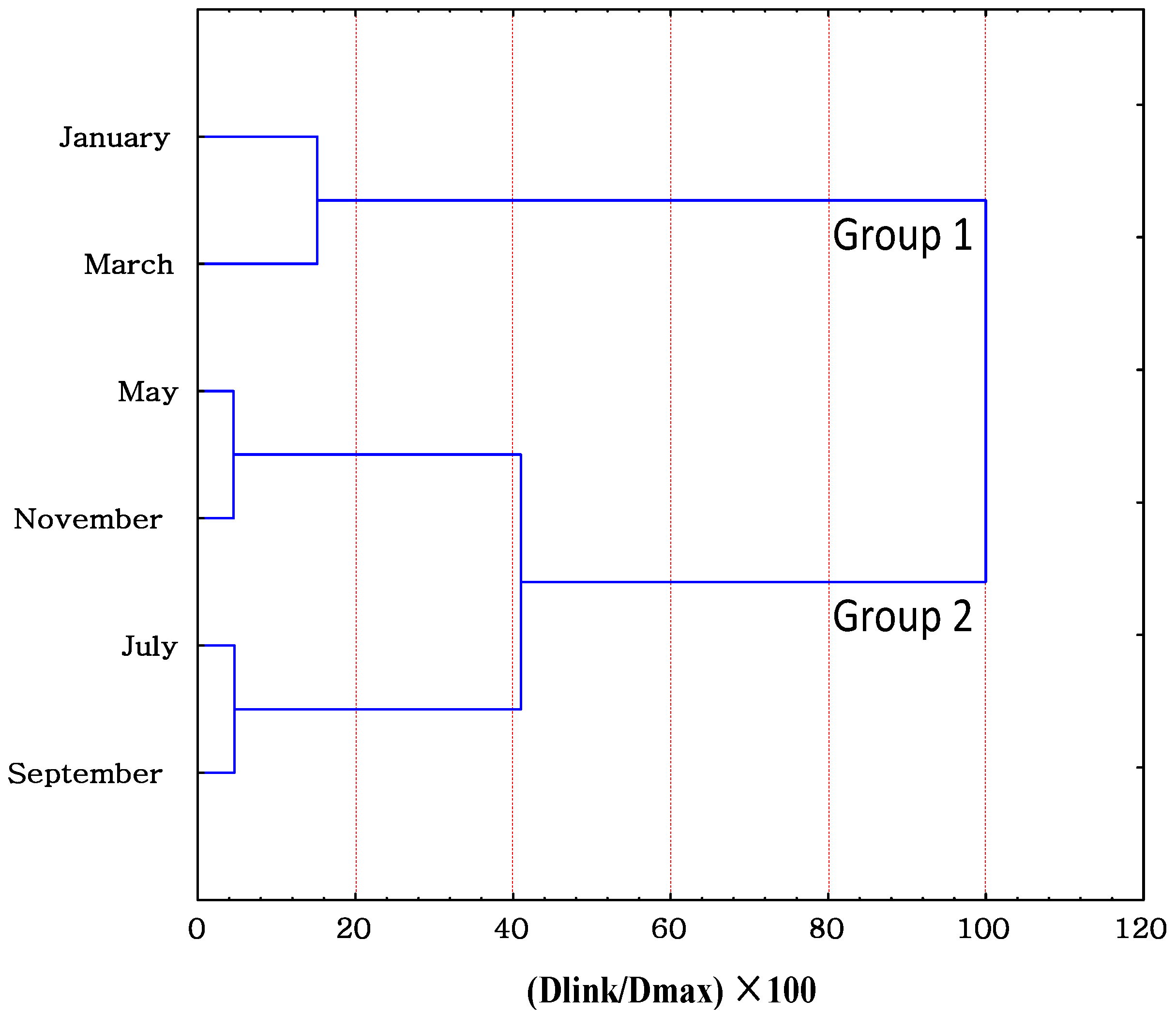
Figure 3 shows the results of temporal cluster analysis, grouping the 6 months into two statistically significant clusters at (D
link/D
max) × 100 < 60. Cluster 1 (dry season), comprised of January and March, approximately correspond to the low flow period. Cluster 2 (wet season) contains two small clusters at (D
link/D
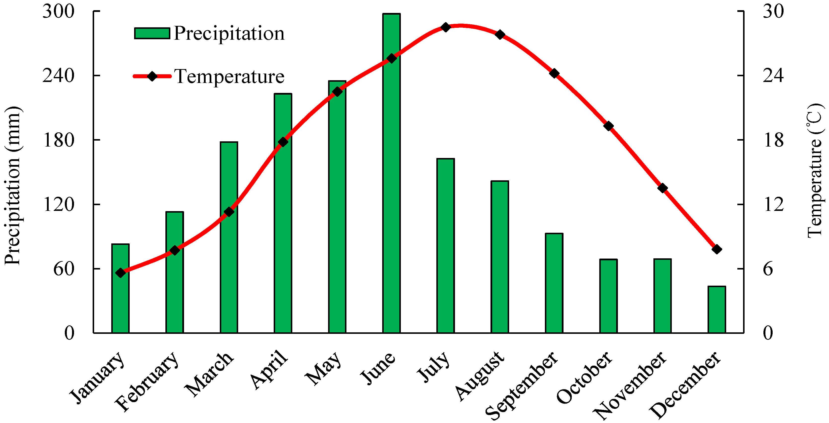
max) × 100 < 40; that is, May and November reflect the mean flow periods, and the remaining months (July and September) comprise another group, and reflect the high flow period. Notably, temporal variation of surface water quality was significantly affected by local climate seasons (spring, summer, autumn and winter) and hydrological conditions (low, mean, and high flow period). The Poyang Lake Basin lies in a subtropical wet climate zone with a distinct alternation from wet to a dry season, consistent with the temporal patterns of water quality (
Figure 3).
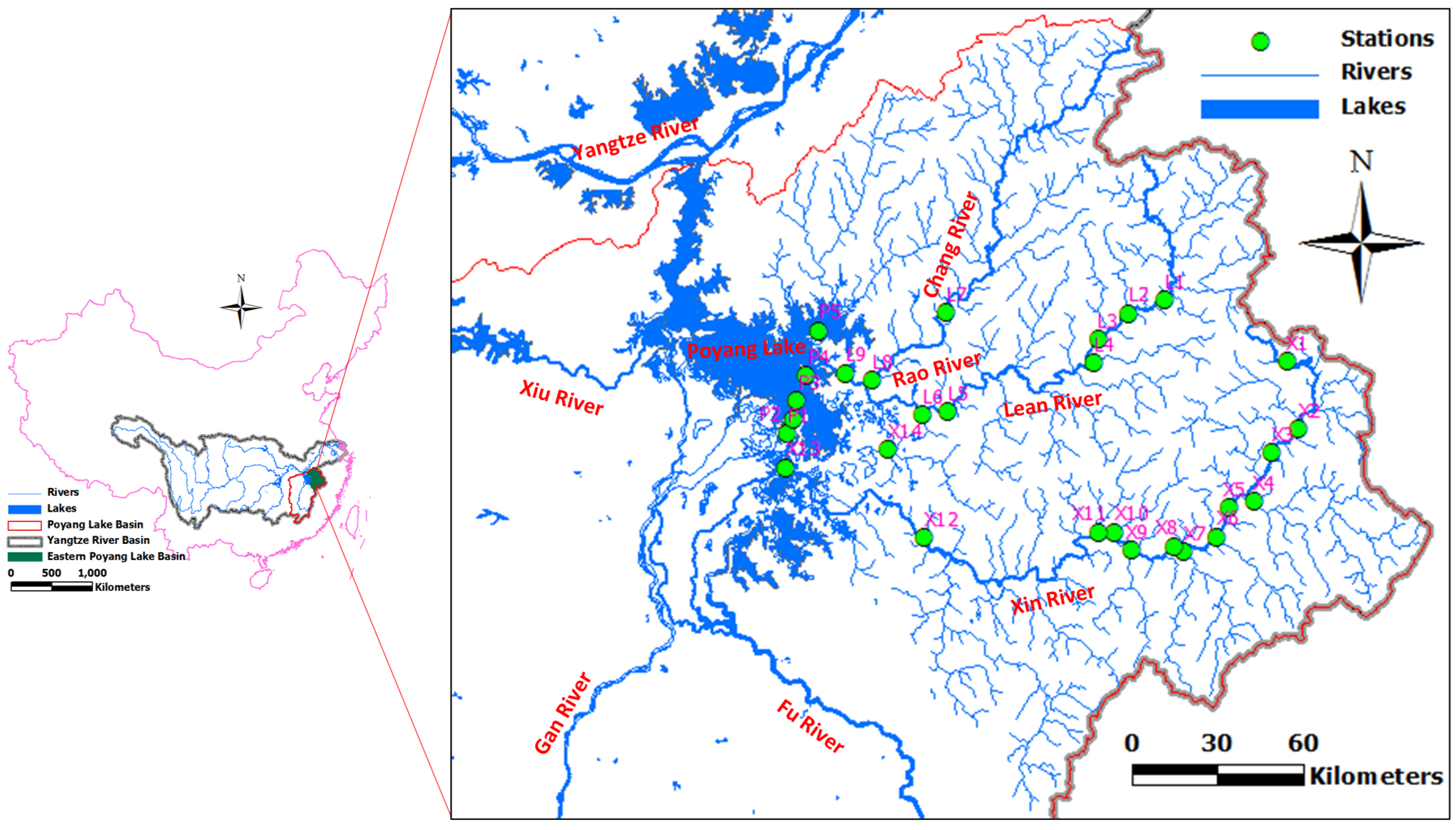
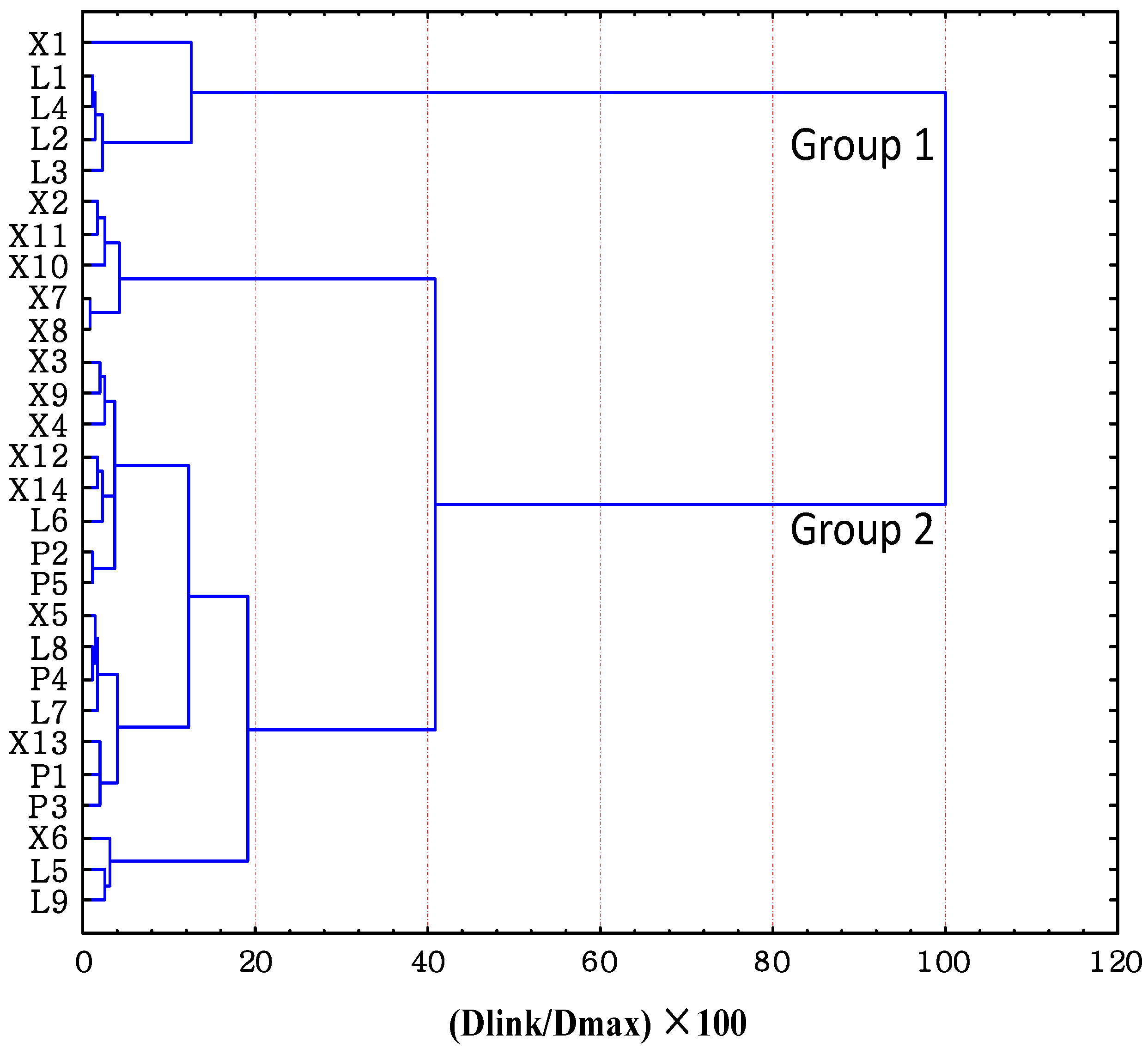
Spatial CA also yielded a dendrogram with two statistically significant clusters at (D
link/D
max) × 100 < 60 (
Figure 4). Group 1 included X1 and L1 to L4, and the
remaining monitoring stations comprised Group 2. The X1 station and L1 to L4 stations in Group 1 are located at the upstream of the Xin River and the Lean River, respectively, which, due to low population density and the absence of industrial and commercial activity, are far from major point and non-point pollution sources. However, L1–L4 stations are located in the Dexing district, which is one of the largest copper and gold producing districts in China and metal pollution and associated mineral pollution are always a problem [
39,
40]. Despite relatively high Cu, S, and F concentrations were observed at the L4 Station in this study, Group 1 should be considered as moderate or low pollution. Group 2 corresponds to highly polluted stations, with highest average concentrations of NH
4-N, oil, BOD, COD and TP. Most stations in this group were located at the middle to down-stream of the east Poyang Lake basin and received pollution from point sources including municipal sewage and industrial wastewater and non-point pollution sources.
Figure 3.
Dendogram showing the temporal clustering of study periods.
Figure 3.
Dendogram showing the temporal clustering of study periods.
Figure 4.
Dendogram showing spatial clustering of study periods.
Figure 4.
Dendogram showing spatial clustering of study periods.
3.2. Temporal/Spatial Variations in River Water Quality
Based on the temporal groups (wet season and dry season) from CA, DA was performed on raw data to further explore temporal changes in surface water quality.
Table 2 and
Table 3 indicate the discriminant functions (DFs) and classification matrices (CMs), which were calculated by the standard, forward stepwise and backward stepwise modes of DA. Variables are included step-by-step beginning with the more significant until no significant changes in the forward stepwise mode, but are removed step-by-step beginning with the less significant in the backward stepwise mode. Both the standard and forward stepwise mode DFs using 14 and 7 discriminant variables, respectively, produced the corresponding CMs assigning 96.43% of the cases correctly. In the backward stepwise mode, however, DA yielded a CM with approximately 97.86% correct assignations using only four discriminant parameters, showing that TEMP, pH, NH
4-N, and TN. Thus, the temporal DA indicated that TEMP, pH, NH
4-N, and TN were the most significant parameters to discriminate differences between the wet season and dry season, revealing that these four parameters could be used to account for the expected temporal changes in surface water quality in the Eastern Poyang Lake Basin.
Table 2.
Classification functions coefficients for DA of temporal changes.
Table 2.
Classification functions coefficients for DA of temporal changes.
| Parameters | Standard Mode | Forward Stepwise Mode | Backward Stepwise Mode |
|---|
| Wet Season | Dry Season | Wet Season | Dry Season | Wet Season | Dry Season |
|---|
| TEMP | 1.989 | 3.033 | 3.241 | 2.207 | 2.613 | 1.577 |
| pH | 82.847 | 84.585 | 59.995 | 58.095 | 56.048 | 54.185 |
| NH4-N | 21.105 | 24.167 | 28.602 | 25.452 | 27.846 | 25.129 |
| BOD | 9.934 | 10.125 | | | | |
| COD | −1.194 | −1.189 | | | | |
| DO | 10.981 | 10.727 | 12.409 | 12.687 | | |
| TN | −5.506 | −7.395 | −9.417 | −7.549 | −12.533 | −10.631 |
| TP | 7.996 | 6.712 | −3.095 | −1.832 | | |
| F | 46.734 | 46.243 | | | | |
| S | 631.996 | 634.440 | | | | |
| Cu | −255.025 | −250.116 | | | | |
| Oil | −148.788 | −206.928 | 20.532 | 75.009 | | |
| Cr | 374.404 | 403.601 | | | | |
| Zn | 53.327 | 52.592 | | | | |
| Constant | −378.134 | −403.979 | −302.864 | −276.639 | −235.610 | −206.896 |
Table 3.
Classification matrix for DA of temporal changes.
Table 3.
Classification matrix for DA of temporal changes.
| Monitoring Periods | Percent Correct | Temporal Groups |
|---|
| Wet Season | Dry Season |
|---|
| Standard mode |
| Wet Season | 95.536 | 321 | 15 |
| Dry Season | 100 | 0 | 224 |
| Total | 97.321 | 321 | 239 |
| Forward stepwise mode | | | |
| Wet Season | 95.536 | 321 | 15 |
| Dry Season | 100 | 0 | 224 |
| Total | 97.321 | 321 | 239 |
| Backward stepwise mode | | | |
| Wet Season | 96.429 | 324 | 12 |
| Dry Season | 100 | 0 | 224 |
| Total | 97.857 | 324 | 236 |
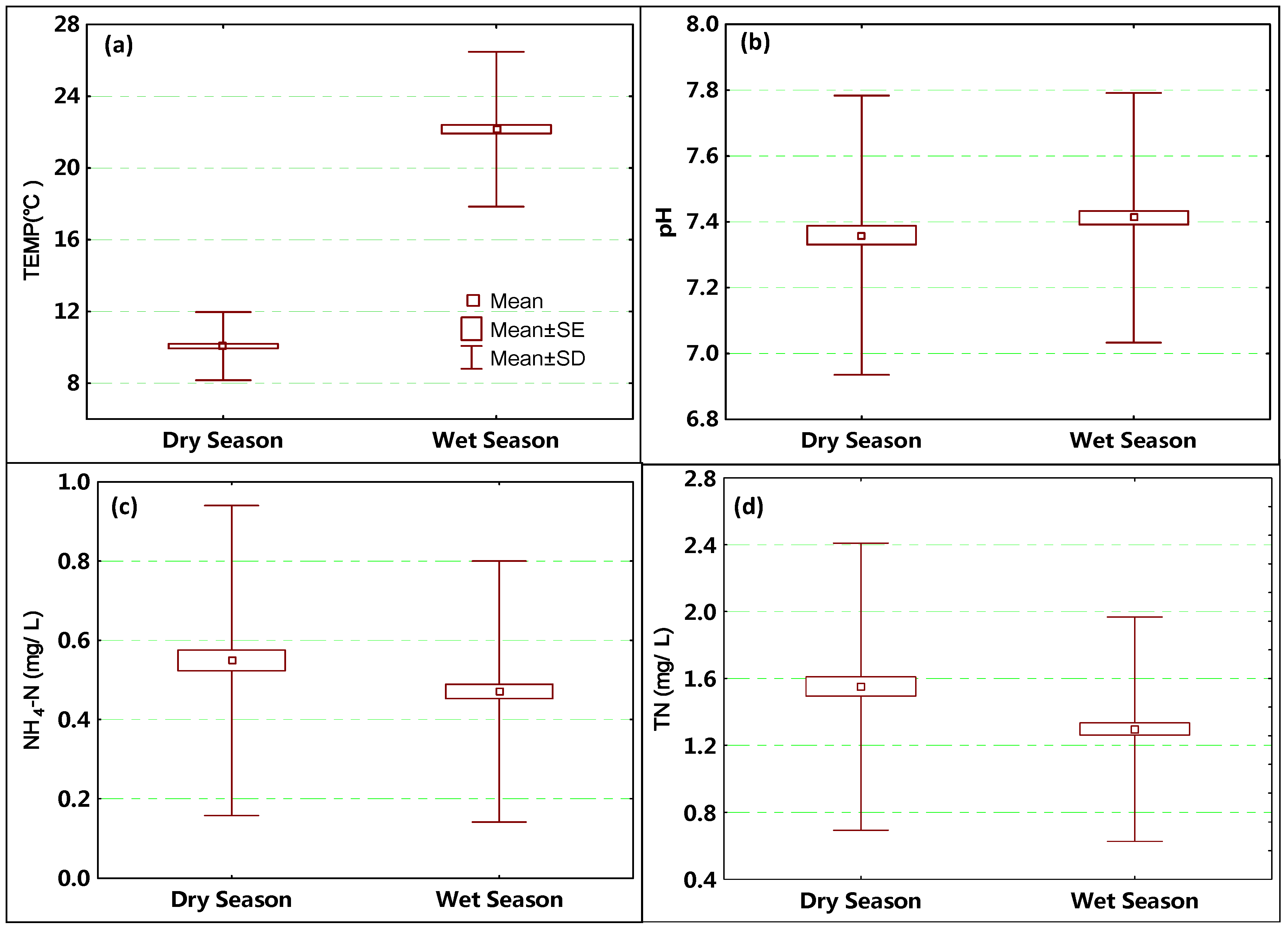
Box and whisker plots of the discriminate parameters identified by DA are indicated in
Figure 5. The average temperature (
Figure 5a) in wet season was clearly higher than in dry season because of the local climate. The same difference in pH was found in
Figure 5b. In contrast, the average NH
4-N and TN were higher in dry season than in wet season due to the local hydrologic conditions. The discharge in the wet season is much larger than in the dry season, which significantly dilutes the NH
4-N and TN. Moreover, in wet season (typical in summer and autumn) there are more aquatic organisms than in the dry season, consuming more NH
4-N.
Figure 5.
Temporal changes: (a) temperature; (b) pH; (c) NH4-N; and (d) TN in east Poyang Lake basin.
Figure 5.
Temporal changes: (a) temperature; (b) pH; (c) NH4-N; and (d) TN in east Poyang Lake basin.
Table 4.
Classification functions coefficients for DA of spatial changes.
Table 4.
Classification functions coefficients for DA of spatial changes.
| Parameters | Standard Mode | Forward Stepwise Mode | Backward Stepwise Mode |
|---|
| Low Pollution | High Pollution | Low Pollution | High Pollution | Low Pollution | High Pollution |
|---|
| TEMP | 1.028 | 1.07 | 1.214 | 1.260 | | |
| pH | 87.554 | 91.925 | 79.992 | 84.230 | 72.662 | 77.108 |
| NH4-N | 15.389 | 13.534 | 16.827 | 15.151 | | |
| BOD | 10.175 | 10.467 | | | | |
| COD | −0.833 | −0.584 | −0.409 | −0.146 | −0.376 | −0.146 |
| DO | 10.645 | 10.246 | 10.144 | 9.730 | | |
| TN | −1.196 | 0.484 | −0.140 | 1.573 | 3.971 | 5.296 |
| TP | 10.63 | 11.57 | | | | |
| F | 41.529 | 37.651 | 42.883 | 38.954 | 59.009 | 54.412 |
| S | 518.07 | 441.985 | 479.059 | 401.226 | 416.961 | 330.412 |
| Cu | −244.929 | −234.766 | −205.655 | −195.490 | | |
| Oil | −63.009 | −43.309 | 77.283 | 100.383 | | |
| Cr | 435.253 | 496.253 | 588.508 | 653.149 | | |
| Zn | 54.778 | 55.278 | | | | |
| Constant | −384.511 | −413.498 | −349.255 | −376.823 | −273.306 | −303.391 |
Just like temporal DA, the DFs and CMs for spatial DA were obtained from the standard, forward stepwise and backward stepwise modes on the basis of spatial groups (low pollution stations and high pollution stations), which are shown in
Table 4 and
Table 5. Both the standard and forward stepwise mode DFs using 14 and 11 discriminant variables, respectively, yielded the corresponding CMs assigning 95% of the cases correctly, whereas the backward stepwise DA gave CMs with about 93.75% correct assignations using only five discriminant parameters (
Table 4 and
Table 5). Backward stepwise DA showed that pH, COD, TN, F, and S were the most significant parameters to discriminate differences between the low pollution stations and high pollution stations.
Table 5.
Classification matrix for discriminant analysis of spatial changes.
Table 5.
Classification matrix for discriminant analysis of spatial changes.
| Monitoring Stations | Percent Correct | Spatial Groups |
|---|
| Low Pollution | High Pollution |
|---|
| Standard mode |
| Low pollution | 72.000 | 72 | 28 |
| High pollution | 100.000 | 0 | 460 |
| Total | 95.000 | 72 | 28 |
| Forward stepwise mode | | | |
| Low pollution | 72.000 | 72 | 28 |
| High pollution | 100.000 | 0 | 460 |
| Total | 95.000 | 72 | 488 |
| Backward stepwise mode | | | |
| Low pollution | 69.000 | 69 | 31 |
| High pollution | 99.130 | 4 | 456 |
| Total | 93.750 | 73 | 487 |
Table 6.
Loadings of experimental variables (14) on significant VFs for low pollution and high pollution.
Table 6.
Loadings of experimental variables (14) on significant VFs for low pollution and high pollution.
| Parameters | Low Pollution (Six Significant Principal Components) | High Pollution (four Significant Principal Components) |
|---|
| VF1 | VF2 | VF3 | VF4 | VF5 | VF6 | VF1 | VF2 | VF3 | VF4 |
|---|
| TEMP | 0.015 | 0.026 | 0.042 | 0.874 | 0.211 | 0.107 | 0.206 | −0.362 | −0.623 | −0.017 |
| pH | 0.730 | 0.230 | 0.201 | −0.068 | −0.243 | −0.169 | −0.657 | −0.149 | −0.114 | −0.081 |
| NH4-N | −0.144 | −0.078 | −0.032 | 0.084 | 0.934 | 0.058 | −0.069 | 0.861 | 0.022 | 0.038 |
| BOD | −0.013 | −0.834 | 0.036 | 0.167 | −0.040 | 0.249 | 0.103 | −0.054 | −0.365 | 0.701 |
| COD | 0.607 | −0.418 | 0.362 | −0.307 | 0.263 | −0.014 | 0.050 | 0.562 | 0.234 | 0.318 |
| DO | −0.172 | 0.197 | −0.214 | −0.745 | 0.138 | 0.165 | −0.165 | −0.107 | 0.794 | −0.012 |
| TN | 0.721 | 0.283 | −0.127 | 0.186 | 0.443 | −0.124 | 0.219 | 0.651 | −0.003 | 0.091 |
| TP | 0.149 | 0.355 | 0.758 | 0.097 | −0.040 | −0.091 | 0.466 | 0.413 | 0.157 | 0.179 |
| F | −0.597 | −0.440 | −0.121 | −0.253 | 0.387 | 0.261 | 0.330 | 0.113 | 0.646 | 0.065 |
| S | −0.779 | 0.139 | 0.067 | −0.152 | 0.155 | −0.052 | −0.664 | 0.364 | −0.095 | −0.178 |
| Cu | 0.094 | 0.741 | 0.156 | −0.023 | −0.109 | 0.334 | −0.831 | −0.079 | 0.224 | −0.055 |
| Oil | 0.420 | 0.021 | 0.611 | 0.165 | −0.253 | −0.126 | 0.131 | 0.202 | 0.026 | 0.626 |
| Cr | −0.188 | −0.154 | 0.887 | 0.075 | 0.065 | 0.117 | 0.073 | 0.129 | 0.266 | 0.639 |
| Zn | −0.123 | −0.011 | −0.026 | −0.017 | 0.061 | 0.931 | 0.835 | 0.098 | −0.169 | 0.073 |
| Eigenvalue | 3.553 | 2.000 | 1.709 | 1.469 | 1.302 | 1.007 | 3.205 | 2.364 | 1.426 | 1.094 |
| %Total variance | 25.382 | 14.287 | 12.208 | 10.491 | 9.303 | 7.190 | 22.890 | 16.883 | 10.189 | 7.817 |
| Cumulative% variance | 25.382 | 39.668 | 51.876 | 62.367 | 71.671 | 78.861 | 22.890 | 39.773 | 49.962 | 57.779 |
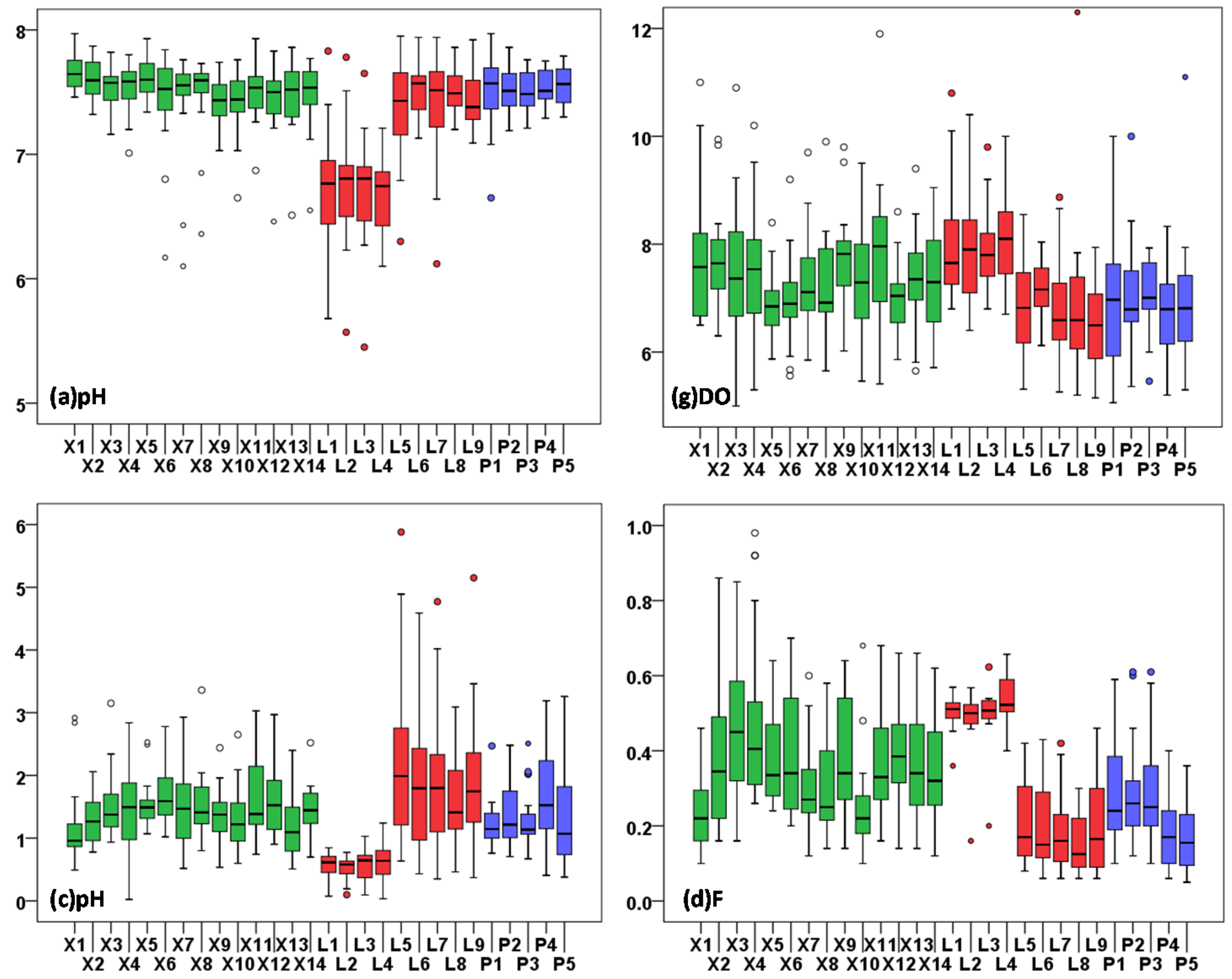
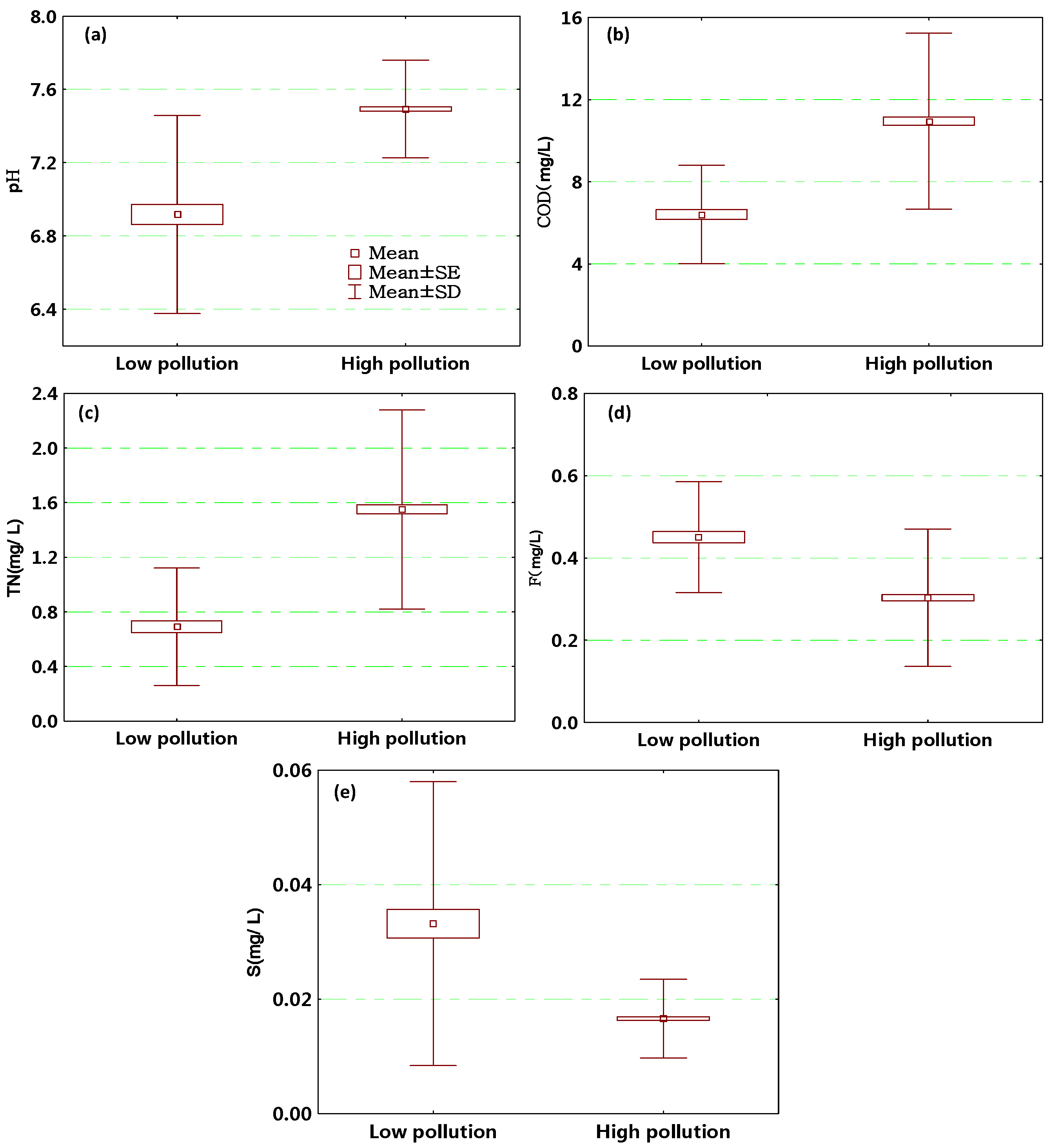
Figure 6 shows the chosen discriminate parameters identified by spatial backward stepwise DA. The pH (
Figure 6a) in low pollution regions was clearly less than in high pollution regions, which was not consistent with analyze results in Danjiangkou Reservoir Basin of China [
41]. It maybe because river segments in this region receives a great deal of acidic mine drainage and waste effluents containing Cu and Zn discharged from the neighboring Dexing Copper Mine and from many smelters and mining/panning activities. The average COD and TN concentration (
Figure 6b,c) in the low pollution region were also clearly less than in the high pollution region. Within high pollution regions, all stations were located in middle to down–stream reaches or near urban areas and therefore in proximity to municipal sewage and industrial waste water. The average F and S concentration (
Figure 6d,e) in low pollution regions were also clearly higher than in high pollution region. Obviously, these excess acidic pollutants were main drivers that leading to lower pH.
Figure 7 preferably illustrates spatial distribution of pH, DO, TN, and F at 27 stations in the east Poyang Lake basin.
Figure 6.
Spatial changes: (a) pH; (b) COD; (c) TN; (d) F and (e) S in the east Poyang Lake basin.
Figure 6.
Spatial changes: (a) pH; (b) COD; (c) TN; (d) F and (e) S in the east Poyang Lake basin.
Figure 7.
Boxplots illustrating distribution of (a) pH; (b) DO (mg/L); (c) TN (mg/L); and (d) F (mg/L) at 27 stations in the east Poyang Lake basin.
Figure 7.
Boxplots illustrating distribution of (a) pH; (b) DO (mg/L); (c) TN (mg/L); and (d) F (mg/L) at 27 stations in the east Poyang Lake basin.
3.3. Data Structure Determination and Source Identification
Based on the normalized log-transformed data sets, PCA/FA was used to further identify the potential pollution sources for the low pollution and high pollution regions. Before the PCA/FA analysis, the Kaiser–Meyer–Olkin (KMO) and Bartlett’s Sphericity tests were carried out on the parameter correlation matrix to examine the validity of PCA/FA. The KMO results for Group 1 and Group 2 were 0.61 and 0.71, respectively, and Bartlett’s Sphericity results were 547.92 and 1611.68 (
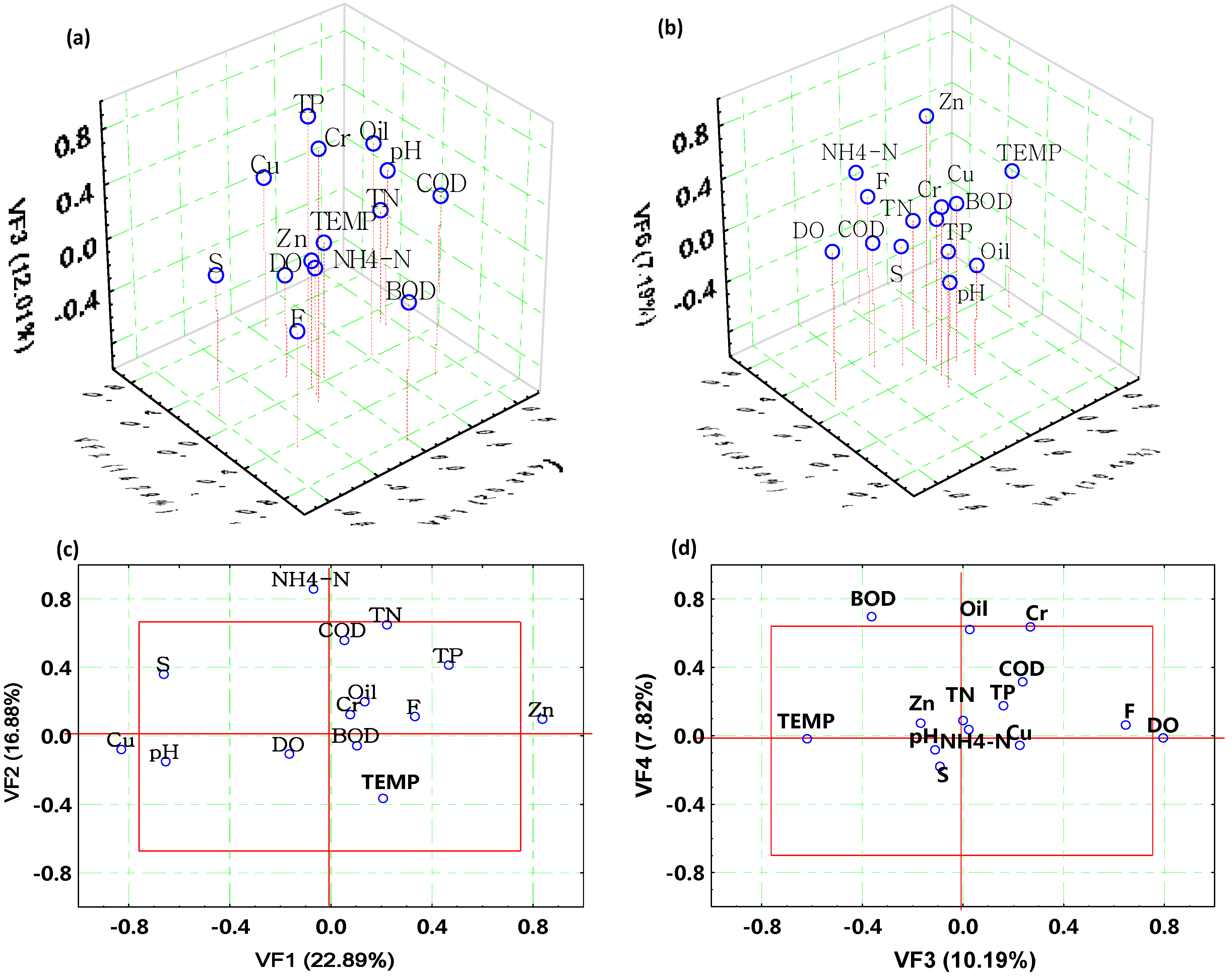
p < 0.05), suggesting that PCA/FA analysis was reasonable to offer significant reductions in dimensionality. Six VFs were calculated for the low pollution region and four VFs for the high pollution region with the eigenvalues great than 1, explaining proximately 78.86% and 57.78% of the total variance in respective surface water quality data sets (
Figure 8 and
Table 6).
Figure 8.
Scatter plot of loadings for the four VFs for group 1 (a and b) and group 2 (c and d).
Figure 8.
Scatter plot of loadings for the four VFs for group 1 (a and b) and group 2 (c and d).
In the low pollution region, among six VFs, VF1, explaining about 25.38% of the total variance, had strong positive loadings of pH and TN and moderate positive loadings of COD, and strong negative loadings of S and moderate negative loadings of F. Generally, high concentrations of total nitrogen reflect agricultural runoff and municipal effluents [
42,
43]; COD is an indicator of organic pollution from industrial and domestic waste water[
44]. The pH is regarded as one of the main reaction conditions for redox reactions involving organic matter, which can regulate the concentration of COD [
45]. Sulphide and fluoride mainly originate from copper mines in this region (e.g., the Dexing Copper Mine in Dexing City), the components of which are very complex for dressing with high sulphur and fluoride [
46]. VF1 included nutrient pollution, organic pollution and mining pollution. VF2 (14.29% of the total variance) had strong positive loadings of Cu and strong negative loadings of BOD, representing metal pollution. VF3, explaining 12.21% of the total variance, had strong positive loadings of Cr and TP and moderate positive loadings of Oil. This factor can be explained as representing influences from point sources, such as copper mines, industrial effluents and domestic wastewater. VF4, accounting for 10.49% of the total variance, had strong positive loadings of temperature and strong negative loadings of dissolved oxygen. The concentration of DO is controlled by temperature and therefore has both a seasonal and a daily cycle [
47]. Therefore, the DO concentration is high in winter and early spring because of low temperature, and is low in summer and fall because of high temperature. VF5 (9.30%) had strong positive loadings on NH
4-N representing non-point source pollution related to agricultural activities. VF6 (7.19%) had strong positive loadings of Zn indicating the metal pollution.
With respect to the data set pertaining to the high pollution region, among four VFs, VF1, explaining about 22.89% of the total variance, had strong positive loadings on Cu and moderate negative loadings on pH and S, basically representing metal pollution from the upstream. VF2 (16.88% of the total variance) had strong positive loadings of NH4-N and moderate positive loading of TN and COD. This factor can be explained as one typical kind of mixed pollution, which consists of point source pollution (e.g., industrial and domestic waste water) and non-point source pollution associated with agricultural activities and atmospheric deposition. VF3, explaining 10.19% of the total variance, had strong positive loadings of DO and moderate positive loadings of F and moderate negative loadings of TEMP. Generally, fluoride is from cement plants, fluorine chemical factories, and copper smelters in this region. The relationship between DO and temperature is explained in the same way as the explanation of VF4 in the low pollution region. VF4 (7.82%) had strong positive loadings of BOD and moderate positive loadings of Oil and Cr. The high concentration of BOD and Oil could represent organic pollution and oil pollution, and Cr is likely from cement plants and copper smelters in this region.
Based on the above analysis, five latent pollutants including nutrients, organics, chemicals, heavy metals and natural pollutants were identified in the study area. Firstly, nutrient pollution (ammonia nitrogen and total nitrogen) was mainly from non-point sources related to agricultural activities and atmospheric deposition and point sources including municipal effluents and fertilizer plant wastewater. In addition, organic pollution (BOD and COD) was usually from point sources (e.g., industrial and domestic waste water). Thirdly, chemical pollution was mainly from the petroleum industry (oil pollution) and copper mines and plating (S and F pollution). Fourthly, heavy metal pollution (Cu, Cr and Zn) was mainly from copper mines and plating. Finally, natural pollution was badly affected by meteorological variations such as the variation of water temperature and dissolved oxygen. Considering the types of pollution in the two regions (
Table 6 and
Figure 6), heavy metals (Cu, Cr and Zn), fluoride and sulfide stood out. Field investigations showed there are many copper mines in the Eastern Poyang Lake Basin, such as the Dexing Copper Mine, which are associated with mineral effluents including fluoride and sulfide.


