
Research on Energy-Saving Production Scheduling Based on a Clustering Algorithm for a Forging Enterprise


Abstract
:1. Introduction
2. Production Investigation and Analysis of DVR Enterprise

| Department | Component | Functions |
|---|---|---|
| Production department | Forging workshop | Forging production, post-forging heat treatment, mold manufacturing and management… |
| Production department | Machining workshop | Rough machining, secondary machining, mold modification, forgings correction… |
| Production department | Heat treatment workshop | Normalizing, Quenching, tempering hardness test… |
| Production department | Comprehensive workshop | Cutting, product packaging, transferring of semi-finished products, outsourcing, raw materials and finished products management. |
| Service department | equipment maintenance workshop | Equipment management & maintenance |
| Service department | Process department | Prepare process plan |
| Service department | Quality assurance department | Inspection and document preparation |
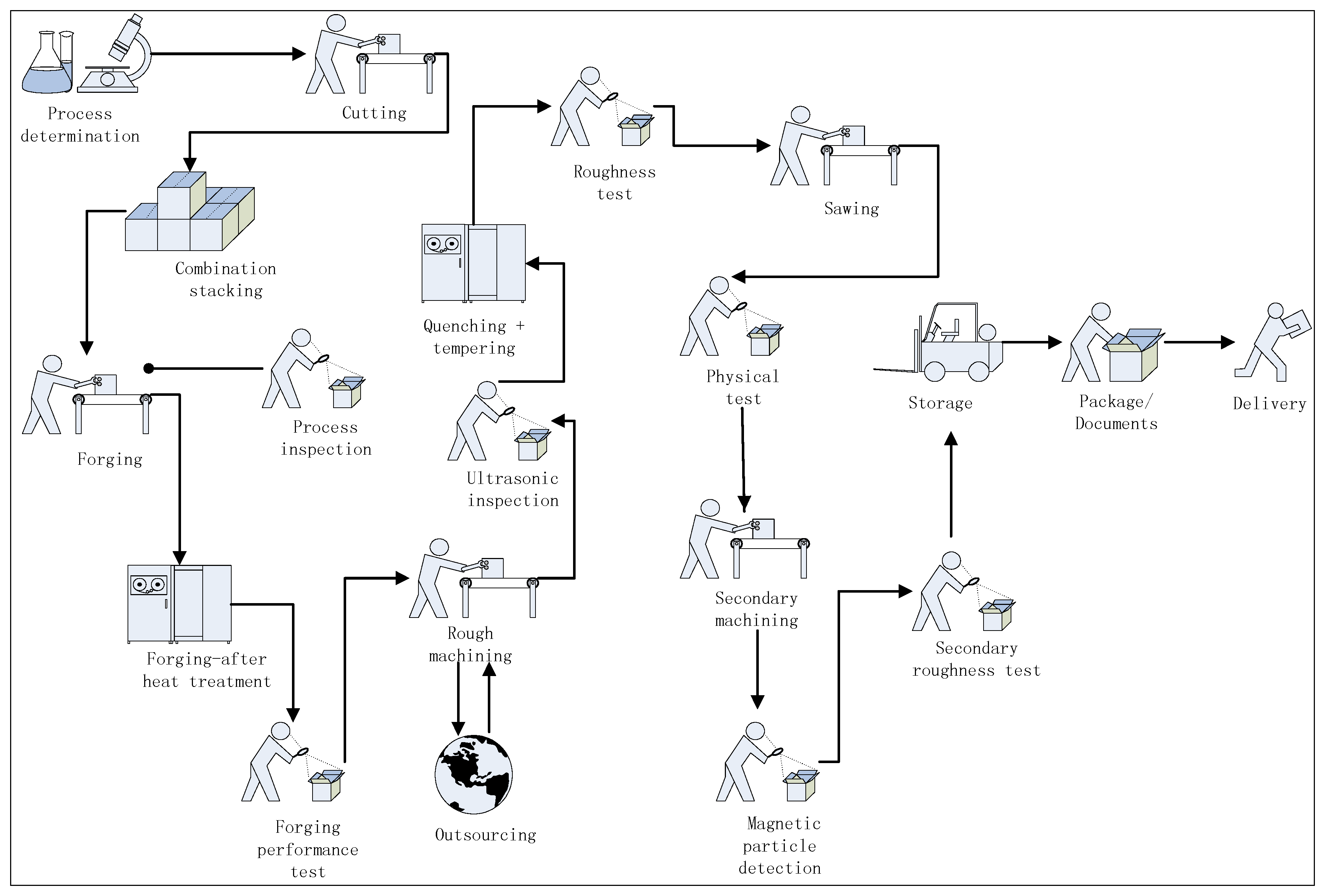
- (1)
- Cutting. Cutting is the start of production and carried out by the sawing machine. Since steel products are widely used in the enterprise, cutting can be primarily used for assessing cost which is normally expressed by material utilization.
- (2)
- Forging. It is a critical procedure for production and also the focus of workshop management. The whole production process is mainly organized according to lead time and quality of forgings. The most important step in forgings’ production is the charging, which means forgings shall be reasonably arranged in a heating furnace and heated up to the initial temperature.
- (3)
- Machining. The machining of forgings is similar to common machining. To ensure individual production and small lot production, universal machine tools are arranged in workshops. Since the machining is not the critical business for a foundry works, the machining is normally outsourced.
- (4)
- Heat treatment. It is usually the final but a critical procedure in production. The heat treatment could comprise normalizing, annealing, solution treatment, quenching and tempering, and the commonly used treatment is thermal refining (quenching + tempering). The key point of heat treatment is similar to forging (how to arrange the heating furnace). However, the principles behind the arrangement vary greatly.
3. Forging Production Scheduling Based on Improved Genetic Algorithm
3.1. Scheduling Problem Description
3.2. Coding
3.3. Population Initialization
3.4. Genetic Operator
- (1)
- Selection
- (2)
- Crossover
- a.
- Extended order crossover operator is adopted as follows:
- b.
- Provided two parent individuals for crossover are A and B. Randomly generate k numbers from steels set N = {1, 2, …, n} to form Γ = (Γ1, Γ2, …, Γk). Amplify Γi 100 times to form Ψ = (Ψ1, Ψ2, …,Ψk) and then select a gene cluster from A to form Z (Z1, Z2, …, Zx) within the interval [Ψ1,Ψ1 + 100].
- c.
- For each gene Zi, select a gene from B within the interval [Ψ1,Ψ1 + 100]. for exchange.
- d.
- As the above, exchange all Zi so as to generate two filial generations.
- a.
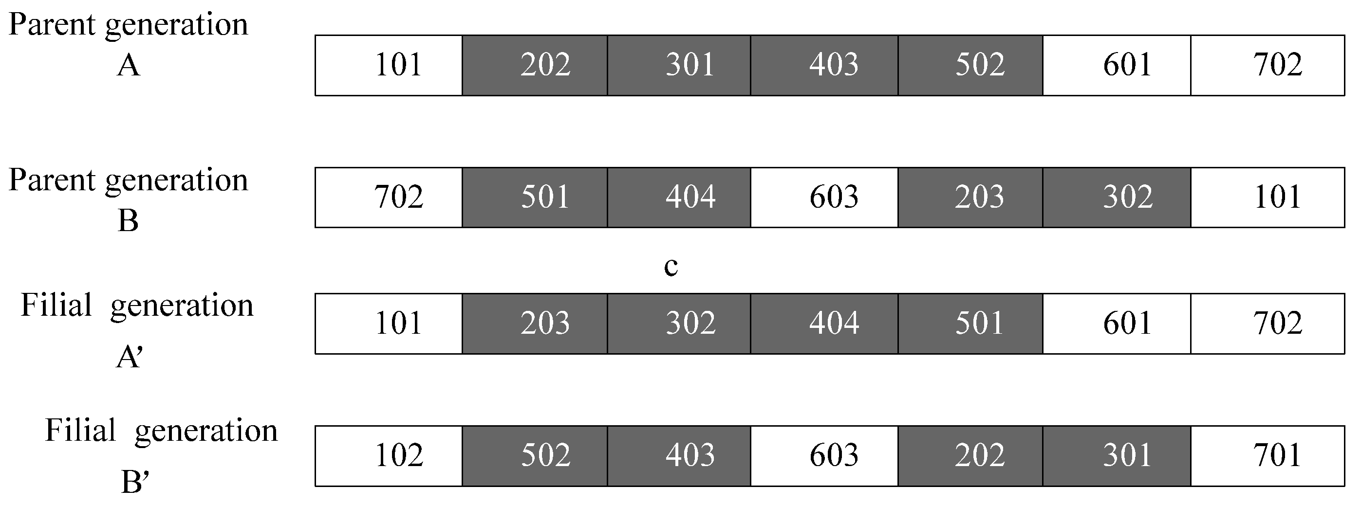
- Randomly generate four numbers 2, 3, 4 and 5 from the aggregate of steels and amplify those numbers 100 times to form Ψ = (200, 300, 400, 500). Then, select genes from parent A within intervals [200,300], [300,400], [400,500] and [500,600], respectively, to form a gene cluster Z = (202, 301, 403, 502) (see the hatched section in Figure 2).
- b.
- For each gene Zi in the cluster (take the gene Zi = {202} as an example), select a gene {203} from B within the interval [200,300] and exchange them.
- c.
- Follow the above method to replace the gene cluster Z = (202, 301, 403, 502) to Z’ = (203, 302, 404, 501) so as to generate two filial generations A’ and B’.
- (3)
- Mutation


3.5. Case Study
| No. | Size | No. | Size |
|---|---|---|---|
| 1 | 12” ingot and 14” ingot | 6 | Φ200 less, □200 less |
| 2 | 17” ingot | 7 | Φ200~Φ300, □200–□300 |
| 3 | 22” ingot | 8 | Φ300~Φ500, □300–□500 |
| 4 | 24” ingot | 9 | Φ500~Φ650, □500–□650 |
| 5 | 26” and bigger ingots | 10 | Φ650~Φ800, □650–□800 |
| No. | 1 | 2 | 3 | 4 | 5 | Delivery Time |
|---|---|---|---|---|---|---|
| 1 | 8.5 | 8.2 | 8.5 | 0 | 0 | 15.5 |
| 2 | 5 | 0 | 0 | 0 | 0 | 12.5 |
| 3 | 7.4 | 7.2 | 0 | 0 | 0 | 10 |
| 4 | 0 | 0 | 0 | 3.4 | 3.6 | 12 |
| 5 | 6 | 5.7 | 0 | 0 | 0 | 4 |
| 6 | 10.7 | 10.2 | 10.3 | 0 | 0 | 18.5 |
| 7 | 0 | 0 | 0 | 4.2 | 4.5 | 20 |
| 8 | 0 | 0 | 5.5 | 5.6 | 5.9 | 8 |
| 9 | 0 | 0 | 4.5 | 4.8 | 4.9 | 14.5 |
| 10 | 5.2 | 5.2 | 0 | 0 | 0 | 17 |
| 11 | 0 | 0 | 5.7 | 5.4 | 5.6 | 5.5 |
| 12 | 0 | 9.7 | 9.4 | 0 | 0 | 13.6 |
| 13 | 4.5 | 4.8 | 4.7 | 0 | 0 | 17 |
| 14 | 5.6 | 5.9 | 0 | 0 | 0 | 7.5 |
| 15 | 0 | 0 | 0 | 3.3 | 3.7 | 20.5 |
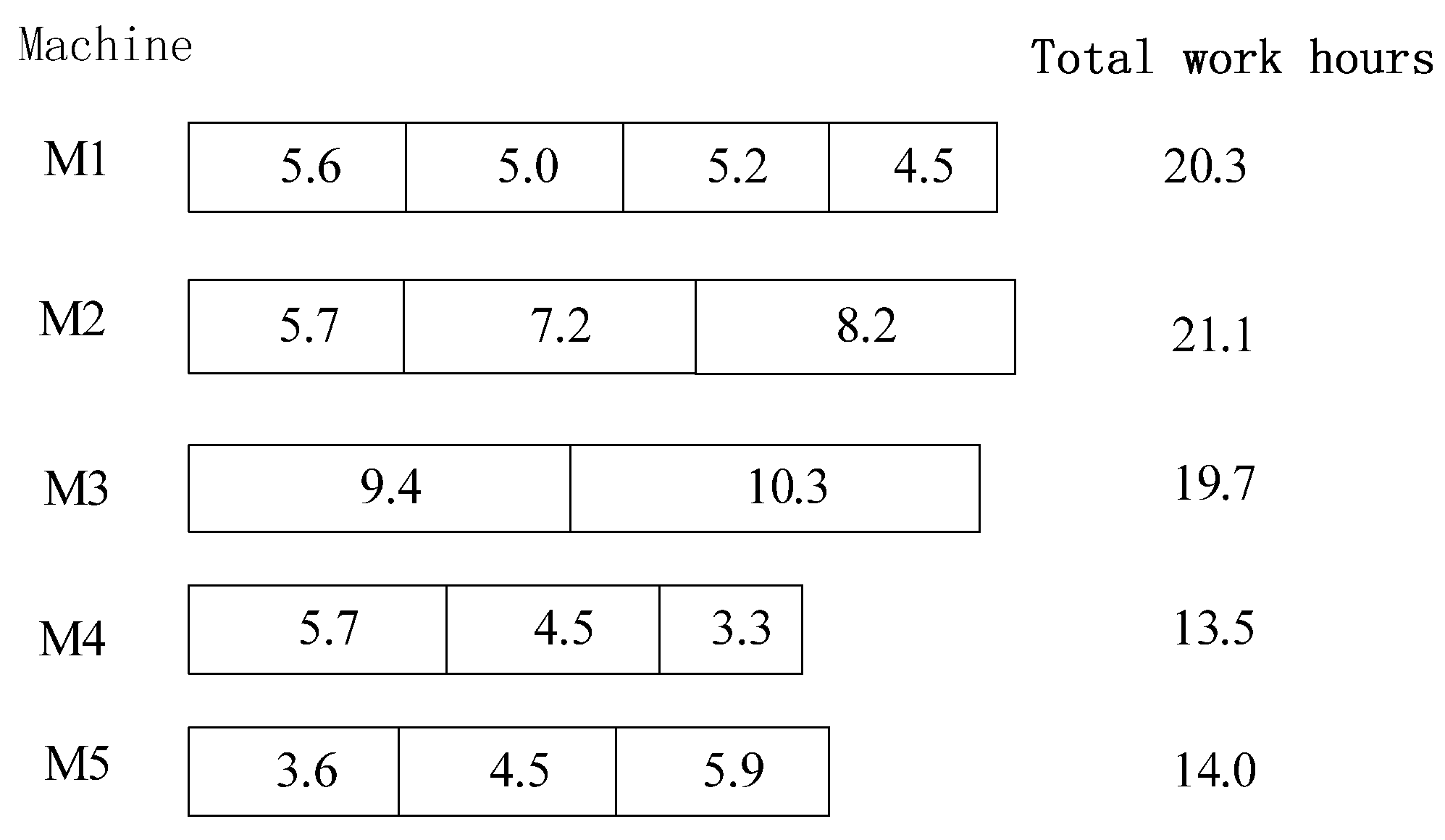
| No. (Machine) | No. (Workpiece) | No. (Machine) | No. (Workpiece) |
|---|---|---|---|
| 1 | 14, 2, 10, 13 | 4 | 11, 9, 15 |
| 2 | 5, 3, 1 | 5 | 4, 7, 8 |
| 3 | 12, 6 |

4. Stacking Combination Optimization for Free Forging
4.1. Stacking Problems Description
- (1)
- The height of piled up material shall not exceed maximum height of furnace. Workpieces shall be stacked within effective heating area.
- (2)
- Workpieces stacked in one furnace should be easily distinguished by weights and specifications. Workpieces with similar specifications shall not be stacked into one furnace. If they have to be stacked into a furnace, label them with marks.
- (3)
- Workpieces with the same material and production batch number shall be stacked into one furnace as far as possible.
- (4)
- Workpieces with different kinds of material can be stacked into one furnace if heating process permits. However, stacking workpieces with the same specification but different kinds of materials shall be strictly prohibited.
- (5)
- Ingot shall be placed around 200 mm away from bottom and wall and at least 200 mm away from other ingots.
- (6)
- Mixing cold ingot with hot ingot is strictly prohibited. Unless otherwise specified, use minimum values for stacking temperature, heating temperature and heating rate (which means to follow the heating regulations for cold ingot).
- (1)
- Maximum stacking coefficient η
- (2)
- Deviation coefficient ε
- (3)
- Deviation ratio ζ
- Classify the material to be forged according to process and specifications. The material classified into a same type can be combined together for heating. A dynamic clustering method is proposed in this paper to realize automatic material classification based on stacking rules.
- For materials which can be combined, optimize the piling up according to the heating process curve, which is fundamental to increasing yield, saving energy for low-carbon production and increasing profit.
4.2. Dynamic Clustering for Forgings
- (1)
- Normalization
- a.
- For indexes where the smaller, the better,
- b.
- For indexes where the bigger, the better,where and xkmax, xkmin represent maximum and minimum of , respectively.
- (2)
- Determination of similarity coefficient
- a.
- Reflexivity. That is .
- b.
- Symmetry. That is .
- c.
- For clustering, the abovementioned matrix R has to be transformed to an equivalent matrix in order to enable transitivity within the matrix [17].
- (3)
- Determination of λ
4.3. Stacking Optimization
4.3.1. Problem Analysis of Stacking Optimization
| Material | Weight or Ingot Size | |
|---|---|---|
| 2400kg or More Octagon Ingot | 2400–1200kg 22” Ingot | |
| 20, 35, 45, Q235 (A3), A105, Q345 16Mn, 16MnD, 30Mn |  |  |
4.3.2. Mathematic Model for Stacking Optimization
- (1)
- Selection of heating furnace
- (2)
- Objective function
- (3)
- Constraints
- (4)
- Optimization
4.4. Case Study
| No. | Forging Tonnage (T)↑ | Initial Temperature (°C)↓ | Weight (kg)↑ | Number of Heat (Times)↓ | Stacking Temperature (°C)↓ |
|---|---|---|---|---|---|
| 1 | 5 | 1100 | 300 | 1 | 1200 |
| 2 | 3 | 1200 | 500 | 1 | 900 |
| 3 | 3 | 1100 | 400 | 1 | 1200 |
| 4 | 5 | 1100 | 500 | 2 | 1200 |
| 5 | 5 | 1100 | 400 | 2 | 900 |
| 6 | 5 | 1200 | 500 | 2 | 1200 |
| 7 | 5 | 1200 | 300 | 2 | 900 |
| 8 | 5 | 1200 | 500 | 1 | 1200 |
| max | 5 | 1200 | 500 | 2 | 1200 |
| min | 3 | 1100 | 300 | 1 | 900 |
- (1)
- After being normalized, we can get
- (2)
- Obtain similar matrix
- (3)
- Forgings classification (clustering)
- (4)
- Stacking optimization
| No. | Unit Ingot Weight (kg) | Quantity |
|---|---|---|
| 1 | 310 | 25 |
| 3 | 518 | 10 |
| 4 | 415 | 15 |
| 5 | 520 | 5 |
| 6 | 309 | 20 |
| 7 | 516 | 26 |
| Furnace No. | Forging No. | Quantity | Gross Weight (T) | Deviation from Theoretical Value (T) | Average Difference f (%) |
|---|---|---|---|---|---|
| 1 | 1 | 25 | 7.75 | 0.25 | 3.23 |
| 2 | 03, 04 | 10, 6 | 7.67 | 0.33 | 4.3 |
| 3 | 04, 05, 06 | 9, 5, 5 | 7.8 | 0.2 | 2.56 |
| 4 | 06, 07 | 15, 2 | 5.667 | 0.333 | 4.26 |
| 5 | 7 | 11 | 5.632 | 0.368 | 6.53 |
| 6 | 7 | 13 | 6.708 | 0.282 | 4.2 |
5. Conclusions
- (1)
- The presented work focuses on two types of scheduling for a forging enterprise. One is for cutting and machining scheduling, which is similar to traditional machining scheduling, and the other is for forging and heat treatment scheduling, characterized by stacking and heat treatment.
- (2)
- Dynamic clustering is proposed for forging combination before stacking optimization. The forgings to be optimized are clustered according to certain rules, which can greatly reduce the computations required in stacking optimization in order to more easily obtain a solution.
- (3)
- In reality, the production manager judges different forgings based on empirical criteria. This empirical standard is generally difficult to portray. In the fuzzy clustering analysis, λ (0 < λ < 1) is utilized to indicate the empirical criteria. The clustering results vary with λ, resulting in various heating plans with different production efficiency, energy consumption and carbon emissions.
- (4)
- The proposed stacking optimization involves ensuring the gross weight of forgings is as close to the maximum batch capacity as possible.
Acknowledgments
Author Contributions
Conflicts of Interest
References
- Park, C.W.; Kwon, K.S.; Kim, W.B.; Min, B.K.; Park, S.J.; Sung, I.H. Energy consumption reduction technology in manufacturing—A selective review of policies, standards, and research. Int. J. Precis. Eng. Manuf. 2009, 10, 151–173. [Google Scholar] [CrossRef]
- Ngai, E.W.T.; Ng, C.T.D.; Huang, G. Energy Sustainability for Production Design and Operations. Int. J. Prod. Econ. 2013, 146, 383–385. [Google Scholar] [CrossRef]
- Deif, A.M. A system model for green manufacturing. J. Clean. Prod. 2011, 19, 1553–1559. [Google Scholar] [CrossRef]
- Vijayaraghavan, A.; Helu, M. Enabling Technologies for Assuring Green Manufacturing. In Green Manufacturing; Dornfeld, D.A., Ed.; Springer: New York, NY, USA, 2013; pp. 255–267. [Google Scholar]
- Chuang, S.P.; Yang, C.L. Key success factors when implementing a green-manufacturing system. Prod. Plann. Contr. 2014, 25, 923–937. [Google Scholar] [CrossRef]
- Reich-Weiser, C.; Simon, R.; Fleschutz, T.; Yuan, C.; Vijayaraghavan, A.; Onsrud, H. Metrics for Green Manufacturing. In Green Manufacturing; Dornfeld, D.A., Ed.; Springer: New York, NY, USA, 2013; pp. 49–81. [Google Scholar]
- Linke, B.; Huang, Y.C.; Dornfeld, D. Establishing greener products and manufacturing processes. Int. J. Precis. Eng. Manuf. 2012, 13, 1029–1036. [Google Scholar] [CrossRef]
- Bhattacharya, A.; Mohapatra, P.; Kumar, V.; Dey, P.K.; Brady, M.; Tiwari, M.K. Green supply chain performance measurement using fuzzy ANP-based balanced scorecard: A collaborative decision-making approach. Prod. Plann. Contr. Manage. Oper. 2014, 25, 698–714. [Google Scholar] [CrossRef]
- He, Y.; Liu, F. Methods for integrating energy consumption and environmental impact considerations into the production operation of machining processes. Chinese J. Mech. Eng. 2010, 2, 428–435. [Google Scholar] [CrossRef]
- Domingo, R.; Aguado, S. Overall Environmental Equipment Effectiveness as a Metric of a Lean and Green Manufacturing System. Sustainability 2015, 7, 9031–9047. [Google Scholar] [CrossRef]
- Edenhofer, O.; Seyboth, K. Intergovernmental panel on climate change. In Encyclopedia of Energy Natural Resource, and Environmental Economics; Shogren, J.F., Ed.; Elsevier Inc.: Philadelphia, PA, USA, 2013; Volume 1, pp. 48–56. [Google Scholar]
- Tsai, W.T. An analysis of shifting to a low-carbon society through energy policies and promotion measures in Taiwan. Energ. Sourc. B Energ. Econ. Plann. 2014, 9, 391–397. [Google Scholar] [CrossRef]
- Fang, K.; Uhan, N.; Zhao, F.; Sutherland, J.W. A new approach to scheduling in manufacturing for power consumption and carbon footprint reduction. J. Manuf. Syst. 2011, 30, 234–240. [Google Scholar] [CrossRef]
- Dai, M.; Tang, D.; Giret, A.; Salido, M.A.; Li, W.D. Energy-efficient scheduling for a flexible flow shop using an improved genetic-simulated annealing algorithm. Robot. Comput. Integrated. Manuf. 2013, 29, 418–429. [Google Scholar] [CrossRef]
- Wicaksono, H.; Belzner, T.; Ovtcharova, J. Efficient energy performance indicators for different level of production organizations in manufacturing companies. In Advances in Production Management Systems. Sustainable Production and Service Supply Chains; Springer: Berlin, Germany, 2013; pp. 249–256. [Google Scholar]
- Chang, P.C.; Huang, W.H.; Wu, J.L.; Cheng, T.C.E. A block mining and re-combination enhanced genetic algorithm for the permutation flowshop scheduling problem. Int. J. Prod. Econ. 2013, 141, 45–55. [Google Scholar] [CrossRef]
- Tian, Y.; Wang, T.Y.; He, G.Y.; Ding, B.H. Disassembly Sequence Planning Based on Generalized Axis Theory. J. Mech. Eng. 2009, 45, 160–170. [Google Scholar] [CrossRef]
- Chan, K.; Gibbons, A.; Pias, M.; Rytter, W. On the PVM computations of transitive closure and algebraic path problems. In Recent Advances in Parallel Virtual Machine and Message Passing Interface; Springer: Berlin, Germany, 1988; pp. 338–345. [Google Scholar]
- Zhang, D.S.; Chao, J.I.; Zheng, W.K. Method of Examination Analysis Based on Fuzzy Cluster. Comput. Knowl. Technol. 2009, 33, 9579–9580, 9590. [Google Scholar]
© 2016 by the authors; licensee MDPI, Basel, Switzerland. This article is an open access article distributed under the terms and conditions of the Creative Commons by Attribution (CC-BY) license (http://creativecommons.org/licenses/by/4.0/).
Share and Cite
Tong, Y.; Li, J.; Li, S.; Li, D. Research on Energy-Saving Production Scheduling Based on a Clustering Algorithm for a Forging Enterprise. Sustainability 2016, 8, 136. https://doi.org/10.3390/su8020136
Tong Y, Li J, Li S, Li D. Research on Energy-Saving Production Scheduling Based on a Clustering Algorithm for a Forging Enterprise. Sustainability. 2016; 8(2):136. https://doi.org/10.3390/su8020136
Chicago/Turabian StyleTong, Yifei, Jingwei Li, Shai Li, and Dongbo Li. 2016. "Research on Energy-Saving Production Scheduling Based on a Clustering Algorithm for a Forging Enterprise" Sustainability 8, no. 2: 136. https://doi.org/10.3390/su8020136