
Vegetation Carbon Storage, Spatial Patterns and Response to Altitude in Lancang River Basin, Southwest China

 , ,
, ,
Abstract
:1. Introduction
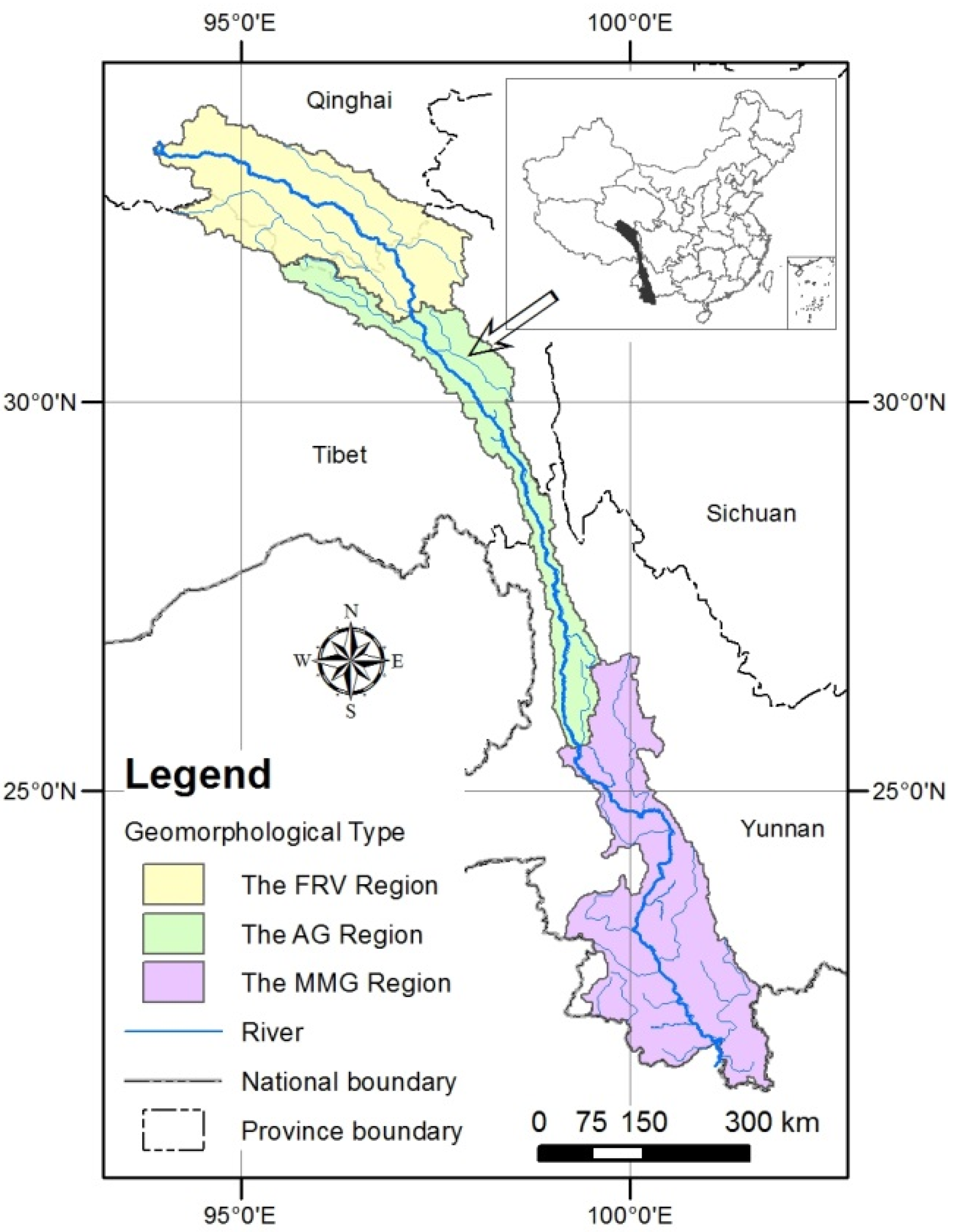
2. Study Area
3. Methods
3.1. Data Collection
3.2. Estimation of Vegetation C Storage

| Forest Type | a | b | n | R |
|---|---|---|---|---|
| Abies and Picea | 0.3809 | 62.8917 | 122 | 0.9123 |
| Cypress | 0.5137 | 31.0518 | 12 | 0.9855 |
| Evergreen and deciduous broadleaf mixed forest | 0.6011 | 97.3843 | 9 | 0.8287 |
| Pinus armandii, P. densata | 0.4758 | 26.6772 | 31 | 0.9594 |
| Larix | 0.6433 | 6.8686 | 22 | 0.9619 |
| P. massoniana | 0.6404 | 7.3645 | 14 | 0.9995 |
| Tropical rain forest, monsoon forest | 1.1243 | 18.5632 | 12 | 0.9946 |
| Mountainous poplar-birth forest | 0.5671 | 48.0016 | 21 | 0.8641 |
| Cunninghamia lanceolata | 0.4634 | 30.3323 | 36 | 0.8344 |
| Subtropical evergreen broadleaf forest | 0.8879 | 29.0708 | 158 | 0.9366 |
| Evergreen sclerophyllous broadleaf oaks | 0.5363 | 84.7126 | 9 | 0.9254 |
| P. Yunnanensis, P. kesiya var. langbianensis | 0.7685 | 1.5945 | 44 | 0.9955 |
| Alnus | 1.0054 | 4.4856 | 10 | 0.9994 |
| * Betula | 1.0687 | 10.2370 | 9 | 0.9770 |
| * Eucalyptus | 0.8873 | 4.5539 | 20 | 1.0000 |
| * Lucidophyllous forests | 1.0357 | 8.0591 | 17 | 0.9100 |
| * Tsuga, Cryptomeria | 0.4158 | 41.3318 | 21 | 0.9400 |
| * Populus | 0.4754 | 30.6034 | 10 | 0.9290 |
3.3. Data Analysis
4. Results
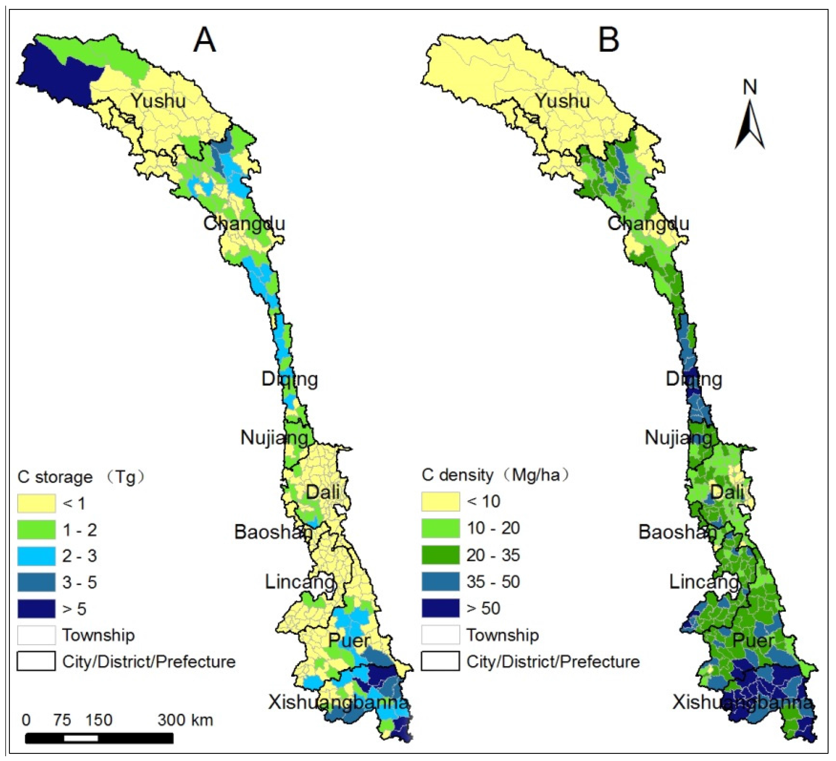
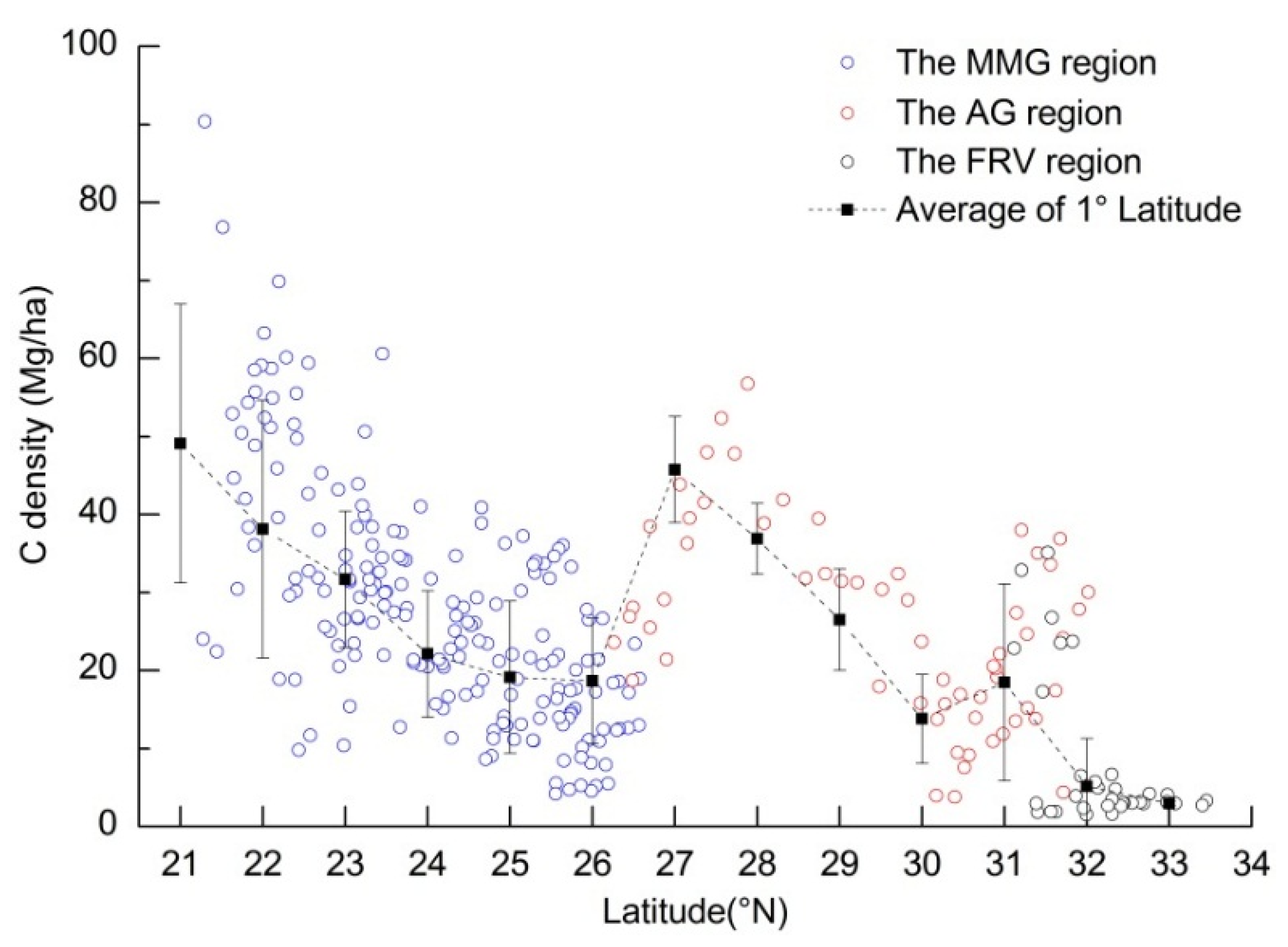
4.1. Spatial Distribution and Latitudinal Patterns of Vegetation C Storage along the LRB
4.2. C Storage of Vegetation Types and Dominant Tree Species
| Vegetation Type | C Storage Tg | C Density Mg/ha | |
|---|---|---|---|
| Forest | Arbor | 238.64 | 47.95 |
| Shrub | 23.81 | 12.97 | |
| Economic forest | 10.64 | 19.86 | |
| Bamboo | 3.17 | 64.57 | |
| Subtotal | 276.27 | 37.09 | |
| Grassland | 21.10 | 2.92 | |
| Desert | 0.09 | 0.09 | |
| Swamp | 2.40 | 18.00 | |
| Tree Species | C Storage Tg | C Density Mg/hm2 | Distribution Region | Tree Species | C Storage Tg | C Density Mg/hm2 | Distribution Region |
|---|---|---|---|---|---|---|---|
| Larix | 0.16 | 42.97 | AG | Betula | 0.66 | 33.41 | AG, MMG |
| P. densata | 0.40 | 33.32 | AG | Eucalyptus | 0.25 | 4.47 | MMG |
| Abies | 6.92 | 60.52 | AG | Populus | 0.15 | 31.56 | AG, MMG |
| Picea | 2.09 | 62.37 | AG | Castanopsis | 0.79 | 35.49 | MMG |
| P. armandii | 0.61 | 30.61 | AG, MMG | Alnus | 1.80 | 31.57 | AG, MMG |
| Cypress | 0.17 | 21.21 | AG, MMG | Schima | 0.16 | 26.85 | MMG |
| C. lanceolata | 0.17 | 22.40 | MMG | Cassia siamea | 0.02 | 25.67 | MMG |
| Tsuga | 0.59 | 50.83 | AG, MMG | Anthocephalus chinensis | 0.02 | 21.48 | MMG |
| P. Yunnanensis | 7.82 | 26.60 | MMG | Tectona grandis | 0.03 | 37.57 | MMG |
| P. kesiya var. langbianensis | 23.95 | 31.32 | MMG | Hevea | 9.34 | 22.57 | MMG |
| Oaks | 55.23 | 63.26 | FRV, AG, MMG | Sabina tibetica | 0.18 | 20.97 | FRV |
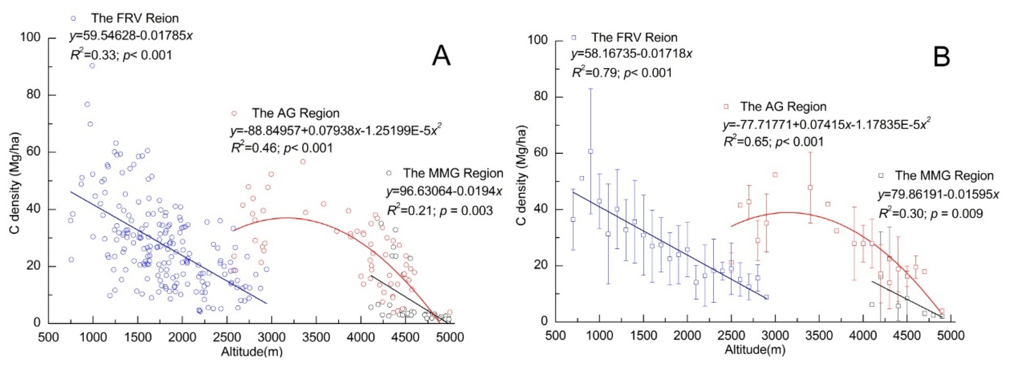
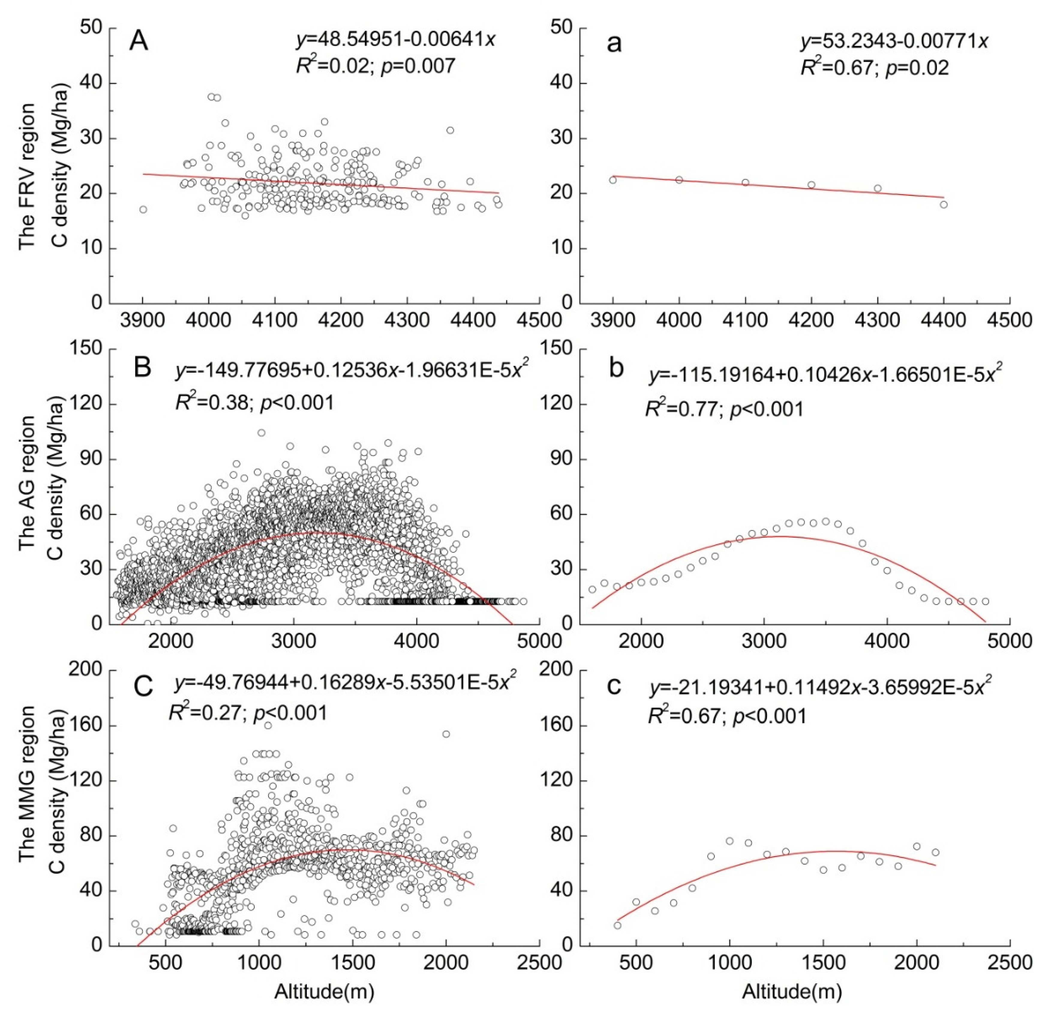
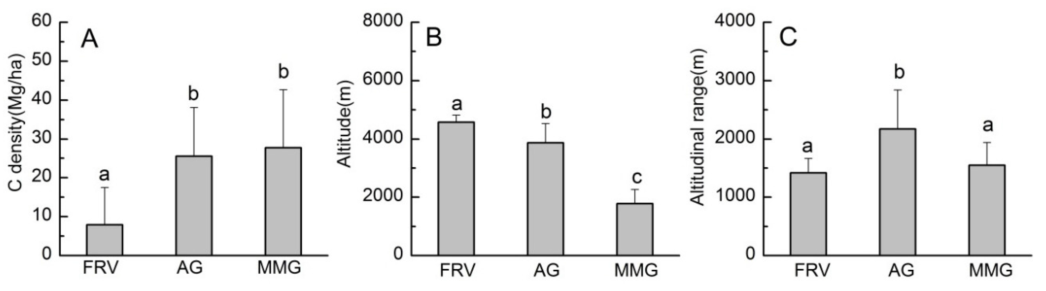
4.3. Altitudinal Patterns of C Storage in Three Geomorphological Regions


5. Discussion
5.1. Error Analysis of the Accuracy of C Storage
5.2. Influencing Mechanism for C Storage by Altitude
5.3. Tradeoff between C Storage and Local Development
6. Conclusions
Acknowledgments
Author Contributions
Conflicts of Interest
Appendix A
| Province/Autonomous Region | Prefecture/City/District | County | Number of Towns | Area 104 ha | C Storage Tg | C Density Mg/ha | Area Percentage % | C Storage Percentage % |
|---|---|---|---|---|---|---|---|---|
| Qinghai | Yushu | Nangqian | 10 | 120.70 | 4.94 | 4.09 | 7.59 | 1.64 |
| Yushu | 3 | 70.71 | 2.52 | 3.56 | 4.45 | 0.84 | ||
| Zaduo | 8 | 356.55 | 12.25 | 3.43 | 22.42 | 4.08 | ||
| Subtotal | 21 | 547.96 | 19.70 | 3.60 | 34.46 | 6.56 | ||
| Tibet | Chaya | 13 | 79.79 | 10.61 | 13.30 | 5.02 | 3.53 | |
| Changdu | Changdu | 15 | 104.39 | 25.81 | 24.72 | 6.57 | 8.59 | |
| Dingqing | 8 | 30.86 | 0.51 | 1.65 | 1.94 | 0.17 | ||
| Gongjue | 4 | 3.96 | 0.14 | 3.60 | 0.25 | 0.05 | ||
| Jiangda | 5 | 32.85 | 1.61 | 4.91 | 2.07 | 0.54 | ||
| Leiwuqi | 10 | 57.52 | 11.06 | 19.23 | 3.62 | 3.68 | ||
| Mangkang | 11 | 47.61 | 11.71 | 24.60 | 2.99 | 3.90 | ||
| Zuogong | 6 | 15.53 | 3.72 | 23.98 | 0.98 | 1.24 | ||
| Naqu | Baqing | 1 | 16.46 | 0.43 | 2.61 | 1.04 | 0.14 | |
| Subtotal | 73 | 388.97 | 65.61 | 16.87 | 24.46 | 21.85 | ||
| Yunnan | Baoshan | Changning | 8 | 13.49 | 2.00 | 14.82 | 0.85 | 0.67 |
| Longyang | 3 | 3.75 | 0.91 | 24.18 | 0.24 | 0.30 | ||
| Dali | Dali | 11 | 7.64 | 0.81 | 10.64 | 0.48 | 0.27 | |
| Eryuan | 12 | 21.07 | 2.77 | 13.17 | 1.33 | 0.92 | ||
| Heqing | 1 | 1.92 | 0.20 | 10.17 | 0.12 | 0.07 | ||
| Jianchuan | 7 | 17.58 | 2.82 | 16.02 | 1.11 | 0.94 | ||
| Nanjian | 6 | 9.04 | 1.04 | 11.45 | 0.57 | 0.34 | ||
| Weishan | 8 | 21.30 | 2.70 | 12.65 | 1.34 | 0.90 | ||
| Yangbi | 11 | 13.95 | 2.18 | 15.62 | 0.88 | 0.73 | ||
| Yongping | 8 | 32.62 | 11.22 | 34.40 | 2.05 | 3.74 | ||
| Yunlong | 10 | 36.22 | 7.41 | 20.46 | 2.28 | 2.47 | ||
| Diqing | Deqin | 4 | 21.37 | 8.17 | 38.23 | 1.34 | 2.72 | |
| Weixi | 8 | 29.41 | 13.57 | 46.13 | 1.85 | 4.52 | ||
| Lincang | Cangyuan | 7 | 10.11 | 3.59 | 35.52 | 0.64 | 1.20 | |
| Fengqing | 13 | 14.74 | 3.81 | 25.84 | 0.93 | 1.27 | ||
| Gengma | 4 | 9.35 | 3.60 | 38.47 | 0.59 | 1.20 | ||
| Linxiang | 5 | 6.16 | 2.01 | 32.64 | 0.39 | 0.67 | ||
| Shuangjiang | 6 | 14.61 | 4.65 | 31.83 | 0.92 | 1.55 | ||
| Yongde | 1 | 1.40 | 0.29 | 20.44 | 0.09 | 0.10 | ||
| Yunxian | 11 | 18.87 | 4.84 | 25.62 | 1.19 | 1.61 | ||
| Nujiang | Lanping | 8 | 35.49 | 9.06 | 25.52 | 2.23 | 3.02 | |
| Pu'er | Jiangcheng | 1 | 7.26 | 0.85 | 11.69 | 0.46 | 0.28 | |
| Jingdong | 5 | 12.00 | 2.21 | 18.44 | 0.75 | 0.74 | ||
| Jinggu | 11 | 52.59 | 16.76 | 31.87 | 3.31 | 5.58 | ||
| Lancang | 19 | 51.73 | 18.87 | 36.49 | 3.25 | 6.28 | ||
| Menglian | 4 | 4.89 | 0.91 | 18.58 | 0.31 | 0.30 | ||
| Ning'er | 4 | 11.80 | 2.00 | 16.96 | 0.74 | 0.67 | ||
| Simao | 4 | 16.97 | 6.57 | 38.72 | 1.07 | 2.19 | ||
| Zhenyuan | 5 | 14.64 | 2.78 | 19.00 | 0.92 | 0.93 | ||
| Xishuangbanna | Jinghong | 8 | 58.24 | 31.17 | 53.51 | 3.66 | 10.38 | |
| Menghai | 10 | 22.56 | 12.52 | 55.49 | 1.42 | 4.17 | ||
| Mengla | 9 | 60.33 | 32.75 | 54.28 | 3.79 | 10.90 | ||
| Subtotal | 232 | 653.11 | 215.01 | 32.92 | 41.08 | 71.59 | ||
| Total | 326 | 1590.04 | 300.32 | 18.89 | 100.00 | 100.00 | ||
References
- Piao, S.L.; Fang, J.; Huang, Y. The carbon balance of terrestrial ecosystems in China. China Basic Sci. 2010, 12, 20–22. [Google Scholar] [CrossRef] [PubMed]
- Dixon, R.K.; Solomon, A.M.; Brown, S.; Houghton, R.A.; Trexier, M.C.; Wisniewski, J. Carbon pools and flux of global forest ecosystem. Science 1994, 263, 185–190. [Google Scholar] [CrossRef] [PubMed]
- Scurlock, J.M.O.; Cramer, W.; Olson, R.J.; Parton, W.J.; Prince, S.D. Terrestrial NPP: Towards a consistent data set for global model evaluation. Ecol. Appl. 1999, 9, 913–919. [Google Scholar] [CrossRef]
- Hu, H.; Wang, G. Changes in forest biomass carbon storage in the South Carolina Piedmont between 1936 and 2005. Forest Ecol. Manag. 2008, 255, 1400–1408. [Google Scholar] [CrossRef]
- Pan, Y.D.; Birdsey, R.A.; Fang, J.; Houghton, R.; Kauppi, P.E.; Kurz, W.A.; Phillips, O.L.; Shvidenko, A.; Lewis, S.L.; Canadell, J.G.; et al. A large and persistent carbon sink in the world’s forests. Science 2011, 333, 988–993. [Google Scholar] [CrossRef] [PubMed]
- Guo, Z.D.; Hu, H.; Li, P.; Li, N.; Fang, J. Spatio-temporal changes in biomass carbon sinks in China’s forests during 1977–2008. Sci. China Life Sci. 2013, 56, 661–671. [Google Scholar] [CrossRef] [PubMed]
- Hu, H.F.; Wang, S.; Guo, Z.; Xu, B.; Fang, J. The stage-classified matrix models project a significant increase in biomass carbon stocks in China's forests between 2005 and 2050. Sci. Rep. 2015, 5, 11203. [Google Scholar] [CrossRef] [PubMed]
- Fang, J.Y.; Huang, Y.; Zhu, J.; Sun, W.; Hu, H. Carbon budget of forest ecosystems and its driving forces. China Basic Sci. 2015, 3, 20–25. [Google Scholar]
- Zha, T.G.; Zhang, Z.; Zhu, J.; Cui, L.; Zhang, J.; Chen, J.; Tan, J.; Fang, X. Carbon storage and carbon cycle in forest ecosystem. Sci. Soil Water Conserv. 2008, 6, 112–119. [Google Scholar]
- Song, C.; Woodcock, C.E. A regional forest ecosystem carbon budget model: Impacts of forest age structure and landuse history. Ecol. Model. 2003, 164, 33–47. [Google Scholar] [CrossRef]
- Nave, L.E.; Vance, E.D.; Swanston, C.W.; Curtis, P.S. Harvest impacts on soil carbon storage in temperate forests. For. Ecol. Manag. 2010, 259, 857–866. [Google Scholar] [CrossRef]
- Stegen, J.C.; Swenson, N.G.; Enquist, B.J.; White, E.P.; Phillips, O.L.; Jørgensen, P.M.; Weiser, M.D.; Mendoza, A.M.; Vargas, P.N. Variation in above-ground forest biomass across broad climatic gradients. Glob. Ecol. Biogeogr. 2011, 20, 744–754. [Google Scholar] [CrossRef]
- Liu, Y.; Sun, X.; Fan, J.; Zhang, J. Carbon storage and its dynamics of forest vegetations in Liaoning Province. Ecol. Environ. Sci. 2015, 24, 211–216. [Google Scholar]
- Huang, L.; Shao, Q.; Liu, J. The spatial and temporal patterns of carbon sequestration by forestation in Jiangxi Provinc. Acta Ecol. Sin. 2015, 35, 2105–2118. [Google Scholar]
- De Castilho, C.V.; Magnusson, W.E.; de Araújo RN, O.; Luizao, R.C.; Luizao, F.J.; Lima, A.P.; Higuchi, N. Variation in aboveground tree live biomass in a central Amazonian Forest: Effects of soil and topography. For. Ecol. Manag. 2006, 234, 85–96. [Google Scholar] [CrossRef]
- Xiao, Y.; An, K.; Yang, Y.; Xie, G.; Lu, C. Forest carbon storage trends along altitudinal gradients in Beijing, China. J. Resour. Ecol. 2014, 5, 148–156. [Google Scholar]
- Djukic, I.; Zehetner, F.; Tatzber, M.; Gerzabek, M.H. Soil organic-matter stocks and characteristics along an Alpine elevation gradient. J. Plant Nutr. Soil Sci. 2010, 173, 30–38. [Google Scholar] [CrossRef]
- Takeuchi, T.; Kobayashi, T.; Nashimoto, M. Altitudinal differences in bark stripping by sika deer in the subalpine coniferous forest of Mt. Fuji. Forest Ecol. Manag. 2011, 261, 2089–2095. [Google Scholar] [CrossRef]
- Fang, J.Y.; Chen, A. Dynamic forest biomass carbon pools in China and their significance. Acta Bot. Sin. 2001, 43, 967–973. [Google Scholar]
- He, D.M.; Tang, Q. China International Rivers; Science Press: Beijing, China, 2000; pp. 1–209. [Google Scholar]
- He, D.M.; Feng, Y.; Hu, J. Utilization of Water Resources and Environmental Conservation in the International Rivers, Southwest China; Science Press: Beijing, China, 2007; pp. 1–225. [Google Scholar]
- Wang, J.; Cui, B.; Yao, H. Spatio-temporal dynamic study on landscape patterns in Lancang River watershed of Yunnan province. J. Soil Water Conserv. 2007, 21, 85–97. [Google Scholar]
- Qiu, G.X. Research on Environmental Planning of Lancang River Basin in Yunnan Province; Yunnan Environmental Science Press: Kunming, China, 1996; pp. 1–10. [Google Scholar]
- Luo, T.X. Patterns of Net Primary Productivity for Chinese Major Forest Types and Their Mathematical Models. Ph.D. Thesis, The Commission for Integrated Survey of Natural Resources, Chinese Academy of Sciences, Beijing, China, 1996. [Google Scholar]
- Fu, H.; Chen, A. Accumulation of above-ground biomass and nutrients in swidden fallows: A comparison between planted alder fallows and unmanaged grassy fallows in Yunnan. Acta Ecol. Sin. 2004, 24, 209–214. [Google Scholar]
- Department of Animal Product of Ministry of Agriculture of China. China Grassland Resource Data; China Agriculture Scientech Press: Beijing, China, 1994; pp. 1–366. [Google Scholar]
- Crutzen, P.J.; Andreae, M.O. Biomass burning in the tropics: Impact on the atmospheric chemistry and biogeochemical cycles. Science 1990, 250, 1669–1678. [Google Scholar] [CrossRef] [PubMed]
- Fang, J.Y.; Chen, A.; Peng, C.; Zhao, S.; Ci, L. Changes in forest biomass carbon storage in China between 1949 and 1998. Science 2001, 292, 2320–2322. [Google Scholar] [CrossRef] [PubMed]
- Fang, J.Y.; Guo, Z.; Piao, S.; Chen, A. Terrestrial vegetation carbon sinks in China, 1981–2000. Sci. China Earth Sci. 2007, 37, 804–812. [Google Scholar] [CrossRef]
- Liu, Y.C.; Yu, G.; Wang, Q.; Zhang, Y.; Xu, Z. Carbon carry capacity and carbon sequestration potential in China based on an integrated analysis of mature forest biomass. Sci. China Life Sci. 2014, 57, 1218–1229. [Google Scholar] [CrossRef] [PubMed]
- Yang, F.; Huang, L.; Shao, Q.; Bao, Y. Forest carbon storage and its sequestration potential in the southeast of Guizhou Province during 1990–2050. J. Geo-Inf. Sci. 2015, 17, 309–316. [Google Scholar]
- Fang, J.Y.; Chen, A.; Zhao, S.; Ci, L. Estimating biomass carbon of China’s forests: Supplementary notes on report published in science (291:2320–2322) by Fang et al. (2001). Acta Phytoecol. Sin. 2002, 26, 243–249. [Google Scholar]
- Fang, J.Y.; Liu, G.; Xu, S. Carbon cycling in terrestrial ecosystems in China, In Studies on Emissions and Their Mechanisms of Greenhouse Gases in China; Wang, G.C., Wen, Y., Eds.; China Environmental Science Press: Beijing, China, 1996; pp. 81–149. [Google Scholar]
- Tang, J.W.; Pang, J.; Chen, M.; Guo, X.; Zeng, R. Biomass and its estimation model of rubber plantations in Xishuangbanna, Southwest China. Chin. J. Ecol. 2009, 28, 1942–1948. [Google Scholar]
- You, X.Q. Requirement on Nutrient and Accumulation on Biomass by up-Ground Parts of Tea Plants under Field Conditions. Master’s Thesis, Tea Research Institute, Chinese Academy of Agricultural Sciences, Hangzhou, China, 2008. [Google Scholar]
- Nie, D.P. Structural dynamics of bamboo forest stands. Sci. Silv. Sin. 1994, 30, 201–208. [Google Scholar]
- Piao, S.L.; Fang, J.; He, J.; Xiao, Y. Spatial Distribution of Grassland Biomass in China. Acta Phytoecol. Sin. 2004, 28, 491–498. [Google Scholar]
- Pacala, S.W.; Hurtt, G.C.; Baker, D.; Peylin, P.; Houghton, R.A.; Birdsey, R.A.; Heath, L.; Sundquist, E.T.; Stallard, R.F.; Ciais, P.; et al. Consistent land- and atmosphere-based US carbon sink estimates. Science 2001, 292, 2316–2320. [Google Scholar] [CrossRef] [PubMed]
- Wang, X.K.; Feng, Z.; Ouyang, Z. Vegetation carbon storage and density of forest ecosystems in China. Chinese J. Appl. Ecol. 2001, 12, 13–16. [Google Scholar]
- Yen, T.; Wang, C. Assessing carbon storage and carbon sequestration for natural forests, man-made forests, and bamboo forests in Taiwan. Int. J. Sustain. Dev. World 2013, 20, 455–460. [Google Scholar] [CrossRef]
- Li, W.H.; Zhou, X. Ecosystems of Tibetan Plateau and Approach for Their Sustainable Management; Guangdong Science & Technology Press: Guangzhou, China, 1998; pp. 1–382. [Google Scholar]
- Ding, W.; He, N. Forest carbon storage along the north-south transect of eastern China: Spatial patterns, allocation, and influencing factors. Ecol. Indic. 2016, 61, 960–967. [Google Scholar]
- Jiang, Z. Zonality of distribution of physico-georaphical zone in China. Sci. Geogr. Sin. 1990, 10, 114–124. [Google Scholar]
- Ming, Q.; Shi, Z. New discussion on dry valley formation in the Three Parallel Rivers Region. J. Desert Res. 2007, 27, 99–104. [Google Scholar]
- Ren, Q.; Cui, X.; Zhao, B. Effects of grazing impact on community structure and productivity in an alpine meadow. Acta Pratac. Sin. 2008, 17, 134–140. [Google Scholar]
- Song, Q.H.; Zhang, Y. Biomass, carbon sequestration and its potential of rubber plantations in Xishuangbanna, Southwest China. Chin. J. Ecol. 2010, 29, 1887–1891. [Google Scholar]
- Liao, C.; Li, P.; Feng, Z.; Zhang, J. Area monitoring by remote sensing and spatiotemporal variation of rubber plantations in Xishuangbanna. Trans. CSAE 2014, 30, 170–180. [Google Scholar]
- Detwiler, R.P.; Hall, C.S. Tropical forests and the global carbon cycle. Science 1988, 239, 42–47. [Google Scholar] [CrossRef] [PubMed]
- Houghton, R.A. Land-use change and the carbon cycle. Glob. Chang. Biol. 1995, 1, 275–287. [Google Scholar] [CrossRef]
- Geng, Y.B.; Dong, Y.; Meng, W. Progresses of terrestrial carbon cycle studies. Prog. Geogr. 2000, 19, 297–306. [Google Scholar]
© 2016 by the authors; licensee MDPI, Basel, Switzerland. This article is an open access article distributed under the terms and conditions of the Creative Commons by Attribution (CC-BY) license (http://creativecommons.org/licenses/by/4.0/).
Share and Cite
Chen, L.; Zhang, C.; Xie, G.; Liu, C.; Wang, H.; Li, Z.; Pei, S.; Qiao, Q. Vegetation Carbon Storage, Spatial Patterns and Response to Altitude in Lancang River Basin, Southwest China. Sustainability 2016, 8, 110. https://doi.org/10.3390/su8020110
Chen L, Zhang C, Xie G, Liu C, Wang H, Li Z, Pei S, Qiao Q. Vegetation Carbon Storage, Spatial Patterns and Response to Altitude in Lancang River Basin, Southwest China. Sustainability. 2016; 8(2):110. https://doi.org/10.3390/su8020110
Chicago/Turabian StyleChen, Long, Changshun Zhang, Gaodi Xie, Chunlan Liu, Haihua Wang, Zheng Li, Sha Pei, and Qing Qiao. 2016. "Vegetation Carbon Storage, Spatial Patterns and Response to Altitude in Lancang River Basin, Southwest China" Sustainability 8, no. 2: 110. https://doi.org/10.3390/su8020110