
Lightweight Design Solutions in the Automotive Field: Environmental Modelling Based on Fuel Reduction Value Applied to Diesel Turbocharged Vehicles


Abstract
:1. Introduction
- -
- FRV is estimated for a large number of vehicle case studies belonging to A/B, C and D classes; within each class, a wide range of car technical features is taken into account;
- -
- Vehicle case studies are representative of 2015 European car market;
- -
- FRV is evaluated based on the most globally widespread driving cycles;
- -
- The analysis is extended to both Primary Mass Reduction only (PMR) and Secondary Effects (SE); in the case of SE, a valid criterion for their application is refined.
2. Materials and Methods
2.1. Calculation of Use Stage FC
2.2. Evaluation of Mass-Induced FC Reduction
2.3. Environmental Modelling
- -
- CO2_veh_km and SO2_veh_km are taken from the GaBi6 process database (section “Transport-Road-Passenger car”) depending on emission standard, engine size and technology of the specific case study;
- -
- FRV is an output of Stage 2 “Evaluation of mass-induced FC reduction” and it is chosen depending on the specific case study through the criteria identified in Section 3.2;
- -
- ρfuel, mileageuse, ppmsulphur, and share CO2BIO are taken from the GaBi6 process database depending on fuel type of the specific case study;
- -
- FCveh 100km, masssaved, mileageuse, sharemw, shareru, and shareur depend on the specific case study.
3. Results, Interpretation and Discussion
3.1. Simulation Modelling
- -
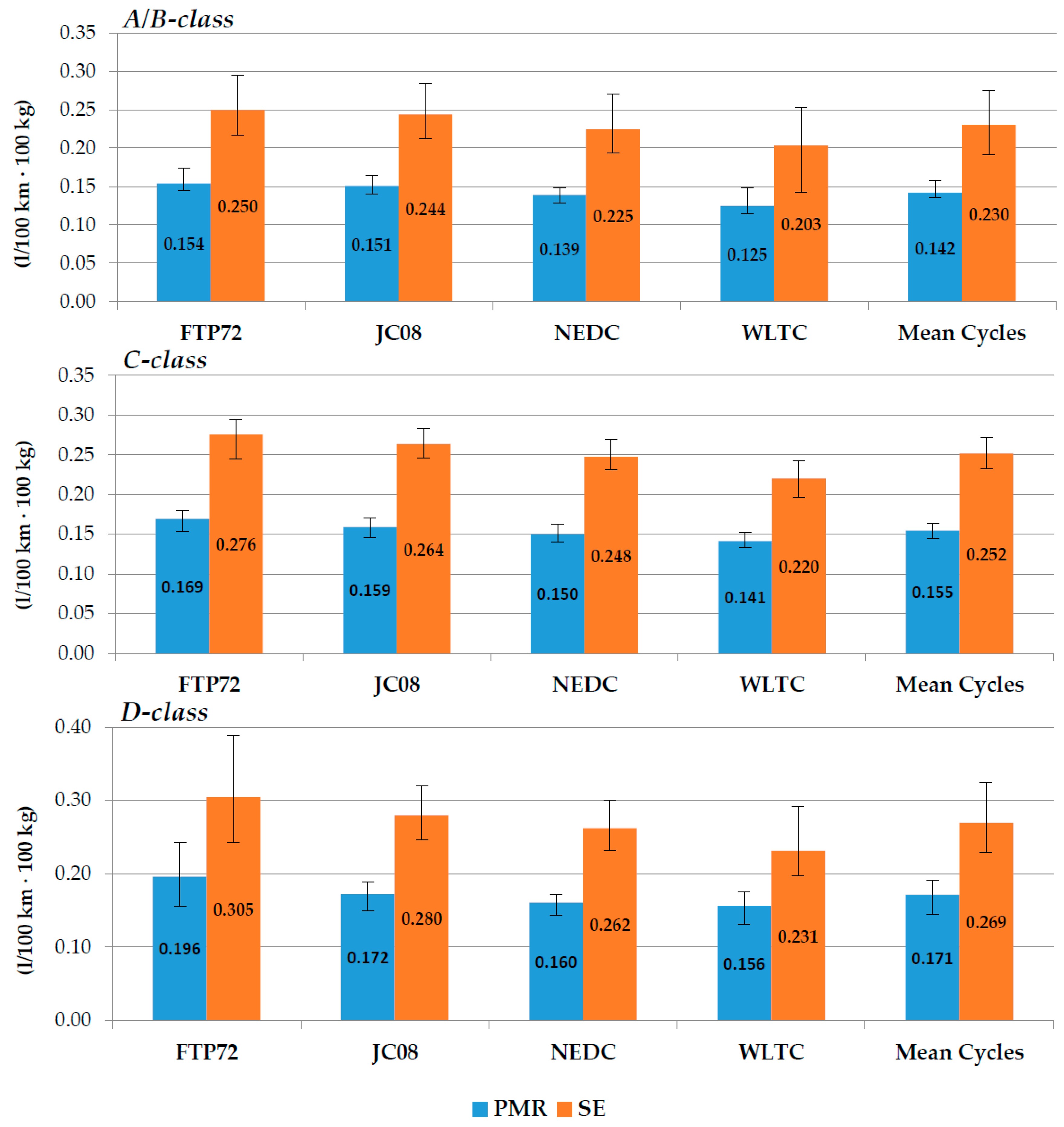
- PMR: FRVFTP72_PMR, FRVJC08_PMR, FRVNEDC_PMR, FRVWLTC_PMR, and FRVMeanCycles_PMR; and
- -
- SE: FRVFTP72_SE, FRVJC08_SE, FRVNEDC_SE, FRVWLTC_SE, FRVMeanCycles_SE.
- -
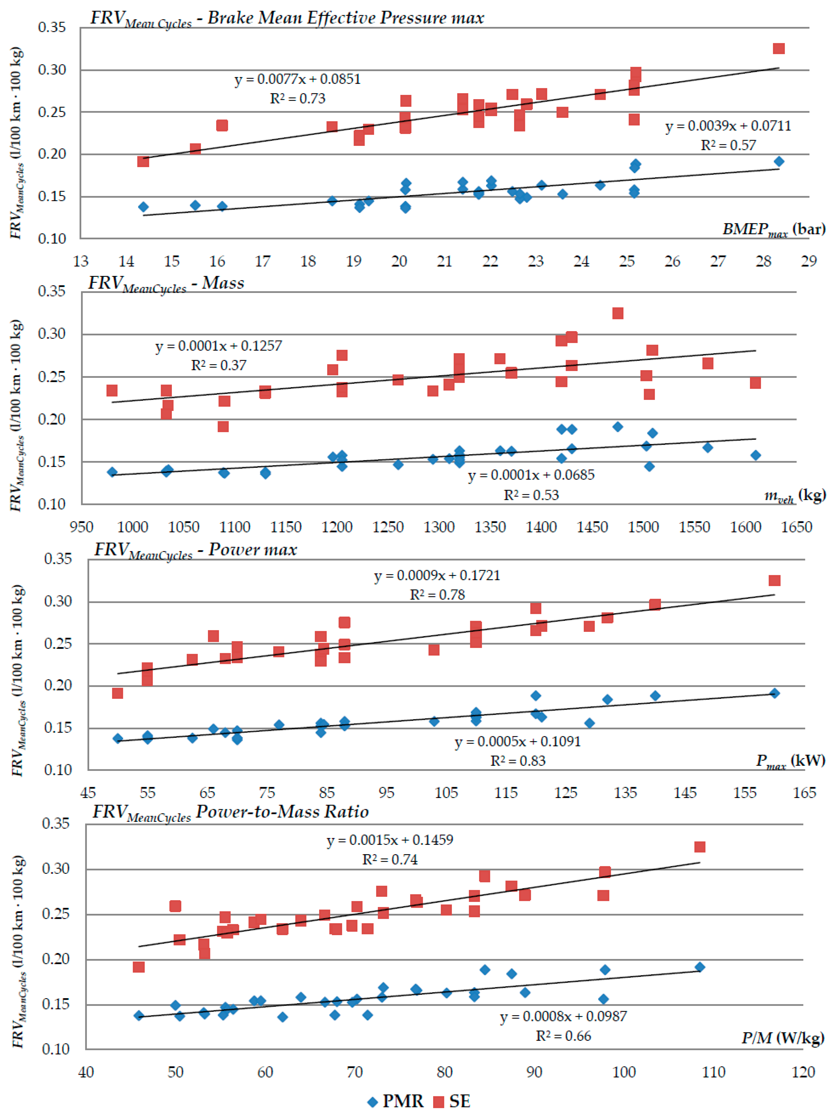
- The highest correlation is for Pmax. R2 is about 0.8 for all cycles (except FRVWLTC_SE for which it is 0.55) with a value of 0.83 and 0.78, respectively, for FRVMeanCycles_PMR and FRVMeanCycles_SE;
- -
- The lowest correlation is for mveh (R2 ranges between a minimum of 0.21 for FRVWLTC_SE and a maximum of 0.59 for FRVWLTC_PMR);
- -
- Intermediate values of R2 refer to PMR and BMEP.
3.2. Environmental Modelling
- -
- PMR: the FRV is obtained from the regression line of FRVMeanCycles_PMR in function of Pmax through the maximum power of the generic application (see Figure 3);
- -
- SE: The FRV is obtained from the regression line of FRVMeanCycles_SE in function of Pmax through the maximum power of the generic application (see Figure 3).
- -
- The amount of FC saved during operation (FCuse_sav) has a leading role in the economy of the overall plan. On the one hand, FCuse_sav fixes the amount of fuel whose avoided production is assessed by WTT process. On the other hand, FCuse_sav determines the amount of TTW air emissions saved during operation (see Equations (7)–(15));
- -
- FCuse_sav scales linearly with the saved mass on the basis of the FRV coefficient;
- -
- The amount of air emissions saved during operation (CO2BIO_use_sav, CO2FOS_use_sav, and SO2use_sav) scales linearly with the amount of FC saved during operation (FCuse_sav);
- -
- Considering the typology of air emissions, only CO2 and SO2 are taken into account. Such a choice appears to be reasonable because FC saving involved by mass reduction only influences CO2 and SO2 emissions while it has no effect on the so-called “limited emissions” (i.e., NOx, HC, etc.). Indeed, CO2 and SO2 emissions scale linearly with the amount of FC basing on fuel C and S content while the limited emissions depend exclusively on the number of travelled kilometres as they are treated by exhaust gas treatment system.
3.3. Application to Real Case Study
4. Conclusions
Author Contributions
Conflicts of Interest
References
- Hawkins, T.R.; Singh, B.; Majeau-Bettez, G.; Stromman, A.H. Comparative environmental life cycle assessment of conventional and electric vehicles. J. Ind. Ecol. 2012, 17, 53e64. [Google Scholar] [CrossRef]
- Witik, R.A.; Payet, J.; Michaud, V.; Ludwig, C.; Manson, J.A.E. Assessing the life cycle costs and environmental performance of lightweight materials in automobile applications. Compos. Part A 2011, 42, 1694–1709. [Google Scholar] [CrossRef]
- Solomon, S.D.; Qin, M.; Manning, Z.; Chen, M.; Marquis, K.B.; Averyt, M.T.; Miller, H.L. (Eds.) Climate Change 2007: The Physical Science Basis—Contribution of Working Group I to the Fourth Assessment Report of the Intergovernmental Panel on Climate Change; Cambridge University Press: Cambridge, UK; New York, NY, USA, 2007.
- The Core Writing Team; Pachauri, R.K.; Reisinger, A. (Eds.) Climate Change 2007: The Synthesis Report—Contribution of Working Groups I, II and III to the Fourth Assessment Report of the Intergovernmental Panel on Climate Change; Intergovernmental Panel on Climate Change: Geneva, Switzerland, 2007.
- World Business Council for Sustainable Development (WBCSD). Mobility 2030: Meeting the Challenges to Sustainability—The Sustainable Mobility Project. Available online: https://www.oecd.org/sd-roundtable/papersandpublications/39360485.pdf (accessed on 24 March 2016).
- Berzi, L.; Delogu, M.; Pierini, M. A comparison of Electric Vehicles use-case scenarios—Application of a simulation framework to vehicle design optimization and energy consumption assessment. In Proceedings of the 17th IEEE International Conference on Environment and Electrical Engineering, Florence, Italy, 7–10 June 2016.
- Dattilo, C.A.; Delogu, M.; Berzi, L.; Pierini, M. A sustainability analysis for Electric Vehicles Batteries including aging phenomena. In Proceedings of the 17th IEEE International Conference on Environment and Electrical Engineering, Florence, Italy, 7–10 June 2016.
- Moawad, A.; Sharer, P.; Rousseau, A. Light-Duty Vehicle Fuel Consumption Displacement Potential up to 2045; ANL/ESD/11-4; Argonne National Laboratory: Lemont, IL, USA, 2013.
- O’Neill, B.C.; Oppenheimer, M. Climate change: Dangerous climate impacts and the Kyoto Protocol. Science 2002, 296, 1971–1972. [Google Scholar] [CrossRef] [PubMed]
- Steffen, W.; Noble, I.; Canadell, J.; Apps, M.; Schulze, E.-D.; Jarvis, P.G. The terrestrial carbon cycle: Implications for the Kyoto Protocol. Science 1998, 280, 1393–1394. [Google Scholar]
- Schmidt, W.P.; Dahlqvist, E.; Finkbeiner, M.; Krinke, S.; Lazzari, S.; Oschmann, D.; Pichon, S.; Thiel, C. Life cycle assessment of lightweight and end-of-life scenarios for generic compact class veh icles. Int. J. Life Cycle Assess. 2004, 9, 405–416. [Google Scholar] [CrossRef]
- Koffler, C. Automobile Produkt-Ökobilanzierung. Master’s Thesis, Technische Universität Darmstadt, Darmstadt, Germany, 2007. [Google Scholar]
- Koffler, C.; Rodhe-Branderburger, K. On the calculation of fuel savings through lightweight design in automotive life cycle assessments. Int. J. Life Cycle Assess. 2010, 15, 128–135. [Google Scholar] [CrossRef]
- Ribeiro, C.; Ferreira, J.V.; Partidàrio, P. Life Cycle Assessment of a multi-material car component. Int. J. Life Cycle Assess. 2007, 5, 336–345. [Google Scholar] [CrossRef]
- Nemry, F.; Leduc, G.; Mongelli, I.; Uihlein, A. Environmental Improvement of Passenger Cars, (IMPRO-car); Joint Research Center, European Commission: Brussels, Belgium, 2008. [Google Scholar]
- Rodhe-Branderburger, K.; Obernolte, J. CO2-Potential durch Leichtbau in Pkw. Mater. Test. 2008, 51, 55–63. [Google Scholar] [CrossRef]
- Siskos, P.; Capros, P.; De Vita, A. CO2 and energy efficiency car standards in the EU in the context of a decarbonisation strategy: A model-based policy assessment. Energy Policy 2015, 84, 22–34. [Google Scholar] [CrossRef]
- Stichling, J. Life cycle considerations for lightweight automotive design. In Proceedings of the International Conference: Innovative Developments for Lightweight Vehicle Structures, Wolfsburg, Germany, 26−27 May 2009; pp. 209–218.
- Berzi, L.; Delogu, M.; Pierini, M. Development of driving cycles for electric vehicles in the context of the city of Florence. Transp. Res. Part D Transp. Environ. 2016, 47, 299–322. [Google Scholar] [CrossRef]
- Kim, H.C.; Wallington, T.J. Life-cycle energy and greenhouse gas emission benefits of lightweight in automobiles: Review and harmonization. Environ. Sci. Technol. 2013, 47, 6089–6097. [Google Scholar] [CrossRef] [PubMed]
- Kelly, J.C.; Sullivan, J.L.; Burnham, A.; Elgowainy, A. Impacts of Vehicle Weight Reduction via Material Substitution on Life-Cycle Greenhouse Gas Emissions. Environ. Sci. Technol. 2015, 49, 12535–12542. [Google Scholar] [CrossRef] [PubMed]
- Mayyas, A.T.; Qattawi, A.; Mayyas, A.R.; Omar, M. Quantifiable measures of sustainability: A case study of materials selection for eco-lightweight auto-bodies. J. Clean. Prod. 2013, 40, 177–189. [Google Scholar] [CrossRef]
- Raugei, M.; Morrey, D.; Hutchinson, A.; Winfield, P. A coherent life cycle assessment of a range of lightweight strategies for compact vehicles. J. Clean. Prod. 2015, 108, 1168–1176. [Google Scholar] [CrossRef]
- Berzi, L.; Delogu, M.; Giorgetti, A.; Pierini, M. On-field investigation and process modelling of End-of-Life Vehicles treatment in the context of Italian craft-type Authorized Treatment Facilities. Waste Manag. 2013, 33, 892–906. [Google Scholar] [CrossRef] [PubMed]
- Berzi, L.; Delogu, M.; Pierini, M.; Romoli, F. Evaluation of the end-of-life performance of a hybrid scooter with the application of recyclability and recoverability assessment methods. Resour. Conserv. Recycl. 2016, 108, 140–155. [Google Scholar] [CrossRef]
- Ciacci, L.; Marselli, L.; Passarini, F.; Santini, A.; Vassura, I. A comparison among different automotive shredder residue treatment processes. Int. J. Life Cycle Assess. 2010, 15, 896–906. [Google Scholar] [CrossRef]
- Das, S. The Life-Cycle Impacts of Aluminium Body-in-White Automotive Material. J. Miner. Met. Mater. Soc. 2000, 52, 41–44. [Google Scholar] [CrossRef]
- Funazaki, A.; Taneda, K.; Tahara, K.; Inaba, A. Automobile life cycle assessment issues at end-of-life and recycling. JSAE Rev. 2003, 24, 381–386. [Google Scholar] [CrossRef]
- Delogu, M.; Zanchi, L.; Maltese, S.; Bonoli, A.; Pierini, M. Environmental and Economic Life Cycle Assessment of a lightweight solution for an automotive component: A comparison between talc-filled and hollow glass microspheres-reinforced polymer composites. J. Clean. Prod. 2016, 139, 548–560. [Google Scholar] [CrossRef]
- Geyer, R. Parametric Assessment of Climate Change Impacts of Automotive Material Substitution. Environ. Sci. Technol. 2008, 18, 6973–6979. [Google Scholar] [CrossRef]
- Grujicic, M.; Sellappan, V.; He, T.; Seyr, N.; Obieglo, A.; Erdmann, M.; Holzleitner, J. Total Life Cycle-Based Materials Selection for Polymer Metal Hybrid Body-in-White Automotive Components. J. Mater. Eng. Perform. 2009, 18, 111–128. [Google Scholar] [CrossRef]
- Kim, K.H.; Joung, H.T.; Nam, H.; Seo, Y.C.; Hong, J.H.; Yoo, T.W.; Lim, B.S.; Park, J.H. Management status of end-of-life vehicles and characteristics of automobile shredder residues in Korea. Waste Manag. 2004, 24, 533–540. [Google Scholar] [CrossRef] [PubMed]
- Rajendran, S.; Scelsi, L.; Hodzic, A.; Soutis, C.; Al-Maadeed, M.A. Environmental impact assessment of composites containing recycled plastics. Resour. Conserv. Recycl. 2012, 60, 131–139. [Google Scholar] [CrossRef]
- Zanchi, L.; Delogu, M.; Ierides, M.; Vasiliadis, H. Life cycle assessment and life cycle costing as supporting tools for EVs lightweight design. Smart Innov. Syst. Technol. 2016, 52, 335–348. [Google Scholar]
- Del Pero, F.; Delogu, M.; Pierini, M.; Bonaffini, D. Life Cycle Assessment of a heavy metro train. J. Clean. Prod. 2015, 87, 787–799. [Google Scholar] [CrossRef]
- Finkbeiner, M.; Hoffmann, R. Application of Life Cycle Assessment for the Environmental Certificate of the Mercedes-Benz S-Class (7 pp). Int. J. Life Cycle Assess. 2006, 11, 240–246. [Google Scholar] [CrossRef]
- Koffler, C. Life cycle assessment of automotive lightweight through polymers under US boundary conditions. Int. J. Life Cycle Assess. 2013, 19, 538–545. [Google Scholar] [CrossRef]
- Delogu, M.; Del Pero, F.; Romoli, F.; Pierini, M. Life cycle assessment of a plastic air intake manifold. Int. J. Life Cycle Assess. 2015, 20, 1429–1443. [Google Scholar] [CrossRef]
- Delogu, M.; Del Pero, F.; Berzi, L.; Pierini, M.; Bonaffini, D. End-of-Life in the Railway Sector: Analysis of Recyclability and Recoverability for Different Vehicle Case Studies. Available online: http://www.sciencedirect.com/science/article/pii/S0956053X16305396 (accessed on 10 April 2016).
- Spielmann, M.; Althaus, H.J. Can a prolonged use of a passenger car reduce environmental burdens? Life Cycle analysis of Swiss passenger cars. J. Clean. Prod. 2006, 15, 1122–1134. [Google Scholar]
- Alves, C.; Ferrao, P.M.C.; Silva, A.J.; Reis, L.G.; Freitas, M.; Rodrigues, L.B. Ecodesign of automotive components making use of jute fiber composites. J. Clean. Prod. 2010, 18, 313–327. [Google Scholar] [CrossRef]
- Du, J.D.; Han, W.J.; Peng, Y.H.; Gu, C.C. Potential for reducing GHG emissions and energy consumption from implementing the aluminum intensive vehicle fleet in China. Energy 2010, 35, 4671–4678. [Google Scholar]
- Duflou, J.R.; De Moor, J.; Verpoest, I.; Dewulf, W. Environmental impact analysis of composite use in car manufacturing. CIRP Ann. Manuf. Technol. 2009, 58, 9–12. [Google Scholar] [CrossRef]
- Luz, S.; Pires, A.C.; Ferrao, P.M. Environmental benefits of substituting talc by sugarcane bagasse fibres as reinforcement in polypropylene composites: Eco-design and LCA strategy for automotive components. Resour. Conserv. Recyc. 2010, 54, 1135–1144. [Google Scholar] [CrossRef]
- Zah, R.; Hischier, R.; Leao, A.L.; Braun, I. Curauà fibers in the automobile industry—A sustainability assessment. J. Clean. Prod. 2006, 15, 1032–1040. [Google Scholar] [CrossRef]
- Ridge, L. EUCAR—Automotive LCA guidelines—phase 2, Total Life Cycle Conference and Exposition; SAE Technical Paper 982185; Society of Automotive Engineers (SAE): Graz, Austria, 1997. [Google Scholar]
- Ribeiro, I.; Peças, P.; Silva, A.; Henriques, E. Life Cycle Engineering Methodology Applied to Material Selection, a Fender Case Study. J. Clean. Prod. 2008, 16, 1887–1899. [Google Scholar] [CrossRef]
- Subic, A.; Schiavone, F. Design-oriented application of LCA to an automotive system. In Proceedings of the 5th Australian Conference on Life Cycle Assessment, Achieving Benefits from Managing Life Cycle impacts, Melbourne, Austrlia, 22−24 November 2006.
- Del Pero, F.; Delogu, M.; Pierini, M. Assessing the effect of lightweighting in automotive LCA perspective: Estimation of mass-induced fuel consumption reduction for gasoline turbocharged vehicles. J. Clean. Prod. 2016. submitted. [Google Scholar]
- Eberle, R.; Franze, H.A. Modelling the Use Phase of Passenger Cars in LCI; SAE Technical Paper 982179; Society of Automotive Engineers (SAE): Graz, Austria, 1998. [Google Scholar]
- Kim, H.C.; Wallington, T.J. Life Cycle Assessment of Vehicle Lightweighting: A Physics-Based Model of Mass-Induced Fuel Consumption. Environ. Sci. Technol. 2013, 47, 14358–14366. [Google Scholar] [CrossRef] [PubMed]
- Kim, H.C.; Wallington, T.J.; Sullivan, J.L.; Keoleian, G.A. Life Cycle Assessment of Vehicle Lightweighting: Novel Mathematical Methods to Estimate Use-Phase Fuel Consumption. Environ. Sci. Technol. 2015, 49, 10209–10216. [Google Scholar] [CrossRef] [PubMed]
- Pagerit, S.; Sharer, P.; Rousseau, A. Fuel Economy Sensitivity to Vehicle Mass for Advanced Vehicle Powertrains; SAE Paper No. 2006-01-0665; SAE International: Detroit, MI, USA, 2006. [Google Scholar]
- Wohlecker, R.; Johannaber, M.; Espig, M. Determination of Weight Elasticity of Fuel Economy for ICE, Hybrid and Fuel Cell Vehicles; SAE Paper No. 2007-01-0343; SAE International: Detroit, MI, USA, 2007. [Google Scholar]
- Casadei, A.; Broda, R. Impact of Vehicle Weight Reduction on Fuel Economy for Various Vehicle Architectures. Available online: http://www.drivealuminum.org/wp-content/uploads/2016/07/Ricardo_Impact-of-Vehicle-Weight-Reduction-on-Fuel-Economy-for-Various-Vehicle-Architectures.pdf (accessed on 7 February 2016).
- Redelbach, M.; Klotzke, M.; Friedrich, H.E. Impact of lightweight design on energy consumption and cost effectiveness of alternative powertrain concepts. In Proceedings of the European Electric Vehicle Conference, Brüssel, Belgien, 19−22 November 2012.
- Marotta, A.; Tutuianu, M. Europe-Centric Light Duty Test Cycle and Differences with Respect to the WLTP Cycle; JRC (Joint Research Centre) Scientific and Policy Reports; European Commission: Varese, Italy, 2012. [Google Scholar]
- Mock, P. Inertia Classes Proposal. WLTP-DTP-LabProcICE-077. Submission to the UNECE GRPE Informal Subgroup on the Development of a Worldwide Harmonized Light Vehicles Test Procedure (WLTP-DTP). Available online: http://www.theicct.org/sites/default/files/publications/WLTP_inertia_workingpaper_2011.pdf (accessed on 2 March 2016).
- Tutuianu, M.; Marotta, A.; Steve, H.; Ericsson, E.; Haniu, T.; Ichikawa, N.; Ishii, H. Development of a World-Wide Worldwide Harmonized Light Duty Driving Test Cycle (WLTC). Available online: https://www.unece.org/fileadmin/DAM/trans/doc/2013/wp29grpe/GRPE-67-03.pdf (accessed on 24 March 2016).
- United States Environmental Protection Agency (EPA) Home Page. Available online: http://www3.epa.gov/ (accessed on 18 January 2015).
- United Nations Economic Commission for Europe (UNECE) Home Page. Available online: http://www.unece.org/trans/welcome.html (accessed on 4 March 2015).
- Barlow, T.J.; Latham, S.; McCrae, I.S.; Boulter, P.G. A Reference Book of Driving Cycles for Use in the Measurement of Road Vehicle Emissions; TRL Published Project Report; TRL (Transport Research Laboratory): Berkshire, UK, 2009. [Google Scholar]
- Kuhlwein, J.; German, J.; Baudiradekar, A. Development of Test Cycle Conversion among Worldwide Light-Duty Vehicle CO2 Emission Standard. Available online: http://www.theicct.org/sites/default/files/publications/ICCT_LDV-test-cycle-conversion-factors_sept2014.pdf (accessed on 3 April 2016).


| Reference Mass-Configuration—Variable Model Parameters—Reference Car Models | |||||
|---|---|---|---|---|---|
| A/B-Class | C-Class | D-Class | |||
| Case Study | Vehicle Model | Case Study | Vehicle Model | Case Study | Vehicle Model |
| 1 | A. R. MiTo 1.6 JTDm 120cv | 11 | A. R. Giulietta 1.6 JTDm 105cv | 23 | BMW 318d 2.0 150cv |
| 2 | CITROEN C3 1.4 HDi 70cv | 12 | A. R. Giulietta 2.0 JTDm 150cv | 24 | BMW 320d 2.0 163cv |
| 3 | CITROEN C3 1.6 HDi 115cv | 13 | A. R. Giulietta 2.0 JTDm 175cv | 25 | BMW 320d 2.0 190cv |
| 4 | FIAT Cinquecento 1.3 MJT 95cv | 14 | CITROEN C4 1.6 HDi 90cv | 26 | BMW 325d 2.0 218cv |
| 5 | FIAT Panda 1.3 MJT 75cv | 15 | CITROEN C4 1.6 HDi 115cv | 27 | CITROEN C5 1.6 HDi 115cv |
| 6 | FIAT Punto 1.3 MJT 75cv | 16 | CITROEN C4 2.0 HDi 150cv | 28 | CITROEN C5 2.0 HDi 140cv |
| 7 | FIAT Punto 1.3 MJT 85cv | 17 | FIAT Bravo 1.6 MJT 90cv | 29 | CITROEN C5 2.0 HDi 165cv |
| 8 | FIAT Punto 1.3 MJT 95cv | 18 | FIAT Bravo 1.6 MJT 120cv | 30 | FORD Mondeo 1.6 TDCi 115cv |
| 9 | FORD Fiesta 1.5 TDCi 75cv | 19 | FIAT Bravo 1.6 MJT 165cv | 31 | FORD Mondeo 2.0 TDCi 150cv |
| 10 | FORD Fiesta 1.6 TDCi 95cv | 20 | FORD Focus 1.5 TDCi 95 cv | 32 | FORD Mondeo 2.0 TDCi 180cv |
| 21 | FORD Focus 1.5 TDCi 120cv | ||||
| 22 | FORD Focus 2.0 TDCi 150cv | ||||
| TTW Process | ||
|---|---|---|
| Parameters | GaBi6 Flows | |
| INPUT | Amount of Fuel Consumption saved during operation thanks to light-weighting (FCuse_sav) | Diesel—Refinery products (kg) |
| OUTPUT | Amount of biogenic CO2 emission saved during operation thanks to light-weighting (CO2BIO_use_sav) | Carbon dioxide (biotic)—Inorganic emissions to air (g) |
| Amount of fossil CO2 emission saved during operation thanks to light-weighting (CO2FOS_use_sav) | Carbon dioxide (fossil)—Inorganic emissions to air (g) | |
| Amount of SO2 emission saved during operation thanks to light-weighting (SO2_use_sav) | Sulphur dioxide—Inorganic emissions to air (kg) | |
| TTW Equations | |||
|---|---|---|---|
| INPUT | (6) | ||
| OUTPUT | (7) | ||
| Where: | (8) | ||
| (9) | |||
| (10) | |||
| (11) | |||
| Where: | (12) | ||
| (13) | |||
| Where: | (14) | ||
| (15) | |||
| Legend: FRV = Fuel Reduction Value (l/100 km × 100kg); masssav = saved mass thanks to lightweighting (kg); mileageuse = total mileage during operation (km); ρfuel = fuel density (kg/l); CO2BIO_veh_km = per-kilometre biogenic CO2 emission of reference vehicle (g/km); FCuse_veh = amount of Fuel Consumption during operation of reference vehicle (g/km); CO2_veh_km = per-kilometre CO2 emission of reference vehicle (g/km); share CO2BIO = share of biogenic C in fuel; sharemw shareru shareur = share of total mileage respectively for motorway, rural and urban route; CO2_veh_km_mw, CO2_veh_km_ru, CO2_veh_km_ur = per-kilometre CO2 emission of reference vehicle respectively for motorway, rural and urban route (g/km); FCveh_100km = per-100 kilometre Fuel Consumption of reference vehicle (l/100 km); CO2FOS_veh_km = per-kilometre fossil CO2 emission of reference vehicle (g/km); SO2_veh_km = per-kilometre SO2 emission of reference vehicle (kg/km); ppmsuphur = sulphur content in fuel (ppm); | |||
| FRV (L/100 km × 100 kg) | |||||||||||
|---|---|---|---|---|---|---|---|---|---|---|---|
| PMR | SE | ||||||||||
| Vehicle Class | Case Study | FTP72 (FRVFTP72_PMR) | JC08 (FRVJC08_PMR) | NEDC (FRVNEDC_PMR) | WLTC (FRVWLTC_PMR) | Mean Cycles (FRVMeanCycles_PMR) | FTP72 (FRVFTP72_SE) | JC08 (FRVJC08_SE) | NEDC (FRVNEDC_SE) | WLTC (FRVWLTC_SE) | Mean Cycles (FRVMeanCycles_SE) |
| A/B | 1 | 0.173 | 0.165 | 0.148 | 0.146 | 0.158 | 0.295 | 0.284 | 0.270 | 0.253 | 0.276 |
| 2 | 0.153 | 0.140 | 0.143 | 0.115 | 0.138 | 0.217 | 0.212 | 0.194 | 0.142 | 0.191 | |
| 3 | 0.174 | 0.157 | 0.145 | 0.148 | 0.156 | 0.281 | 0.275 | 0.259 | 0.220 | 0.259 | |
| 4 | 0.149 | 0.150 | 0.137 | 0.117 | 0.138 | 0.253 | 0.245 | 0.224 | 0.214 | 0.234 | |
| 5 | 0.145 | 0.151 | 0.146 | 0.122 | 0.141 | 0.239 | 0.237 | 0.218 | 0.173 | 0.217 | |
| 6 | 0.147 | 0.149 | 0.136 | 0.116 | 0.137 | 0.235 | 0.235 | 0.215 | 0.202 | 0.222 | |
| 7 | 0.150 | 0.153 | 0.130 | 0.120 | 0.138 | 0.246 | 0.240 | 0.213 | 0.225 | 0.231 | |
| 8 | 0.150 | 0.148 | 0.129 | 0.117 | 0.136 | 0.250 | 0.241 | 0.221 | 0.223 | 0.234 | |
| 9 | 0.149 | 0.143 | 0.137 | 0.129 | 0.140 | 0.227 | 0.226 | 0.207 | 0.166 | 0.207 | |
| 10 | 0.149 | 0.150 | 0.137 | 0.117 | 0.138 | 0.253 | 0.245 | 0.224 | 0.214 | 0.234 | |
| C | 11 | 0.168 | 0.159 | 0.148 | 0.141 | 0.154 | 0.262 | 0.253 | 0.235 | 0.214 | 0.241 |
| 12 | 0.180 | 0.167 | 0.154 | 0.152 | 0.163 | 0.294 | 0.282 | 0.266 | 0.240 | 0.271 | |
| 13 | 0.171 | 0.161 | 0.149 | 0.143 | 0.156 | 0.291 | 0.280 | 0.270 | 0.243 | 0.271 | |
| 14 | 0.154 | 0.146 | 0.142 | 0.137 | 0.145 | 0.245 | 0.247 | 0.233 | 0.206 | 0.233 | |
| 15 | 0.166 | 0.157 | 0.149 | 0.138 | 0.153 | 0.261 | 0.252 | 0.231 | 0.206 | 0.238 | |
| 16 | 0.174 | 0.160 | 0.156 | 0.144 | 0.159 | 0.281 | 0.266 | 0.252 | 0.214 | 0.253 | |
| 17 | 0.165 | 0.153 | 0.140 | 0.138 | 0.149 | 0.289 | 0.269 | 0.246 | 0.233 | 0.259 | |
| 18 | 0.167 | 0.159 | 0.149 | 0.136 | 0.153 | 0.273 | 0.259 | 0.245 | 0.220 | 0.249 | |
| 19 | 0.179 | 0.170 | 0.154 | 0.150 | 0.163 | 0.294 | 0.283 | 0.269 | 0.239 | 0.271 | |
| 20 | 0.160 | 0.154 | 0.141 | 0.133 | 0.147 | 0.273 | 0.258 | 0.240 | 0.216 | 0.247 | |
| 21 | 0.166 | 0.157 | 0.153 | 0.137 | 0.153 | 0.259 | 0.246 | 0.234 | 0.196 | 0.234 | |
| 22 | 0.179 | 0.162 | 0.163 | 0.147 | 0.163 | 0.286 | 0.268 | 0.249 | 0.216 | 0.255 | |
| D | 23 | 0.187 | 0.168 | 0.158 | 0.150 | 0.166 | 0.297 | 0.273 | 0.259 | 0.224 | 0.263 |
| 24 | 0.220 | 0.189 | 0.170 | 0.175 | 0.189 | 0.340 | 0.298 | 0.278 | 0.253 | 0.292 | |
| 25 | 0.226 | 0.188 | 0.172 | 0.168 | 0.189 | 0.346 | 0.305 | 0.287 | 0.249 | 0.297 | |
| 26 | 0.243 | 0.182 | 0.168 | 0.173 | 0.192 | 0.388 | 0.320 | 0.300 | 0.292 | 0.325 | |
| 27 | 0.156 | 0.149 | 0.143 | 0.131 | 0.145 | 0.243 | 0.246 | 0.232 | 0.197 | 0.230 | |
| 28 | 0.169 | 0.161 | 0.153 | 0.149 | 0.158 | 0.257 | 0.259 | 0.244 | 0.212 | 0.243 | |
| 29 | 0.184 | 0.170 | 0.158 | 0.156 | 0.167 | 0.294 | 0.277 | 0.261 | 0.232 | 0.266 | |
| 30 | 0.166 | 0.159 | 0.151 | 0.141 | 0.154 | 0.266 | 0.260 | 0.244 | 0.207 | 0.244 | |
| 31 | 0.197 | 0.170 | 0.160 | 0.148 | 0.169 | 0.291 | 0.264 | 0.243 | 0.208 | 0.252 | |
| 32 | 0.212 | 0.184 | 0.171 | 0.169 | 0.184 | 0.323 | 0.294 | 0.271 | 0.237 | 0.281 | |
| Coefficient of Determination R2 | ||||||||||
|---|---|---|---|---|---|---|---|---|---|---|
| FRVFTP72 | FRVJC08 | FRVNEDC | FRVWLTC | FRVMeanCycles | ||||||
| PMR | SE | PMR | SE | PMR | SE | PMR | SE | PMR | SE | |
| Maximum Brake Mean Effective Pressure (BMEPmax) | 0.55 | 0.68 | 0.61 | 0.71 | 0.40 | 0.69 | 0.57 | 0.67 | 0.57 | 0.73 |
| Vehicle mass (mveh) | 0.45 | 0.36 | 0.46 | 0.41 | 0.53 | 0.43 | 0.59 | 0.21 | 0.53 | 0.37 |
| Maximum Power (Pmax) | 0.79 | 0.78 | 0.78 | 0.80 | 0.74 | 0.82 | 0.78 | 0.55 | 0.83 | 0.78 |
| Power-to-Mass Ratio (PMR) | 0.65 | 0.72 | 0.66 | 0.73 | 0.56 | 0.75 | 0.58 | 0.57 | 0.66 | 0.74 |
| FRV (L/100 km·100 kg) | |
|---|---|
| PMR | SE |
| FIAT Panda 1.3. MJT (Model Year 2016) | |
|---|---|
| Curb mass (kg) | 1045 |
| Propulsion | Diesel Turbocharged |
| Engine displacement (cc) | 1248 |
| Maximum power (kW) | 70 |
| Emission stage | EURO 6 |
| Mixed consumption (L/100 km) | 3.6 |
| CO2 emissions (g/km) | 94 |
| SO2 emissions (g/km) | 6.42 × 10⁻⁴ |
| Use stage (km) | 150,000 |
© 2016 by the authors; licensee MDPI, Basel, Switzerland. This article is an open access article distributed under the terms and conditions of the Creative Commons Attribution (CC-BY) license (http://creativecommons.org/licenses/by/4.0/).
Share and Cite
Delogu, M.; Del Pero, F.; Pierini, M. Lightweight Design Solutions in the Automotive Field: Environmental Modelling Based on Fuel Reduction Value Applied to Diesel Turbocharged Vehicles. Sustainability 2016, 8, 1167. https://doi.org/10.3390/su8111167
Delogu M, Del Pero F, Pierini M. Lightweight Design Solutions in the Automotive Field: Environmental Modelling Based on Fuel Reduction Value Applied to Diesel Turbocharged Vehicles. Sustainability. 2016; 8(11):1167. https://doi.org/10.3390/su8111167
Chicago/Turabian StyleDelogu, Massimo, Francesco Del Pero, and Marco Pierini. 2016. "Lightweight Design Solutions in the Automotive Field: Environmental Modelling Based on Fuel Reduction Value Applied to Diesel Turbocharged Vehicles" Sustainability 8, no. 11: 1167. https://doi.org/10.3390/su8111167
APA StyleDelogu, M., Del Pero, F., & Pierini, M. (2016). Lightweight Design Solutions in the Automotive Field: Environmental Modelling Based on Fuel Reduction Value Applied to Diesel Turbocharged Vehicles. Sustainability, 8(11), 1167. https://doi.org/10.3390/su8111167