
Spatial Preference Heterogeneity for Integrated River Basin Management: The Case of the Shiyang River Basin, China


Abstract
:1. Introduction
2. Study Area and the Sample
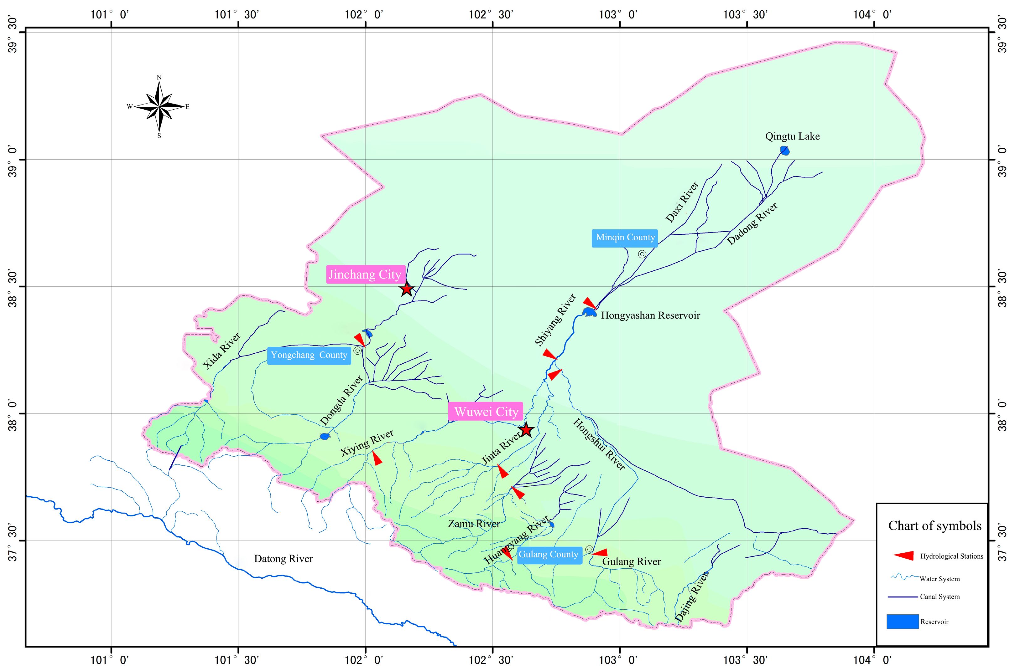
2.1. The Shiyang River Basin
2.2. The Sample
3. Methodology
3.1. Choice Experiment
3.2. Econometric Analysis
4. Result and Discussion
4.1. Data Screening for Inconsistent Responses
4.2. Spatial Preference Heterogeneity
4.3. The Willingness to Pay Estimate
5. Conclusions
Acknowledgement
Author Contributions
Conflicts of Interest
Appendix A

| Variables | Sex (Male = 1) | Age | Gross Income (¥1000) | Education (Below High School = 1) | Job (Farmer = 1) | Family Size | Dependent Child or Elder (Yes = 1) | Cadre (Yes = 1) | |
|---|---|---|---|---|---|---|---|---|---|
| USB | Min | 0 | 15 | 2.39 | 0 | 0 | 1 | 0 | 0 |
| max | 1 | 78 | 156 | 1 | 1 | 9 | 1 | 1 | |
| mean | 0.6 | 40.6 | 42.5 | 0.47 | 0.44 | 4.0 | 0.85 | 0.26 | |
| St.dev | 0.48 | 14.11 | 26.5 | 0.49 | 0.49 | 1.58 | 0.36 | 0.44 | |
| MSB | min | 0 | 14 | 1.1 | 0 | 0 | 1 | 0 | 0 |
| max | 1 | 81 | 159.2 | 1 | 1 | 8 | 1 | 1 | |
| mean | 0.64 | 40.7 | 46.84 | 0.46 | 0.47 | 3.86 | 0.85 | 0.29 | |
| St.dev | 0.48 | 11.78 | 27.68 | 0.49 | 0.49 | 1.26 | 0.36 | 0.45 | |
| LSB | min | 0 | 20 | 1.5 | 0 | 0 | 1 | 0 | 0 |
| max | 1 | 75 | 150 | 1 | 1 | 8 | 1 | 1 | |
| mean | 0.7 | 44.0 | 47.2 | 0.42 | 0.59 | 3.9 | 0.87 | 0.21 | |
| St.dev | 0.46 | 9.8 | 28.8 | 0.49 | 0.49 | 1.16 | 0.34 | 0.42 | |
| pooled data (PD) | min | 0 | 24 | 1.1 | 0 | 0 | 1 | 0 | 0 |
| max | 1 | 81 | 159.2 | 1 | 1 | 9 | 1 | 1 | |
| mean | 0.65 | 41.7 | 46.12 | 0.452 | 0.56 | 3.94 | 0.85 | 0.26 | |
| St.dev | 0.48 | 11.86 | 27.84 | 0.49 | 0.49 | 1.3 | 0.35 | 0.33 |
References
- GWP. Integrated Water Resources Management, 4th ed; Global Water Partnership: Stockholm, Sweden, 2000; p. 71. [Google Scholar]
- Rahaman, M.M.; Varis, O. Integrated water resources management: Evolution, prospects and future challenges. Sustain. Sci. Pract. Policy 2005, 1, 15–21. [Google Scholar]
- Boekhorst, D.G.J.T.; Smits, T.J.M.; Yu, X.B.; Li, L.F.; Lei, G.; Zhang, C. Implementing Integrated River Basin Management in China. Ecol. Soc. 2010, 15, 23. [Google Scholar]
- Song, X.; Ravesteijn, W.; Frostell, B.; Wennersten, R. Managing water resources for sustainable development: The case of integrated river basin management in China. Water Sci. Technol. 2010, 61, 499–506. [Google Scholar] [CrossRef] [PubMed]
- McNally, R.; Tognetti, S. Tackling Poverty and Promoting Sustainable Development: Key Lessons for Integrated River Basin Management; WWF: Godalming, UK, 2002; p. 35. [Google Scholar]
- Harsha, J. IWRM and IRBM concepts envisioned in Indian water policies. Curr. Sci. 2012, 102, 986–990. [Google Scholar]
- Evers, M. An analysis of the requirements for DSS on integrated river basin management. Manag. Environ. Qual. Int. J. 2008, 19, 37–53. [Google Scholar] [CrossRef]
- Molle, F. River-basin planning and management: The social life of a concept. Geoforum 2009, 40, 484–494. [Google Scholar] [CrossRef]
- Yu, H.; Edmunds, M.; Lora-Wainwright, A.; Thomas, D. From principles to localized implementation: Villagers’ experiences of IWRM in the Shiyang River basin, Northwest China. Int. J. Water Resour. D 2014, 30, 588–604. [Google Scholar] [CrossRef]
- Carson, R.T.; Mitchell, R.C. The value of clean water: The public’s willingness to pay for boatable, fishable, and swimmable quality water. Water Resour. Res. 1993, 29, 2445–2454. [Google Scholar] [CrossRef]
- Del Saz-Salazar, S.; Hernández-Sancho, F.; Sala-Garrido, R. The social benefits of restoring water quality in the context of the Water Framework Directive: A comparison of willingness to pay and willingness to accept. Sci. Total Environ. 2009, 407, 4574–4583. [Google Scholar] [CrossRef] [PubMed]
- Glenk, K.; Lago, M.; Moran, D. Public preferences for water quality improvements: Implications for the implementation of the EC Water Framework Directive in Scotland. Water Policy 2011, 13, 645–662. [Google Scholar] [CrossRef]
- Hanley, N.; Wright, R.E.; Alvarez-Farizo, B. Estimating the economic value of improvements in river ecology using choice experiments: An application to the water framework directive. J. Environ. Manag. 2006, 78, 183–193. [Google Scholar] [CrossRef] [PubMed]
- Ramajo-Hernández, J.; del Saz-Salazar, S. Estimating the non-market benefits of water quality improvement for a case study in Spain: A contingent valuation approach. Environ. Sci. Policy 2012, 22, 47–59. [Google Scholar] [CrossRef]
- Perni, Á.; Martínez-Paz, J.; Martínez-Carrasco, F. Social preferences and economic valuation for water quality and river restoration: The Segura River, Spain. Water Environ. J. 2012, 26, 274–284. [Google Scholar] [CrossRef]
- Brouwer, R.; Martin-Ortega, J.; Berbel, J. Spatial preference heterogeneity: A choice experiment. Land Econ. 2010, 86, 552–568. [Google Scholar] [CrossRef]
- Condon, B.; Hodges, A.; Matta, R. Public preferences and values for rural land preservation in Florida. In Proceedings of the American Agricultural Economics Association Annual Meeting, Portland, OR, USA, 29 July–1 August 2007.
- Martin-Ortega, J.; Brouwer, R.; Ojea, E.; Berbel, J. Benefit transfer and spatial heterogeneity of preferences for water quality improvements. J. Environ. Manag. 2012, 106, 22–29. [Google Scholar] [CrossRef] [PubMed]
- Calderon, M.M.; Camacho, L.D.; Carandang, M.G.; Dizon, J.T.; Rebugio, L.L.; Tolentinob, N.L. Willingness to pay for improved watershed management: Evidence from metro manila, Philippines. For. Sci. Technol. 2006, 2, 42–50. [Google Scholar] [CrossRef]
- Amponin, J.A.R.; Bennagen, M.E.C.; Hess, S.; dela Cruz, J.D.S. Willingness to Pay for Watershed Protection by Domestic Water Users in Tuguegarao City, Philippines; Institution for Enviromental Studies: Amsterdam, The Netherlands, 2007; p. 51. [Google Scholar]
- Cao, S.X.; Chen, L.; Shankman, D.; Wang, C.M.; Wang, X.B.; Zhang, H. Excessive reliance on afforestation in China’s arid and semi-arid regions: Lessons in ecological restoration. Earth Sci. Rev. 2011, 104, 240–245. [Google Scholar] [CrossRef]
- Li, W.H. Degradation and restoration of forest ecosystems in China. For. Ecol. Manag. 2004, 201, 33–41. [Google Scholar]
- Wang, X.M.; Zhang, C.X.; Hasi, E.; Dong, Z.B. Has the Three Norths Forest Shelterbelt Program solved the desertification and dust storm problems in arid and semiarid China? J. Arid Environ. 2010, 74, 13–22. [Google Scholar] [CrossRef]
- te Boekhorst, D.; Smits, T.; Xiubo, Y.; Lifeng, L.; Gang, L.; Chen, Z. Implementing integrated river basin management in China. Ecol. Soc. 2010, 15, 99–119. [Google Scholar]
- Schaafsma, M.; Brouwer, R.; Gilbert, A.; van den Bergh, J.; Wagtendonk, A. Estimation of distance-decay functions to account for substitution and spatial heterogeneity in stated preference research. Land Econ. 2013, 89, 514–537. [Google Scholar] [CrossRef]
- Sutherland, R.J.; Walsh, R.G. Effect of distance on the preservation value of water quality. Land Econ. 1985, 61, 281–291. [Google Scholar] [CrossRef]
- Schaafsma, M.; Brouwer, R.; Rose, J. Directional heterogeneity in WTP models for environmental valuation. Ecol. Econ. 2012, 79, 21–31. [Google Scholar] [CrossRef]
- Abildtrup, J.; Garcia, S.; Olsen, S.B.; Stenger, A. Spatial preference heterogeneity in forest recreation. Ecol. Econ. 2013, 92, 67–77. [Google Scholar] [CrossRef]
- Ma, J.; Ding, Z.; Wei, G.; Zhao, H.; Huang, T. Sources of water pollution and evolution of water quality in the Wuwei basin of Shiyang river, Northwest China. J. Environ. Manag. 2009, 90, 1168–1177. [Google Scholar] [CrossRef] [PubMed]
- Li, F.; Zhu, G.; Guo, C. Shiyang River ecosystem problems and Countermeasures. Agric. Sci. 2013, 4, 7. [Google Scholar] [CrossRef]
- Wang, Z.J.; Zheng, H.; Wang, X.F. A Harmonious Water Rights Allocation Model for Shiyang River Basin, Gansu Province, China. Int. J. Water Resour. D 2009, 25, 355–371. [Google Scholar]
- Xie, H.; Burrell, B.C.; Droslte, R. The Shiyang River: A case of water scarcity. Can. Civ. Eng. 2011. Available online: https://csce.ca/wp-content/uploads/2012/04/2011-Summer-issue-vol-28.3.pdf (accessed on 13 August 2013). [Google Scholar]
- Danfeng, S.; Dawson, R.; Baoguo, L. Agricultural causes of desertification risk in Minqin, China. J. Environ. Manag. 2006, 79, 348–356. [Google Scholar] [CrossRef] [PubMed]
- Wei, Y.; Zheng, H. Enforcing the science and policy interface—Experiences from ACEDP Inland River Basin Project. In Proceedings ot the 14th International River Symposium, Brisbane, Australia, 26–29 September 2011.
- Zhao, M.; Yao, L.; Tao, X. What restoration do the public expect? Quantifying Economic value, preferences heterogeneity and regional decision support. In Proceedings of the 2014 CAER_IFPRI Annual International Conference, Yangling, China, 16–17 October 2014; China Agricultural University Press: Yangling, China, 2014; p. 619. [Google Scholar]
- Tang, Z.; Nan, Z.; Liu, J. The Willingness to Pay for Irrigation Water: A Case Study in Northwest China. Glob. Nest J. 2013, 15, 76–84. [Google Scholar]
- Aizaki, H. Package ‘mded’: Measuring the Difference between Two Empirical Distributions. 2015. Available online: https://cran.r-project.org/web/packages/mded/mded.pdf (accessed on 15 June 2015).
- Hanley, N.; Spash, C.L. Cost-Benefit Analysis and the Enviroment; Edward Elgar: Aldershot, UK, 1993; p. 288. [Google Scholar]
- Hensher, D.; Shore, N.; Train, K. Households’ willingness to pay for water service attributes. Environ. Resour. Econ. 2005, 32, 509–531. [Google Scholar] [CrossRef]
- Kosenius, A.K. Heterogeneous preferences for water quality attributes: The Case of eutrophication in the Gulf of Finland, the Baltic Sea. Ecol. Econ. 2010, 69, 528–538. [Google Scholar] [CrossRef]
- Jianjun, J.; Chong, J.; Thuy, T.D.; Lun, L. Public preferences for cultivated land protection in Wenling City, China: A choice experiment study. Land Use Policy 2013, 30, 337–343. [Google Scholar] [CrossRef]
- Hanley, N.; Mourato, S.; Wright, R.E. Choice modelling approaches: A superior alternative for environmental valuation? J. Econ. Surv. 2001, 15, 435–462. [Google Scholar] [CrossRef]
- Carson, R.; Czajkowski, M. The discrete choice experiment approach to environmental contingent valuation. In Handbook of Choice Modelling; Daly, S.H.a.A., Ed.; Edward Elgar Publishing: Cheltenham, UK, 2014. [Google Scholar]
- Sándor, Z.; Wedel, M. Profile construction in experimental choice designs for mixed logit models. Mark. Sci. 2002, 21, 455–475. [Google Scholar] [CrossRef]
- Scarpa, R.; Rose, J.M. Design efficiency for non-market valuation with choice modelling: How to measure it, what to report and why. Aust. J. Agric. Resour. Econ. 2008, 52, 253–282. [Google Scholar] [CrossRef]
- Lancsar, E.; Louviere, J. Conducting discrete choice experiments to inform healthcare decision making. Pharmacoeconomics 2008, 26, 661–677. [Google Scholar] [CrossRef] [PubMed]
- Carson, R.T.; Louviere, J.J.; Wei, E. Alternative Australian climate change plans: The public’s views. Energy Policy 2010, 38, 902–911. [Google Scholar] [CrossRef]
- McFadden, D. Conditional Logit Analysis of Qualitative Choice Behavior. In Frontiers in Economics; Zimmermann, K.F., Ed.; Academic Press: New York, NY, USA, 1973. [Google Scholar]
- Revelt, D.; Train, K. Mixed logit with repeated choices: Households’ choices of appliance efficiency level. Rev. Econ. Stat. 1998, 80, 647–657. [Google Scholar] [CrossRef]
- Lagarde, M. Investigating Attribute Non-Attendance And Its Consequences In Choice Experiments with Latent Class Models. Health Econ. 2013, 22, 554–567. [Google Scholar] [CrossRef] [PubMed]
- Hensher, D.A.; Greene, W.H. The Mixed Logit model: The state of practice. Transportation 2003, 30, 133–176. [Google Scholar] [CrossRef]
- Hensher, D.A.; Rose, J.; Greene, W.H. Applied Choice Analysis: A Primer; Cambridge University Press: Cambridge, UK, 2005; p. 744. [Google Scholar]
- Louviere, J.J.; Hensher, D.A.; Swait, J.D. Stated Choice Methods: Analysis and Applications; Cambridge University Press: Cambridge, UK, 2000. [Google Scholar]
- Kragt, M.E.; Bennett, J.W. Using choice experiments to value catchment and estuary health in Tasmania with individual preference heterogeneity. Aust. J. Agric. Resour. Econ. 2011, 55, 159–179. [Google Scholar] [CrossRef]
- Train, K. Halton Sequences for Mixed Logit. Department of Economics, UCB, 2000. Available online: https://escholarship.org/uc/item/6zs694tp (accessed on 10 December 2013).
- Lusk, J.L.; Schroeder, T.C. Are choice experiments incentive compatible? A test with quality differentiated beef steaks. Am. J. Agric. Econ. 2004, 86, 467–482. [Google Scholar] [CrossRef]
- Hanemann, W.M. Welfare evaluations in contingent valuation information with discrete responses. Am. J. Agric. Econ. 1984, 66, 20. [Google Scholar] [CrossRef]
- Poe, G.L.; Giraud, K.L.; Loomis, J.B. Computational methods for measuring the difference of empirical distributions. Am. J. Agric. Econ. 2005, 87, 353–365. [Google Scholar] [CrossRef]
- Morrison, M.; Bennett, J.; Blamey, R. Valuing improved wetland quality using choice modeling. Water Resour. Res. 1999, 35, 2805–2814. [Google Scholar] [CrossRef]
| Variables | Min | Max | Mean | St.dev | |||
|---|---|---|---|---|---|---|---|
| Sex (male = 1) | 0 | 1 | 0.65 | 0.48 | |||
| Age | 24 | 81 | 41.7 | 11.86 | |||
| Family size | 1 | 9 | 3.94 | 1.3 | |||
| Dependent child or elderly (yes = 1; no = 0) | 0 | 1 | 0.85 | 0.35 | |||
| Have cadre family member (yes = 1; no = 0) | 0 | 1 | 0.26 | 0.33 | |||
| Education Level | % | Head of Household Occupation | % | Household Gross Income (in Yuan per Year) | % | Farm Size (Mean = 14.9 mu) | % |
| Elementary school | 14.91 | farmer | 52.2 | ≤10,000 | 6.65 | Large (40–200 mu) | 7.4 |
| Junior school | 30.28 | officer | 6.54 | 10,000–30,000 | 27.18 | Medium (39–15 mu) | 27.2 |
| High school or college | 20.99 | organ or unit | 28.1 | 30,000–50,000 | 28.67 | Small (14.9–0.5 mu) | 65.4 |
| Bachelor degree | 14.11 | businessman | 2.52 | 50,000–70,000 | 19.84 | ||
| above Bachelor | 19.72 | student | 0.11 | 70,000–90,000 | 10.55 | ||
| no occupation | 4.59 | 90,000–110,000 | 4.70 | ||||
| other | 5.96 | >110,000 | 2.41 | ||||
| Attributes | Functions | Intended Restoration | Level |
|---|---|---|---|
| Landscape (%) | Enjoy the scenery | The watershed’s natural landscape in the whole basin | 10; 15; 20; 25; 30 |
| Tourist amenity (%) | Leisure and recreation | The wetland and forest park tourism conditions in the whole basin | 30; 35; 40; 45; 50 |
| Sandstorm reduction (days) | Prevent weathering and erosion | Dust or sandstorm frequency (number of days with sandstorm per year in whole basin) | 139; 55; 40; 35; 20 |
| Forest (%) | Habitat, water quality purification, erosion control | Forest coverage in the upper sub-basin | 46.30; 50; 57; 63; 67 |
| Grassland (%) | Water purification and erosion control | Grass coverage in middle sub-basin | 55; 60; 70; 75 |
| Xerophytes (ten thousand mu) | Increase vegetation cover to prevent erosion and sandstorm | Suitable area for xerophytes, e.g., angustifolia, Populus, etc. in LSB | 0; 7.5; 10.5; 12 |
| Water quantity (100 million m3) | Agricultural, industrial and habitat water supply | Annual inflow into the Hongyashan reservoir in the lower sub-basin | 2.5; 2.6; 2.7; 2.8 |
| Water quality (grade) | Improve water quality for domestic, agriculture, industry and habitat for flora and fauna | Water quality of Hongyashan reservoir and underground water in the lower sub-basin | V; IV; III; II |
| Cost/household/year (Yuan) | Annual cost per household | The annual cost that a household pays for restoration | 0; 50; 100; 150; 200; 250; 300; 350; 400; 450; 500 |
| Attributes | Status Quo | Alternative 1 | Alternative 2 |
|---|---|---|---|
| Natural landscape in the basin | 10% | 10% | 30% |
| Eco-tourism and forest parks in the basin | 30% | 45% | 40% |
| Sandstorm frequency (per year) in the basin | 139 sandstorm days | 40 sandstorm days | 55 sandstorm days |
| Upper sub-basin forest coverage | 46.3% | 50% | 63% |
| Mid sub-basin grass coverage | 55% | 60% | 55% |
| Xerophytes (angustifolia, Populus, etc.) area in in low sub-basin | 0 mu | 0 mu | 93 thousands mu |
| Average annual water inflow to Hongyashan Reservoir (Cai Qi area) in low sub-basin | 250 million m3 | 260 million m3 | 250 million m3 |
| Low sub-basin water quality (Hongyashan reservoirs, and underground water quality) | Cannot be used for irrigation and is non-drinkable (level V) | Fit for irrigation, but non-drinking (level IV) | Fit for irrigation, and is potable (level II) |
| Household payment (Yuan per year) | 0 | 50 | 350 |
| Please check the box corresponding to your choice |
| Models | USB | MSB | LSB | PD | ||||
|---|---|---|---|---|---|---|---|---|
| Attribute | Mean | SD | Mean | SD | Mean | SD | Mean | SD |
| Cost | −0.0175 *** (0.004) | −0.022 *** (0.003) | −0.018 *** (0.003) | −0.019 *** (0.002) | ||||
| Landscape | 0.068 *** (0.02) | 0.079 ** (0.039) | 0.087 *** (0.015) | 0.064 ** (0.029) | 0.086 *** (0.021) | 0.084 *** (0.033) | 0.0813 *** (0.01) | 0.074 *** (0.019) |
| Tour | 0.024 (0.019) | 0.005 (0.04) | 0.061 *** (0.015) | 0.123*** (0.025) | 0.0077 (0.015) | 0.093 *** (0.033) | 0.036 *** (0.009) | 0.089 *** (0.018) |
| Sandstorm | −0.019 *** (0.005) | 0.012 * (0.007) | −0.015 *** (0.002) | 0.013 *** (0.004) | −0.021 *** (0.004) | 0.016 *** (0.005) | −0.0174 *** (0.002) | 0.0127 *** (0.003) |
| Forest | 0.067 *** (0.024) | 0.078 * (0.044) | 0.122 *** (0.02) | 0.086 *** (0.023) | 0.071 *** (0.018) | 0.06 * (0.03) | 0.085 *** (0.015) | 0.075 *** (0.016) |
| Grass | 0.07 *** (0.022) | 0.078 ** (0.035) | 0.075 *** (0.014) | 0.074 ** (0.024) | 0.024 (0.015) | 0.009 (0.06) | 0.065 *** (0.009) | 0.063 *** (0.017) |
| Xerophytes | 0.153 *** (0.05) | 0.289 *** (0.068) | 0.156 *** (0.027) | 0.17 *** (0.034) | 0.259 *** (0.054) | 0.17 *** (0.046) | 0.199 *** (0.026) | 0.198 *** (0.026) |
| Quantity | 3.71 *** (1.17) | 4.01 * (2.3) | 4.337 *** (0.87) | 2.55 ** (1.49) | 4.39 *** (1.04) | 6.031 *** (1.546) | 3.82 *** (0.51) | 4.478 *** (0.825) |
| Quality | 0.927 (0.26) | 0.91 *** (−0.25) | 0.97 *** (0.14) | 0.98 *** (0.16) | 0.84 *** (0.19) | 0.587 *** (0.2) | 0.99 *** (0.11) | 0.844 *** (0.104) |
| Age-grass | 0.042 * (0.022) | |||||||
| Job-forest | −0.044 *** (0.015) | |||||||
| Job-xerophytes | −0.162 *** (0.049) | −0.094PD *** (0.027) | ||||||
| Job-water quantity | −3.302 *** (1.093) | |||||||
| Job-water quality | −0.768 ** (0.31) | 0.372 ** (0.186) | ||||||
| Revenue-forest | −0.07 *** (0.022) | |||||||
| Revenue-water quality | −0.524 ** (0.187) | 0.333 *** (0.11) | ||||||
| McFadden Pseudo R2 | 0.224 | 0.217 | 0.191 | 0.208 | ||||
| likelihood ratio χ2(8) | 68.87 | 150.74 | 74.87 | 274.89 | ||||
| No. observation | 1332 | 3402 | 2133 | 6867 | ||||
| Model | USB | MSB | LSB | PD | ||||||||
|---|---|---|---|---|---|---|---|---|---|---|---|---|
| Attributes /Coefficient | Mean | 95% CI | Mean | 95% CI | Mean | 95% CI | Mean | 95% CI | ||||
| landscape | 3.909 *** (1.08) | 1.791 | 6.027 | 4.004 *** (0.53) | 2.959 | 5.049 | 4.89 *** (0.79) | 3.34 | 6.45 | 4.221 *** (0.41) | 3.416 | 5.023 |
| tour | 2.822 *** (0.60) | 1.646 | 3.999 | 1.858 *** (0.42) | 1.029 | 2.685 | ||||||
| sandstorm | 1.073 *** (0.21) | 0.659 | 1.486 | 0.704 *** (0.1) | 0.514 | 0.895 | 1.18 *** (0.18) | 0.84 | 1.52 | 0.902 *** (0.08) | 0.711 | 1.06 |
| forest | 3.801 *** (1.02) | 1.797 | 5.804 | 5.641 *** (0.69) | 4.279 | 7.003 | 4.047 *** (0.71) | 2.65 | 5.43 | 4.406 *** (0.71) | 3.012 | 5.8 |
| grass | 4.002 *** (0.93) | 2.187 | 5.816 | 3.454 *** (0.48) | 2.52 | 4.389 | 3.369 *** (0.35) | 2.674 | 4.07 | |||
| xerophytes | 8.72 *** (2.06) | 4.689 | 12.743 | 7.191 *** (0.88) | 5.464 | 8.918 | 14.77 *** (2.00) | 10.84 | 18.69 | 10.34 *** (0.93) | 8.512 | 12.16 |
| quantity | 211.6 *** (56.65) | 100.53 | 322.57 | 200.1 *** (35.24) | 131 | 269.15 | 244.1 *** (47.77) | 156.26 | 331.83 | 201.1 *** (21.84) | 142.23 | 227.87 |
| quality | 52.84 *** (9.22) | 34.77 | 70.91 | 44.56 *** (4.05) | 36.63 | 52.49 | 47.77 *** (8.3) | 31.48 | 64.06 | 51.42 *** (4.038) | 43.51 | 59.34 |
| Pair of Sub-Basins/Attributes | Landscape | Tour | Sandstorm | Forest | Grass | Xerophytes | Quantity | Quality |
|---|---|---|---|---|---|---|---|---|
| USB–MSB | 0.456 | 0.217 | 0.074 | 0.256 | 0.228 | 0.413 | 0.208 | |
| USB–LSB | 0.215 | 0.213 | 0.430 | 0.01 | 0.325 | 0.336 | ||
| MSB–LSB | 0.186 | 0.003 | 0.037 | 0.000 | 0.014 | 0.350 | ||
| USB–PD | 0.393 | 0.203 | 0.310 | 0.709 | 0.275 | 0.306 | 0.421 | |
| MSB–PD | 0.359 | 0.083 | 0.036 | 0.030 | 0.427 | 0.005 | 0.344 | 0.426 |
| LSB–PD | 0.203 | 0.059 | 0.335 | 0.015 | 0.108 | 0.331 |
| Model | USB | MSB | LSB | PD | ||||||||
|---|---|---|---|---|---|---|---|---|---|---|---|---|
| Coefficient | Mean | 95% CI | Mean | 95% CI | Mean | 95% CI | Mean | 95% CI | ||||
| Landscape | 33.4 | 15.3 | 51.4 | 34.2 | 25.3 | 43.1 | 41.7 | 28.5 | 55 | 36.0 | 29.1 | 42.9 |
| tour | 24.1 | 14.0 | 34.1 | 15.9 | 8.8 | 22.9 | ||||||
| sandstorm | 9.2 | 12.7 | 5.6 | 6.0 | 4.4 | 7.6 | 10.1 | 7.1 | 13.0 | 7.7 | 6.4 | 9.0 |
| forest | 32.4 | 15.3 | 49.5 | 48.1 | 36.5 | 59.7 | 34.5 | 22.6 | 46.4 | 37.6 | 25.7 | 49.5 |
| grass | 34.1 | 18.7 | 49.6 | 29.5 | 21.5 | 37.4 | 28.7 | 22.8 | 34.7 | |||
| xerophytes | 74.4 | 40 | 108.7 | 61.3 | 46.6 | 76.1 | 126 | 92.5 | 159.4 | 88.2 | 72.6 | 103.7 |
| quantity | 1805 | 857.5 | 2752 | 1707 | 1118 | 2296 | 2082 | 1333 | 2831 | 1715 | 1213 | 1942 |
| quality | 450.8 | 296.7 | 604.9 | 380.1 | 312.5 | 447.8 | 407.5 | 268.5 | 546.4 | 438.6 | 371 | 506.2 |
© 2016 by the authors; licensee MDPI, Basel, Switzerland. This article is an open access article distributed under the terms and conditions of the Creative Commons Attribution (CC-BY) license (http://creativecommons.org/licenses/by/4.0/).
Share and Cite
Aregay, F.A.; Yao, L.; Zhao, M. Spatial Preference Heterogeneity for Integrated River Basin Management: The Case of the Shiyang River Basin, China. Sustainability 2016, 8, 970. https://doi.org/10.3390/su8100970
Aregay FA, Yao L, Zhao M. Spatial Preference Heterogeneity for Integrated River Basin Management: The Case of the Shiyang River Basin, China. Sustainability. 2016; 8(10):970. https://doi.org/10.3390/su8100970
Chicago/Turabian StyleAregay, Fanus Asefaw, Liuyang Yao, and Minjuan Zhao. 2016. "Spatial Preference Heterogeneity for Integrated River Basin Management: The Case of the Shiyang River Basin, China" Sustainability 8, no. 10: 970. https://doi.org/10.3390/su8100970