Construction of an Early-Warning System for Vegetable Prices Based on Index Contribution Analysis

Abstract

An early-warning indicator screening method is proposed in order to construct an early-warning system for vegetable prices. Through index contribution analysis and the application of a support vector regression algorithm, we compare the results of early warning before and after index optimization. Experimental results show that the proposed early-warning system was significantly improved after indicator optimization by using index contribution analysis.

1. Introduction

1.1. Background of Vegetable Research

Vegetables are an irreplaceable foodstuff in daily life, which are known to help maintain human’s health by offering essential vitamins, minerals and dietary fiber. Recently, the vegetable industry in China has developed dramatically, e.g., vegetable sown acreage and production have been ranked first in the world and constitute 43 percent and 49 percent, respectively, as reported by FAO (Food and Agriculture Organization). However, vegetable prices have been experiencing drastic fluctuations, significantly impacting farmers and consumers. For example, the prices of vegetables, including garlic, ginger, potatoes and other staple vegetables, reached a peak during 2010, whereas the prices encountered a sudden drop along with the unsalable phenomenon in 2011, even with some vegetable prices falling below cost prices. Fierce volatility in vegetables prices not only affects the normal consuming demands of urban residents, but also exacerbates the market risk for the vegetable growers and dealers. Actually, factors affecting vegetables prices come into play across a variety of phases, from the farm to the dining table, like production, purchase, transportation, wholesale, retailing, consumption, and so forth. Therefore, it is necessary to clarify the key factors that affect the fluctuations of vegetables prices and to build an accurate and reliable early-warning system for vegetable prices, so as to assist in decision making of the corresponding government departments, producers and operators. Finally, targeted policy recommendations could be proposed to stabilize the fluctuation of vegetables prices.

1.2. Volatility of Vegetable Prices

As the volatility of agricultural product prices is closely related to peoples’ lives, in-depth research mainly focuses on the aspects of agricultural product prices concerning formation, volatility causes, influence factors and their economic consequences. The fluctuations of agricultural product prices have been studied with methods that have mainly relied on building econometric models, including general equilibrium models, time series, etc. Headey and Fan [1] showed that the following factors are considered as the main factors that are affecting the volatility of agricultural products’ prices: economic development, population growth, depreciation of U.S. dollars, upturn in petroleum prices, the United States and the world’s agricultural policies, bio-energy development, livestock consumption and trade, climate change, etc. Nikos Alexandratos [2] also studied the possible causes for the increase of food prices, which mainly included the population, national policy, arable land, the international financial markets, alternatives’ prices, economic growth, food and international trade, and so on. Seth Meyer and Wyatt Thompson [3] researched consumer behavior under the circumstances of a bio-fuel market and policies and also the fluctuations of staple commodity prices. They concluded that bio-fuel was one of the factors affecting the volatility of food prices, its development having a direct impact. Furthermore, Kym Anderson and Signe Nelgen [4] also studied the extent of the distortions of agricultural products’ prices in 75 countries and regions, and they pointed out that the barrier to trade in agricultural products was an important factor in stabilizing prices, which mainly referred to agricultural products’ trade policies, inspection standards, etc.

1.3. Vegetable Prices and Early Warning System

Another focus of research is the consideration of residents’ feelings and consuming behaviors and how profoundly affected they are by the volatility of agricultural product prices. For example, the volatility of food prices may increase the sense of a food supply crisis for urban residents in African countries [5]. However, for Vietnam, the rise of international food prices increases its overall welfare, because an increase in producers’ welfare due to an increase of prices would be higher than the loss of consumers’ welfare in the country [6], mainly because Vietnam exports a large volume of rice. Farmers’ welfare due to increasing food prices is, however, restricted by drought, production costs and consistency between the agricultural production cycle and price volatility cycle [7]. For consumers, high international food prices force people’s living standards to decline [8] and may even lead to malnutrition among residents of some countries. For changes in prices of vegetables and fruits, consumers’ demand is inelastic [9], namely although price increases will lead to losses of consumer welfare, the consumption quantity does not change significantly, and different types of foods demonstrate some differences in elasticity to price changes [10].

Research for an early-warning system covers many areas, including economic, forecasting of climate and weather, security supply of food, famine early warning, healthcare, environmental monitoring, engineering of geological and ecological environments, etc. Early warning originates in the military field and was first applied in economics. Generally, in the economic field, early warning mainly involves two levels: macroeconomic early warning and microeconomic early warning. Economic early warning refers to a series of theories and methodologies, including economic monitoring, economic evaluation, economic forecasting and policy selections, which are expanded around the particular phenomena of economic cycle fluctuations. It contains several aspects, such as the selection and identification of early-warning indicators, early-warning methods, definition of the alarm limit and alert. Warren Milton Persons [11] put forward the suggestion that the indicators for economic volatility can be divided into leading indicators, coincident indicators and lagging indicators, followed by using the indexes constructed by leading indicators and coincident indicators to establish an early-warning system [11]; Go Moore [12] invented a method called warning-sign information synthesis (Diffusion Index); in the 1960s, Hiss Golden proposed the Composite Index monitoring early-warning method; since then, the Diffusion Index method and the Comprehensive Index method have become the two most basic methods for the preparation of indicators in economic early-warning systems.

After the 1980s, researchers conducted major studies on early-warning processes, creating a Kaminsky–Lizondo–Reinhart (KLR) signal analysis method and fuzzy neural network prediction system; economic early-warning objects also extended from the macroeconomic field to the micro-economic field, such as financial status, monetary and credit, agricultural production, real estate and other fields. The authors of [13] thought that early warning for enterprise crisis is a process to predict the future crisis after the identification and assessment of enterprise risk, and then, the judgment and alarm will be made for the possible hazard events. It is composed of two stages containing forecasts and a discriminant alarm. Liu et al. [14] discussed, designed, implemented and evaluated the early-warning system of experimental intelligent software. Li et al. [15] developed a decision support tool that could assess and pre-warn the fish disease risk in the management of water quality. Li Y et al. [16] proposed early-warning and active-control systems, combining expert knowledge and data mining methods to use the recorded data. Xi et al. [17] came up with the formation mechanism of quality risk and structural risk of agricultural production, processing and products. Taking pigs, for example, he established the agricultural mode of the “2–3 Mode” under the rules and regulations of quality and risk. Cao et al. [18] studied early warning when the enterprise entered a recession. He mainly applied back propagation (BP) neural networks and roughly set theories to conduct pre-warning when an enterprise is close to business recession.

1.4. Our Contribution

Currently, most of the econometric models focus on the study of the causes and influencing factors of fluctuations of agricultural products’ prices, as well as the producer’s and consumer’s welfare effects. Unfortunately, less research is done to consider the fluctuation of vegetable prices and the influencing factors. On the other hand, traditional early-warning systems have only served for economic, financial, earthquakes, enterprise crises, etc., but rarely have they been applied to the vegetable market. The key to a vegetable prices’ early-warning system is to predict the vegetable price index. In this paper, we present an early-warning indicator screening method based on index contribution analysis, using an SVR method to predict the vegetable price index and then compare the forecasting results before and after index optimization. The research shows that the accuracy of the early warning for vegetable prices was significantly improved after indicator optimization by using index contribution analysis.

2. Materials and Methods

2.1. Indicator Selection and Data Source

Research for a vegetable prices’ early-warning system is focused on defining an alert, looking for the alert source, analyzing alertness, determining the alert degree and absolving the alert, and early-warning indicators include alert indicators and warning-sign indicators. An alert stems from an imbalance in the market supply and demand, whose external performance is measured by fluctuations of the vegetable prices, and we use the vegetable price index as the alert indicator in this paper. For the early warning for vegetable prices, the alert source mainly comes from four aspects: supplying alert source, demanding alert source, economic and policy environment alert source and the natural environment alert source. Hence, in the paper, we will consider the corresponding warning-sign indicators from the above four aspects, which are listed in Table 1. The early-warning system for vegetable prices includes 29 warning-sign indicators, and the sample data comes from the “China Statistical Yearbook”, “China Rural Statistical Yearbook”, “National Agricultural Costs and Returns Compilation”, “China Customs Statistics Yearbook” and “The People’s Republic of China Yearbook”. The time span of each indicator is from 1995–2010, a total of 16 years of annual data. Taking into consideration the seasonal pattern of agricultural production, the time period for vegetable planting is at least one season every year. Hence, annual data are sufficient for a warning system.

It is noteworthy that, in the above-mentioned indicators, the material expense investment is represented by the total amount of annual investment into the material expenses per mu; the labor investment is represented by the annual investment of standard working days per mu; the marketization level is represented by the average per-capita annual social retailing amount of consumer goods; the urbanization level is represented by the proportion of urban population to the national population; the traffic condition is represented by the average per-capita annual freight volume; the average years of receiving education equals: the ratio of illiterate or literate people with very few words × 1 + the ratio of primary school × 6 + ratio of junior high school × 9 + ratio of senior high school × 12 + ratio of technical secondary school × 12 + ratio of junior college or above × 15.); for the relevant alternative price index, we use the retailing price index of national meat and poultry to denote it; rural residents’ consumption for vegetables equals: number of rural population × average per-capita consumption of vegetables in rural households; urban residents’ consumption for vegetables equals: number of urban population × average per-capita consumption of vegetables in urban households; vegetable disaster area equals: vegetable sown acreage × (disaster area/agricultural products sown acreage).

Table 1. The warning-sign indicators of the vegetable prices’ early-warning system.

Symbol	Indicator	Unit	Symbol	Indicator	Unit
Y	Vegetable price index	*	X15	Engel’s coefficient of urban households	%
X1	Material expenses investment	yuan/mu	X16	Gross domestic product (GDP)	Hundred million Yuan
X2	Labor investment	day/mu	X17	Rural population	Ten thousand people
X3	Cost-profit ratio	%	X18	Net income per rural capita	yuan
X4	Marketization level	yuan/person	X19	Engel’s coefficient of rural households	%
X5	Urbanization level	%	X20	Relevant alternative price index	*
X6	Traffic condition	ton/person	X21	Vegetable exports	Ten thousand tons
X7	Education level of rural labor	year	X22	Rural residents’ consumption of vegetables	Ten thousand tons
X8	Vegetable production	Ten thousand tons	X23	Urban residents’ consumption of vegetables	Ten thousand tons
X9	vegetable sown acreage	thousand hectares	X24	Agricultural investment in fixed assets	Hundred million Yuan
X10	Vegetable imports	Ten thousand tons	X25	National agriculture expenditure	Hundred million Yuan
X11	Crude oil price	U.S. dollar/barrel	X26	Money supply	Hundred million Yuan
X12	Agricultural machinery total power	gigawatts	X27	Consumer price index (CPI)	*
X13	Urban population	ten thousand people	X28	RMB exchange rate	yuan/U.S. dollar
X14	Disposable income per urban capita	yuan	X29	Vegetable disaster area	thousand hectares

Note: * represents price index, Yuan is the unit of Chinese currency RMB.

Table 1. The warning-sign indicators of the vegetable prices’ early-warning system.

Symbol	Indicator	Unit	Symbol	Indicator	Unit
Y	Vegetable price index	*	X15	Engel’s coefficient of urban households	%
X1	Material expenses investment	yuan/mu	X16	Gross domestic product (GDP)	Hundred million Yuan
X2	Labor investment	day/mu	X17	Rural population	Ten thousand people
X3	Cost-profit ratio	%	X18	Net income per rural capita	yuan
X4	Marketization level	yuan/person	X19	Engel’s coefficient of rural households	%
X5	Urbanization level	%	X20	Relevant alternative price index	*
X6	Traffic condition	ton/person	X21	Vegetable exports	Ten thousand tons
X7	Education level of rural labor	year	X22	Rural residents’ consumption of vegetables	Ten thousand tons
X8	Vegetable production	Ten thousand tons	X23	Urban residents’ consumption of vegetables	Ten thousand tons
X9	vegetable sown acreage	thousand hectares	X24	Agricultural investment in fixed assets	Hundred million Yuan
X10	Vegetable imports	Ten thousand tons	X25	National agriculture expenditure	Hundred million Yuan
X11	Crude oil price	U.S. dollar/barrel	X26	Money supply	Hundred million Yuan
X12	Agricultural machinery total power	gigawatts	X27	Consumer price index (CPI)	*
X13	Urban population	ten thousand people	X28	RMB exchange rate	yuan/U.S. dollar
X14	Disposable income per urban capita	yuan	X29	Vegetable disaster area	thousand hectares

Note: * represents price index, Yuan is the unit of Chinese currency RMB.

2.2. Support Vector Regression

Estimation of a real-valued function from a finite number of samples is the central problem in regression. Similar to the well-known support vector machine, a regression model is also trained by certain training data. Support vector regression (SVR) is an effective supervised learning model armed with associated learning algorithms that recognize regression patterns [19]. It applies the support vector method to the case of regression and maintains the fundamental features that reflect the maximal margin algorithm. Here, a non-linear function with parameters is learned by a learning machine, so as to meet the best regression effect. The method does not depend on the dimensionality of the space, nor the background of the data, which is not specific with respect to vegetable prices.

First, we denote training data by $\{(x_1,y_1),\mathrm{....},(x_{\ell },y_{\ell })\}$, where $x_i\subset R^n$ is the input sample with a corresponding value $y_i\subset R$, I = 1,…, l. The idea of the support vector regression is to predict future values accurately by determining an approximation function:

$$f(x)=(w\cdot \mathrm{\Phi }(x))+b$$

(1)

where $w\in R^n$, $b\in R$ and $\mathrm{\Phi }$ denotes a non-linear transformation from $R^n$ to a high dimensional space. The value of $w$ and $b$ should be found, so that values of $x$ can be determined by minimizing the regression risk:

$$R_{reg}(f)=C{\displaystyle \sum _{i=0}^{\ell }\mathrm{\Gamma }(f(xi)-yi)}+\frac{1}{2}{\Vert w\Vert }^2$$

(2)

where $\mathrm{\Gamma }(\cdot )$ is a cost function, $C$ is a constant and:

$$w={\displaystyle \sum _{i=1}^{\ell }({\alpha }_i-{{\alpha }_i}^{*})\mathrm{\Phi }(x_i)}$$

(3)

By substituting Equation (3) into Equation (1), we obtain:

$$f(x)={\displaystyle \sum _{i=1}^{\ell }({\alpha }_i-{{\alpha }_i}^{*})(\mathrm{\Phi }(x_i)\cdot \mathrm{\Phi }(x))}+b={\displaystyle \sum _{i=1}^{\ell }({\alpha }_i-{{\alpha }_i}^{*})k(x_i,x)}+b$$

(4)

Once the Mercer condition is meted, the dot product in Equation (4) can be replaced with kernel function $k(x_i,x)$, enabling the dot product to be performed in a high-dimensional feature space with inputs in the low dimensional space. Among all of the known kernel functions, the radial basis function (RBF) is commonly used, which also satisfies Mercer’s condition:

$$k(x_i,x)=\exp \left\{-\gamma {\left|x-x_i\right|}^2\right\}$$

(5)

In the meantime, the $\epsilon$-insensitive loss function is the most widely used cost function,

$$\mathrm{\Gamma }(f(x)-y)=\{\begin{array}{ll}\left|f(x)-y\right|-\epsilon ,& for\left|f(x)-y\right|\ge \epsilon \\ 0& otherwise\end{array}$$

(6)

This loss function amounts to simultaneous minimization of $\epsilon$-insensitive loss and minimization of the norm of linear parameters ($\left|\right|\omega |{|}^2$). Theorems in computational mathematics show that the regression risk in Equation (2) and the $\epsilon$-insensitive loss function in Equation (6) can be minimized by solving the quadratic optimization problem in Equation (7):

$$\frac{1}{2}{\displaystyle \sum _{i,j=1}^{\ell }({{\alpha }_i}^{*}-{\alpha }_i)({{\alpha }_j}^{*}-{\alpha }_j)k(x_i,x_j)}-{\displaystyle \sum _{i=1}^{\ell }{{\alpha }_i}^{*}(y_i-\epsilon )-{\alpha }_i(y_i+\epsilon )}$$

subject to:

$${\displaystyle \sum _{i=1}^{\ell }{\alpha }_i-{{\alpha }_i}^{*}=0,{\alpha }_i,{{\alpha }_i}^{*}\in \left[0,C\right]}$$

(7)

Only the non-zero values of the Lagrange multipliers, ${\alpha }_{i\text{}}$ and ${{\alpha }_i}^{*}$, in Equation (7) are useful in predicting the regression line. The constant C introduced in Equation (2) determines penalties to estimation errors. Meanwhile, C is important for a good tradeoff of penalty and accuracy. A larger C means less error, while a least C means the SVR will tolerate a larger amount of errors and that the model would be less complex.

On the other hand, for the variable $b$, it is computed by applying Karush–Kuhn–Tucker (KKT) conditions. This shows that the product of the Lagrange multipliers and constraints has to equal zero:

$$\begin{array}{l}{\alpha }_i(\epsilon +{\zeta }_i-y_i+(w,x_i)+b)=0\\ {{\alpha }_i}^{*}(\epsilon +{{\zeta }_i}^{*}+y_i-(w,x_i)-b)=0\\ (C-{\alpha }_i){\zeta }_i=0\\ (C-{{\alpha }_i}^{*}){{\zeta }_i}^{*}=0\end{array}$$

(8)

where ${\zeta }_i$ and ${{\zeta }_i}^{*}$ are slack variables used to measure errors outside the $\epsilon$-tube. Since ${\alpha }_i,{{\alpha }_i}^{*}=0$ and ${{\zeta }_i}^{*}=0$ for ${{\alpha }_i}^{*}\in (0,C),b$ can be computed as follows:

$$\begin{array}{l}b=y_i-(w,x_i)-\epsilon for{\alpha }_i\in (0,C)\\ b=y_i-(w,x_i)+\epsilon for{\alpha }_i{}^{*}\in (0,C)\end{array}$$

(9)

Till now, the construction of the SVR is achieved.

2.3. Evaluation Algorithm of Important Features

In order to evaluate the importance of features, a numerical importance score (NIS) of each feature is obtained by analyzing the performance of the predictor with different kinds of feature combinations. In the following algorithm, the NIS of each feature is computed.

Step 1. Categorize features into n feature classes, according to certain criteria.

Step 2. For all kinds of feature combinations, run the classifying test. The total chance is N = 2ⁿ − 1. The F-score is recorded in each experiment.

Step 3. Sort N combinations with the feature list based on the value of F-score.

Step 4. Loop i from 1 to n, j from 1 to N initialize O_i and c_ij as zero.

Step 5. Loop j from 1 to N, loop i from 1 to n, if the i-th feature occurred in the j-th feature combination, O_i++; c_ij = O_i/j.

Step 6. Loop i from 1 to n, and compute the numerical importance score NIS (i) = ∑c_ij.

2.4. Algorithm of ICAVP and Experiment Procedure

In order to effectively extract the characteristic indicators in the vegetable price early-warning system, we propose the algorithm of the index contribution analysis for vegetable prices (ICAVP).

The explicit steps for the implementation are below:

Step 1: For consistency, the indicators are normalized firstly for the purpose of eliminating heteroscedasticity with the normalization form: $X_i^{\ast }=\frac{X_i-X_{\min }}{X_{\max }-X_{\min }}$.

Step 2: Many indicators have no obvious effect on the vegetable price index, and also, there may exist interference between indicators. By eliminating redundant indicators, so as to identify vital and reliable indicators, 10 indicators are randomly selected as the input set, and we use SVR to forecast the vegetable prices, including the training samples from 1995–2002, the test samples from 2003–2006 and the prediction samples from 2007–2010. The optimal SVR parameters are obtained through the PSO algorithm, which is used to calculate MSE (mean square error). The formula $MSE=\sqrt{\frac{{\displaystyle \sum _{i=1}^n{(P_i-R_i)}^2}}{n}}$ is the criteria to measure the prediction results, where $P_i$ is the predicted value, $R_i$ is the regression value and n is the amount of samples.

Step 3: The 10 indicators are randomly selected from 29 indicators, including 20 million training samples. Due to limitations in computing power and computing time, we employ the grouping section sampling method, i.e., dividing data into three random sampling groups, with each group consisting of 5000 samples. In order to fully express the important indicators, we add some important indicators to the samples. Through expert analysis, the most important indicators of the vegetable price index are X₁, X₈ and X₉, and the least important indicators are X₁₁, X₁₃, X₁₄, X₁₇, X₁₈, X₂₀, X₂₂, X₂₃, X₂₆, X₂₇ and X₂₉. Besides, the specific groups for random sampling are: (1) Randomly select 10 indicators from 29 indicators. The method is to use the Rand function in MATLAB to generate 29 corresponding random numbers that represent the 29 indicators, which are then sorted by descending order, with the corresponding indicators of the first 10 random numbers chosen for experiments. We have 5000 samples; (2) Directly put the most important indicators X₁, X₈ and X₉ into the samples, and then, randomly choose seven indicators from the remaining 26 indicators. The method uses the 29 numbers sorted in Step 1, then deletes the corresponding numbers of indicators X₁, X₈ and X₉ and, finally, takes the corresponding indicators of the first seven numbers from the remaining 26. We also sampled 5000 times; (3) When selecting seven indicators from the remaining 26 indicators, the probability of the occurrence of less important indicators, including X₁₁, X₁₃, X₁₄, X₁₇, X₁₈, X₂₀, X₂₂, X₂₃, X₂₆, X₂₇ and X₂₉, should be increased. The method uses the 29 numbers mentioned above, and the random numbers of the less important corresponding indicators should double. Then, these random numbers are sorted by descending order, and the corresponding numbers of X₁, X₈ and X₉, are deleted. We then take the corresponding indicators of the first seven numbers for our experiment. We run the sample 5000 times. The 10 indicators of 15,000 samples and their corresponding MSEs are recorded, with a two-dimensional table of 15,000 × 11 generated.

Step 4: Re-order the MSE values by ascending order in the above two-dimensional table, and obtain a new table. To facilitate the study, we only count the numbers of occurrence of each indicator in the first 100 rows of the new two-dimensional table. Denote C_ij as the number of occurrences of the indicator at the i-th row and j-th column, where i = 1, 2 … 100, j = 1, 2 … 29. The lesser the MSE value is, the more important the indicator is. In order to quantify the importance of indicators, we introduce the indicator contribution degree Mj, which represents the contribution degree of indicator j, the calculation formula is $M_j={\displaystyle \sum _{i=1}^{100}\left(C_{ij}/MS{E}_i\right)}$. Then, we sort the indicators according to Mj values to get the sorted indicator sequence N_i.

Step 5: According to the indicator sequence N_i, we add the indicators into the input one by one, that is add the first indicator into the input when the indicator dimension is 1; add the first two indicators into the input when the dimension is 2; and the like; all of the 29 indicators will be added into the input when the dimension size is 29. Specifically, we use SVR to compute the MSE_j values in different dimensions, where MSE_j represents the MSE value when the dimension equals j. Then, MSE_j values are plotted in a graph, and the necessary indicators will be finally selected according to the values and variation trend of MSE.

Step 6: Treat extracted indicators and all indicators as inputs, respectively; then obtain the vegetable price index prediction results and, finally, compare the results for analysis.

3. Results and Discussion

Using the above experimental procedure, we finally obtain the contribution degree values of the 29 indicators, as shown in Table 2.

Table 2. Contribution degree of warning-sign indicators.

Indicators	Contribution Degree	Indicators	Contribution Degree	Indicators	Contribution Degree
X1	1742.81	X11	1256.76	X21	281.91
X2	333.57	X12	449.83	X22	1391.18
X3	1017.08	X13	687.05	X23	987.79
X4	448.76	X14	637.01	X24	856.31
X5	489.43	X15	773.41	X25	518.59
X6	181.43	X16	538.74	X26	1194.85
X7	639.38	X17	1081.16	X27	1533.77
X8	1611.66	X18	1188.54	X28	182.37
X9	1764.75	X19	579.76	X29	324.37
X10	190.87	X20	1133.75

Table 2. Contribution degree of warning-sign indicators.

Indicators	Contribution Degree	Indicators	Contribution Degree	Indicators	Contribution Degree
X1	1742.81	X11	1256.76	X21	281.91
X2	333.57	X12	449.83	X22	1391.18
X3	1017.08	X13	687.05	X23	987.79
X4	448.76	X14	637.01	X24	856.31
X5	489.43	X15	773.41	X25	518.59
X6	181.43	X16	538.74	X26	1194.85
X7	639.38	X17	1081.16	X27	1533.77
X8	1611.66	X18	1188.54	X28	182.37
X9	1764.75	X19	579.76	X29	324.37
X10	190.87	X20	1133.75

The table shows that there are big differences between different indicator contribution degree values, and then, according to the sorting sequence of the degree values, we obtain the indicator sorting sequence N_i = {X₉, X₁, X₈, X₂₇, X₂₂, X₁₁, X₂₆, X₁₈, X₂₀, X₁₇, X₃, X₂₃, X₂₄, X₁₅, X₁₃, X₇, X₁₄, X₁₉, X₁₆, X₂₅, X₅, X₁₂, X₄, X₂, X₂₉, X₂₁, X₁₀, X₂₈, X₆}.

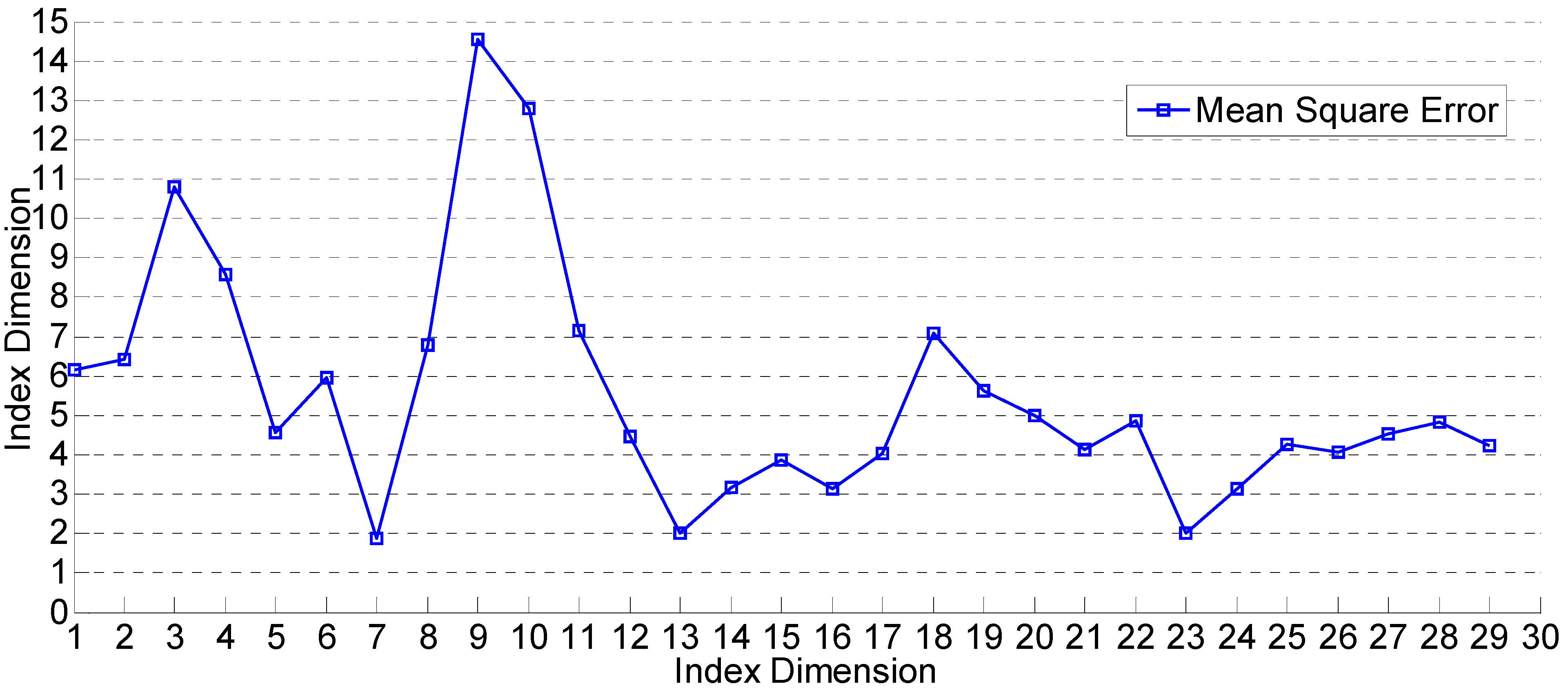
Figure 1 describes the MSE values in different indicator dimensions. It can be seen from the figure that MSE reaches the minimum when the indicator dimension is seven; as the indicator dimension increases, MSE will fluctuate heavily and then tend towards stability. Therefore, we have selected the first seven indicators, including vegetable sown acreage (X₉), material expenses’ investment (X₁), vegetable production (X₈), consumer price index (CPI) (X₂₇), rural residents’ consumption for vegetables (X₂₂), crude oil price (X₁₁) and money supply (X₂₆).

Figure 1. Mean square error (MSE) in different dimensions.

Figure 1. Mean square error (MSE) in different dimensions.

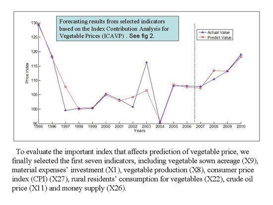
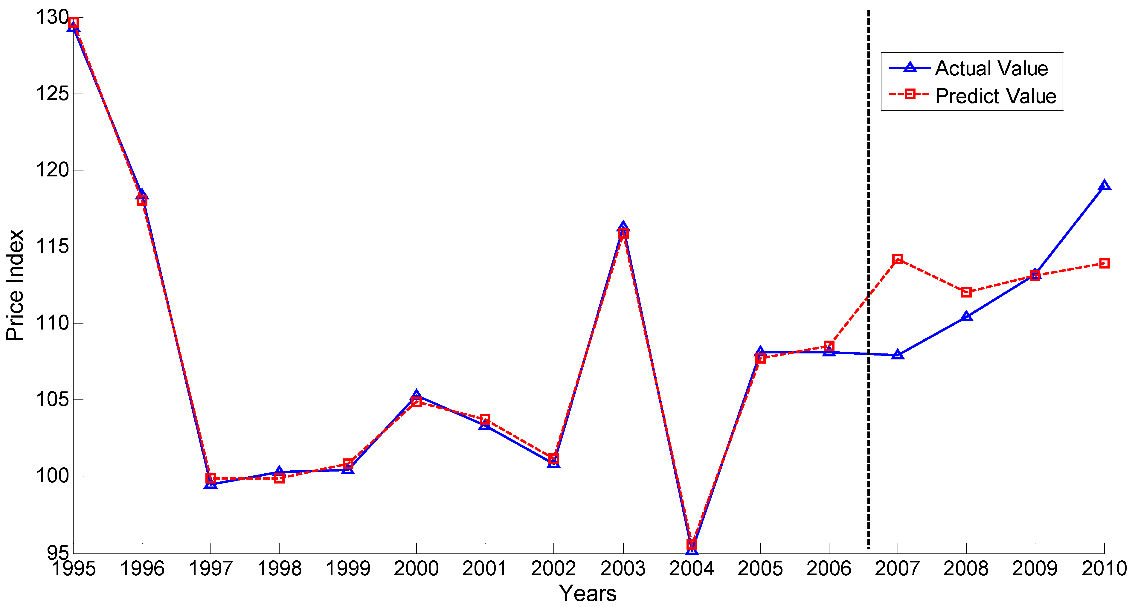
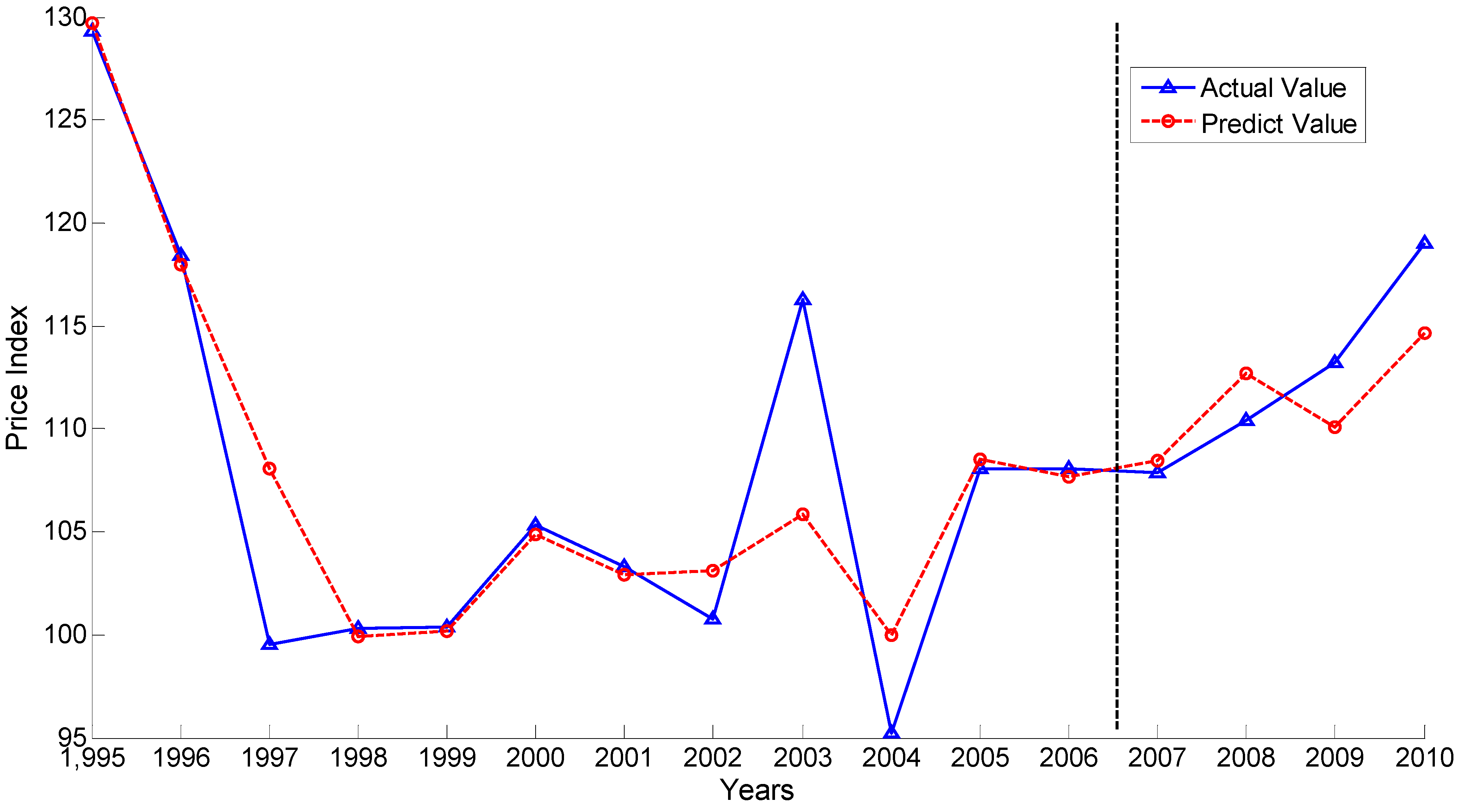
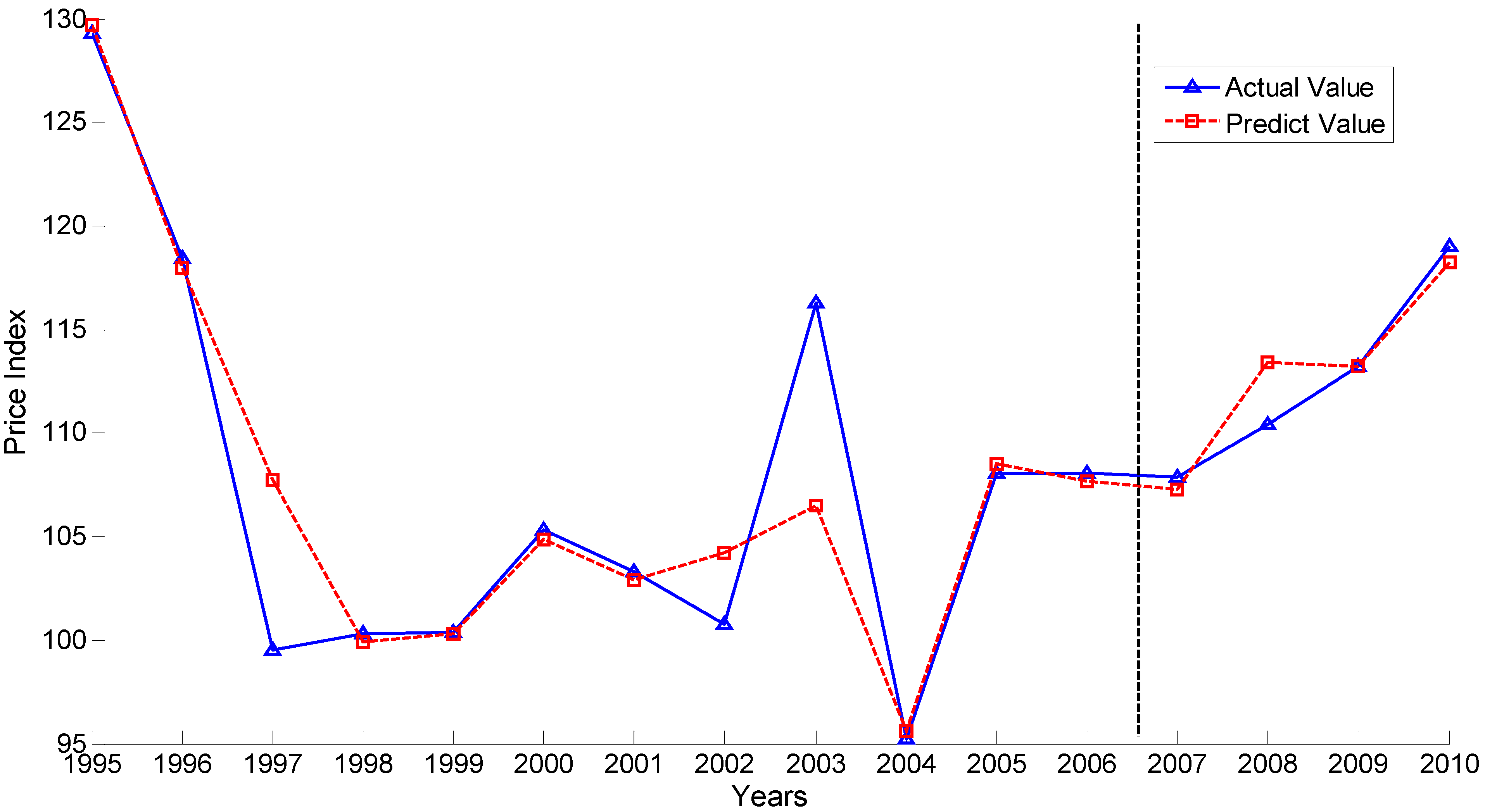
Figure 2 describes the forecasting results based on the seven indicators as the input. Figure 3 depicts the forecasting results based on the 29 indicators as the input. Through comparison of the two figures, it can be obviously found that the forecasting results of selected indicators based on the ICAVP algorithm perform better.

Figure 2. Forecasting results from selected indicators based on the index contribution analysis for vegetable prices (ICAVP).

Figure 2. Forecasting results from selected indicators based on the index contribution analysis for vegetable prices (ICAVP).

Because the other 22 indicators seldom influence the results of the early-warning system, we choose the above seven indicators (X₉, X₁, X₈, X₂₇, X₂₂, X₁₁, X₂₆) to discuss the economic rationale. From the view of economic analysis, the seven feature indicators extracted through the ICAVP algorithm have obvious relevance to the vegetable price index.

Figure 3. Forecasting results from 29 indicators as the input.

Figure 3. Forecasting results from 29 indicators as the input.

In order to fully understand the effectiveness of ICAVP, BP network methods are carried out on the same data. The result is shown in Figure 4. It is clear to show that ICAVP performs better than BP networks. Thus, the features we extracted via ICAVP contribute to the accuracy of regression and have reasonable relevance to the vegetable price index.

Figure 4. Comparative experiment design by using BP networks.

Figure 4. Comparative experiment design by using BP networks.

Vegetable sown acreage is an important factor affecting the supply of vegetables, and how large the vegetable supply is will directly affect the price of vegetables. There is a high correlation between vegetable sown acreage and vegetable production, and it can be shown that China’s vegetable sown acreage and vegetable production continues to grow year after year. The vegetable sown acreage and vegetable production in 2010 are, respectively, 3.10-times and 3.4-times those in 1990. The annual vegetable production will have accompanying changes with the volatility of vegetable sown acreage, which means the annual vegetable production will change corresponding to heavy fluctuations in the vegetable sown acreage in the next year. Overall, there exists a lagged correlation between the changes of annual vegetable production and vegetable sown acreage.

Material expenses’ investment, including seeds, pesticides, fertilizers, irrigation, machinery, tools, materials, marketing and other expenses, is an essential element supporting the growth of vegetables. The material expenses’ investment is represented by the total amount of material expenses per acre and per year. From data analysis of 1995–2010, there is a significant, increasing trend for this indicator. The material expenses’ investment has a positive relationship with vegetable production, which directly affects the production cost of vegetables, thus affecting the vegetable price.

Vegetable production changes will affect the market supply of vegetables, resulting in fluctuations in the price of vegetables. Over the years, with the rapid development of China’s vegetable industry, annual vegetable production grows year after year. China’s vegetable production increased rapidly in the 1990s, and up until 2010, the production amount increased by more than three times that in the early 1990s.

The Consumer Price Index (CPI) measures the relative ratio of residents’ consumer goods and service price level with time changes, which comprehensively reflects the changes between the living consumer goods purchased by residents and the service price levels. The vegetable prices and CPI influence each other, and there is a dialectical relationship between the two, which means, from the contribution analysis of the main agricultural products prices on CPI, the retail price index of meat, poultry and eggs and also the retail price index of fresh vegetables have the greatest impact on the Consumer Price Index.

Next is the rural residents’ demand for vegetables. China is a large agricultural country, where the number of rural residents makes up a high proportion of the population, and so, rural residents’ demand for vegetables has a significant impact on vegetable prices. Since the 1980s, rural residents’ consumption first increased, then decreased and, finally, has tended towards stability. The vegetable consumption of rural residents in 2010 was 62.62 million tons, so this huge demand has a major influence on vegetable prices.

The crude oil price has played an instrumental role in the increase of vegetable prices. According to estimates, as the crude oil price increases four percent, the vegetable sown cost will grow by three percent. In addition to increased planting costs, transportation costs also increase significantly.

The fluctuation of vegetable prices has a close relationship with domestic money supply. In the early period when the prices of China’s agricultural products rose sharply, correspondingly, there often existed a rapid growth in money supply. Money supply in circulation promotes the growth of vegetable prices. Some Chinese scholars have done research showing that when the amount of currency in circulation is increased by one trillion yuan, the prices of cabbage, cucumbers, tomatoes, green pepper and green beans will also be increased by 0.43 yuan, 0.76 yuan, 0.83 yuan, 1 yuan and 1.2 yuan per kilogram, respectively [20].

4. Conclusions

The proposed ICAVP algorithm in this paper adopts three different sampling strategies, and 15,000 tests are performed. The corresponding MSE values of 10 indicators are calculated for each sampling strategy, as well as the indicator contribution degree values, and finally, the input dimension at the minimal MSE based on the changing trend of contribution degree from 1–29 is obtained. It can be seen from the diagram that when the input dimension is seven, MSE reaches its minimum value and tends to be stable. The indicator contribution degree values are sorted, and the first seven indicators are extracted for further analysis, including vegetable sown acreage (X₉), material expenses’ investment (X₁), vegetable production (X₈), CPI(X₂₇), rural residents’ consumption of vegetables (X₂₂), crude oil price (X₁₁) and money supply (X₂₆). From an economic analysis perspective, the seven indicators keep in line with the actual operations in the vegetable market, which have a strong correlation with the vegetable price index. Finally, the selected seven indicators and all of the original 29 indicators are applied respectively to predict the results. Through comparison, the results show that the ICAVP algorithm performs better with a small prediction error and high precision. This algorithm effectively eliminates interference between indicators by removing some redundant indicators to obtain seven indicators with significant impact on the vegetable price index and with a small prediction error and high accuracy. Therefore, this algorithm can be used for feature extraction in price forecasting of other agricultural and industrial products.