Analysis of Income Inequality Based on Income Mobility for Poverty Alleviation in Rural China

Abstract

Since the reform and opening up, the Chinese economy has achieved sustained high-speed growth. However, the widening gaps in income, especially for rural China, seem to be a dark lining to these extraordinary achievements. Taking the duration of poverty into the consideration, this article analyzes the income inequality of rural per capita net income (RPCNI) based on income mobility in rural China. Analysis results showed that Gini coefficient of RPCNI declined, but that income mobility was mainly limited in the interior for low- and high-income groups. Income inequalities rose sharply within eastern and western China from 1990 to 2010. Benefiting from the developed economy, the upward mobility was universal in eastern China. The spillover effect on neighboring poor counties was feeble in western China, which directly caused long-term rich and poor. The Gini coefficient of RPCNI in central China was always at a low level, corresponding to the phenomenon of short-term rich and long-term poor. In northeastern China, the Gini coefficient sharply decreased and the large body of income mobility between non-neighboring groups was quite remarkable. The spatial pattern of intra-provincial Gini coefficient and income mobility of RPCNI has been divided by the “HU line”, which is a “geo-demographic demarcation line” discovered by Chinese population geographer HU Huanyong in 1935. In southeastern China, the characteristics of income mobility of each county depended on the distance between the county and the capital city. The spatial pattern of income mobility of RPCNI in agricultural provinces was different from that in non-agricultural provinces. According to the income inequality and income mobility, appropriate welfare and development policies was proposed to combat rural poverty at both regional and provincial scales.

1. Introduction

The Chinese economy has achieved sustained high-speed growth at a rate of nearly 10% of gross domestic production (GDP) for the past decade [1,2]. The GDP per capita in China increased from 1644 RMB in 1990 to 29,992 RMB in 2010 (The exchange rates for US$ to RMB were 1:4.7 and 1:6.8 in 1990 and 2010, respectively) [3]. If there is a dark lining to these extraordinary achievements, it is the widening income gap across the country [4]. China’s recent experience provides an excellent case to study the impacts of market-oriented reforms on income distribution and income inequality in many other countries experiencing rapid urbanization and economic transition [5,6,7,8,9].

Income inequality interacts with economic development in positive or negative ways [10]. Moderate income inequality helps to break egalitarianism, arouse enthusiasm and promote economic development. However, constantly growing income inequality reduces consumption levels and hinders economic development [5,11]. The rich, whose consumption demand have almost been met, occupy most of the wealth, while the poor have low income but relatively strong consumption demand. Under this circumstance, the consumer market is difficult to form and the economic development is extraordinarily blocked. A famous postulation on income inequality and economic development was put forward by Kuznets [12]. The postulation said that the income inequality first rises and then falls with economic development, tracing out an inverted-U-shaped curve [13]. Therefore, it is essential for the tradeoff between income inequality and economic development in different stages of economic development.

China has constantly adjusted its policies, considering the pursuit of equality and efficiency since the reform and opening up in 1978 [14]. During the 1980s and the early 1990s, the open door policy and coastal development strategy, favoring efficiency over equality, preferred the coastal areas and consequently increased the coastal–inland inequality [15,16,17]. In order to balance the development between different regions, the central government successively proposed “Western Development Strategy”, “Central Grow-Up Strategy” and “Northeastern Re-Rising Strategy” at the beginning of the 21st century [15,18]. These regional policies aimed to narrow the inter-regional income inequalities by the various means of infrastructural construction, financial support, and other preferential policies. At present, the reduction of income inequality is as important as economic development currently in China so as to avoid falling into the middle-income trap [1,19].

In recent years, serious concerns about China’s income inequality have been raised, both inside and outside China. Many previous studies have analyzed income inequality across various socio-economic perspectives [20,21,22] and spatial scales [23,24], and drawn a broad range of conclusions. The growing availability of aggregated data on provinces, counties and urban/rural regions from official publications makes it easier to carry out a long-lasting debate about the extent, dimensions, trajectory, mechanisms and consequences of geographical inequality, such as inter-regional disparity [25,26,27,28], intra-regional inequality [29], inter-provincial inequality [30,31,32,33], and urban–rural gap [34,35].

Firstly, the inter-regional inequalities between eastern China, central China and western China were commonly considered to be a long-term expansion trend, resulting from the disparity of natural conditions, economic conditions and social conditions [36]. However, the intra-regional inequalities of the above three regions gradually became highlighted with the transformation of economic development. Some researchers deem that the intra-regional income inequality of eastern China was greatest and growing, followed by that of western China, and, finally, that of central China was the smallest and decreasing. Secondly, inter-provincial inequality has also attracted the attention of some scholars, but the research has offered controversial findings which indicates the complexity and dynamism of inter-provincial income inequality [30,31]. Finally, the gap between urban and rural areas in China has become a very serious problem. Many scholars have studied the urban–rural inequality from the perspectives of income, education level, medical conditions, consumption, employment and public investment [34,37]. Recently, the research about subjective well-being and happiness of urban and rural China has been conducted [35,38]. Obviously, there have been sufficient research focusing on the geographical inequality mentioned above, drawing many meaningful conclusions.

By contrast, studies about income inequality in rural China are relatively scarce. With the growing urbanization and industrialization, the share of non-agricultural income in the overall income of agricultural households is sharply increasing in China [39]. Although the increasing non-agricultural income contributes to poverty reduction among agricultural households [40], it also increases intra-rural income inequality [41]. The increasing intra-rural income inequality deepens institutional barriers, forms social stratification and causes many social issues in China. Therefore, we think that the research on intra-rural income inequality is worth exploring. Most existing research has detected the level of intra-rural income inequality using the differentiation indices, such as Gini coefficient, Theil coefficient and Lorenz curve [42], and revealed the reasons causing poverty or income inequality through regression analysis or correlation analysis [43]. There has been no consistent recognition of the spatio-pattern of income inequality in rural China. In addition, income inequality might be caused by the disparity of conditions of education, transportation, location advantage, rural-to-urban migration [44,45], agricultural technology [46], population aging [47], and related policies such as the Key Priority Forestry Programs [48] and household registration (hukou) system. These reasons help to understand the restrictive factors for rural development, but are difficult to give the corresponding recommendations for the poverty alleviation for the population with different characteristics.

In addition, an important dimension of income inequality is its duration of poverty [49,50]. Empirical studies offer good snapshots of income inequality. However, for a better understanding of inequality, we need to know the extent of income mobility. Income mobility is the movement of an individual or group from one income level to another and measured in terms of upward mobility and downward mobility [51,52]. A given level of income inequality measured from cross-section data can arise from very different social situations. For example, a society in which a quarter of the population forms an underclass of the chronically poor will look the same as one with the same proportion of poor but different poor people in any given year. The counties with transient poverty will face different social and political challenges compared with the ones with chronic poverty, and they will require different policies to solve individual problems [53].

Rural China has experienced a far-reaching transition since the economic reforms in 1978. In this progress, rural China has been confronted with significant changes and subsequent restructuring of rural socio-economic morphology, including changes in demographic structures, employment opportunities, accessibility, income, and living standards [54,55,56,57,58]. Meanwhile, these changes have brought about a number of challenges to rural areas. In this paper, we examine income inequality in rural China combined with a degree of income mobility by the exploratory spatial data analysis (ESDA), Lorenz curve, Gini coefficient and Markov chain model. The aims of this paper are: (1) to explore the spatio-temporal pattern of rural per capita net income (RPCNI) in rural China; (2) to detect the rural income inequality at multiple scales; (3) to reveal the extent of income mobility between counties of different groups; and (4) to provide policy recommendations for poverty alleviation of different regions.

2. Data Source and Methods

2.1. Data Source

Two indices of RPCNI and rural population (RP) of 2347 counties in China, from the year 1990, 2000 and 2010, were selected in this paper. The RPCNI was used to analyze the spatio-temporal pattern of rural income and income mobility between different groups of counties in rural China. RPCNI actually consists of four parts, i.e., the income from wages and salaries, household operations, properties, and transfer payment. For China’s farmers, there is almost no statutory social welfare. The RPCNI can almost represent the welfare of farmers. Inspired by the target of building a moderately prosperous society by 2020, the poverty alleviation in rural areas has attracted much attention from the government and researchers. Currently, there are 832 poverty counties in China, which were chosen mainly according to the average RPCNI of each county. Even if there is large inequality in each county, the results based on the county-level RPCNI can meet the needs of providing policy recommendation for the regional and provincial poverty alleviation. The data of RPCNI at the county-level are from the “China statistical yearbook for regional economy” and “China county statistical yearbook” [3,59]. The RP was used to calculate the Gini Coefficient combined with RPCNI. The data of RP were derived from “Tabulation on the population census of China” in 1990, 2000 and 2010.

The study at provincial scale and regional scale used the data at county level mentioned above. In this paper, except for Taiwan, Hong Kong and Macao, the other 31 provinces in China were selected and grouped into four regions [60]. Beijing, Tianjin, Hebei, Shandong, Jiangsu, Shanghai, Zhejiang, Fujian, Guangdong and Hainan were grouped into the eastern China group. The central China group included Shanxi, Anhui, Jiangxi, Henan, Hubei and Hunan. Liaoning, Jilin and Heilongjiang were in the northeastern China group. The other provinces were grouped into western China.

2.2. Exploratory Spatial Data Analysis

Moran’s I is a classic measure for spatial autocorrelation [61]. The global Moran’s I can be used to diagnose the overall clustering of RPCNI in China and is calculated as follows:

$$I=\frac{{\displaystyle \sum _{i=1}^n{\displaystyle \sum _{j\ne i}^n{W}_{ij}\left(Y_i-\overline{Y}\right)\left(Y_j-\overline{Y}\right)}}}{S^2{\displaystyle \sum _{i=1}^n{\displaystyle \sum _{j\ne i}^n{W}_{ij}}}}$$

(1)

$$S^2=\frac{1}{n}{\displaystyle \sum _{i=1}^n{\left(Y_i-\overline{Y}\right)}^2}$$

(2)

$$\overline{Y}=\frac{1}{n}{\displaystyle \sum _{i=1}^n{Y}_i}$$

(3)

where Y_i/Y_j is the RPCNI of county i/j, $\overline{Y}$ is the average RPCNI in China, S² is variance of RPCNI in China, n is the number of counties in China, and W_ij is the Queen Contiguity weights matrix of 0 and 1, which defines a location’s neighbors as those with either a shared border or vertex. W_ij equals 1 when i and j are neighbors, otherwise W_ij equals 0 [61]. Its statistical significance can be evaluated based on a comparison to a random distribution. A zero value indicates that there is no spatial autocorrelation. Negative/Positive value means negative/positive spatial autocorrelation [62,63].

While the Moran’s I is a useful summary measure of global RPCNI, it does not allow us to identify local patterns of spatial association, i.e., whether or not there are clusters of counties with same level RPCNI around particular foci within the country. To answer this question, we use hot spot analysis to calculate the Getis-Ord Gi* for each county.

Getis-Ord Gi* is an index of method of hot spot analysis. It is used to calculate a significant degree of spatial aggregation to measure whether each feature with high (low) value is surrounded by features with either high (low) or low (high) values [64,65,66]. In this study, the method was used to detect the hot spots and cold spots of RPCNI during 1990–2010. The Getis-Ord Gi* is given as:

$$G_i^{\ast }={\displaystyle \sum _i{W}_{ij}{Y}_j}/{\displaystyle \sum _i{Y}_j} \mathrm{and} Z\left(G_i^{\ast }\right)=\left(G_i^{\ast }-E\left(G_i^{\ast }\right)\right)/\sqrt{VAR\left(G_i^{\ast }\right)}$$

(4)

where G_i* is a local spatial autocorrelation index, Z(G_i*) is a test score, and E(G_i*) and VAR(G_i*) are the expected value and the variance of $G_i^{\ast }$, respectively. For statistically significant positive (negative) z-scores, the larger (smaller) the z-scores, the more intense the clustering high (low) values [67].

2.3. Lorenz Curve and Gini Coefficient

The Lorenz curve and Gini coefficients (Gini) are the most widely used measures for detecting income inequality. The Lorenz curve is a geographical representation of the income distribution. It shows the correlation between the cumulative proportion of people on the x-axis (arrayed by the income level from the lowest to the highest) and the cumulative proportion of their corresponding income on the y-axis. The Gini coefficient is measured as twice the area bounded by the Lorenz curve and the egalitarian line which representing perfect equality with a 45° line. The steps are as follows: (1) counties are arrayed by the size of their RPCNI from lowest to highest; (2) calculate the gross farmers’ income (GFI) for each county; (3) calculate the cumulative proportion of rural population and GFI of each arrayed county; and (4) draw the Lorenz curve. The Gini coefficient is derived from the Lorenz curve [68].

$$G=1-{\displaystyle \sum \left[a\times \left(2b-c\right)\right]}$$

(5)

where G is Gini coefficient, a and c are the proportion of rural population and GFI of each county, respectively, and b is the cumulative proportion of GFI of each county. Usually, the Gini coefficient is between 0–1. If the RPCNI for each county becomes more unequal, the Gini coefficient becomes greater, and vice versa.

2.4. Markov Chains

Markov chains are probabilistic models introduced by Andrej Andreevic Markov at the beginning of the 20th century [69]. Since being introduced, capturing dependencies between successive observations of a random variable is mainly done by means of Markov chains. As a counter part to the continuous approach of the stochastic kernel, discrete-state Markov chains have been widely adopted in the study of regional convergence and inequality dynamics [70,71]. The fundamentals of Markov chain model are introduced in this section.

The RPCNI of all counties at year t were discretized into k groups. The probability distribution evolves according to the following transition probability matrix (Table 1).

Table 1. Markov transition probability matrix (k = 4).

ti/ti + 1	1	2	3	4
1	m11	m12	m13	m14
2	m21	m22	m23	m24
3	m31	m32	m33	m34
4	m41	m42	m43	m44

Table 1. Markov transition probability matrix (k = 4).

ti/ti + 1	1	2	3	4
1	m11	m12	m13	m14
2	m21	m22	m23	m24
3	m31	m32	m33	m34
4	m41	m42	m43	m44

In Table 1, m_ij specifies the probability of a county who transforms from group i in period t_i to group j in period t_i+1 and will be estimated using the following formula:

$$m_{ij}=\frac{n_{ij}}{n_i}$$

where $n_{ij}$ represents the numbers of counties which transform from group i to group j during year t_i−t_{i + 1}, and $n_i$ represents the numbers of counties of group i in year t_i.

If the counties remain in the same class during the study period, they are staying put; if the counties transform to more senior classes in the next time, they have upward mobility; otherwise they have downward mobility.

3. Results

3.1. Spatio-Temporal Pattern of RPCNI in Rural China

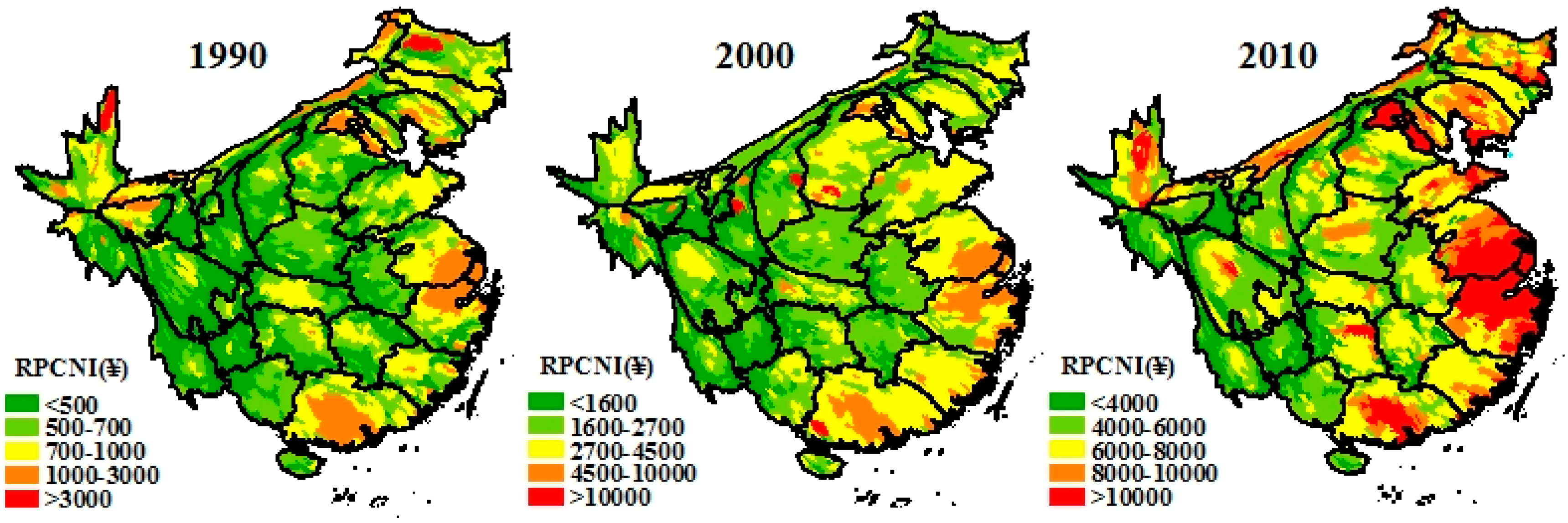
Due to the rapid economic development, the farmers’ income improved dramatically during 1990–2010. The average RPCNI of rural China increased by about 10 times, from 562 RMB to 5860 RMB during this period. Compared with their administrative border, the area of eastern counties enlarged, while that of western counties shrunk, as shown in Figure 1. Moreover, the rescaled counties had no obvious change in the three periods. The counties with high level RPCNI were mainly distributed in three growth poles (the Pearl River Delta, the Yangtze River Delta and the Bohai Rim) and spread to surrounding areas, especially in Jiangsu and Zhejiang provinces. The counties with middle level RPCNI expanded from the eastern areas to central areas. Thus, there was no doubt that the counties with low level RPCNI were more and more concentrated in western China, especially in Tibet.

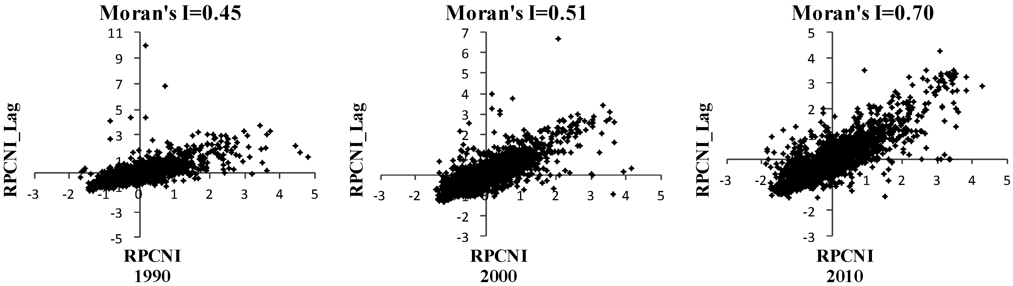
With increasingly frequent cultural and economic exchanges and large-scale migration, the spatial autocorrelation of RPCNI gradually enhanced. The Moran’s I increased from 0.45 in 1990 to 0.51 in 2000, and to 0.70 in 2010 (Figure 2). Counties with high (low) level RPCNI were surrounded by more and more counties with high (low) RPCNI.

Figure 1. Area cartograms of China with each county rescaled in proportion to its rural per capita net income (RPCNI) during 1990–2010.

Figure 1. Area cartograms of China with each county rescaled in proportion to its rural per capita net income (RPCNI) during 1990–2010.

Figure 2. The global Moran’s I of RPCNI during 1990–2010.

Figure 2. The global Moran’s I of RPCNI during 1990–2010.

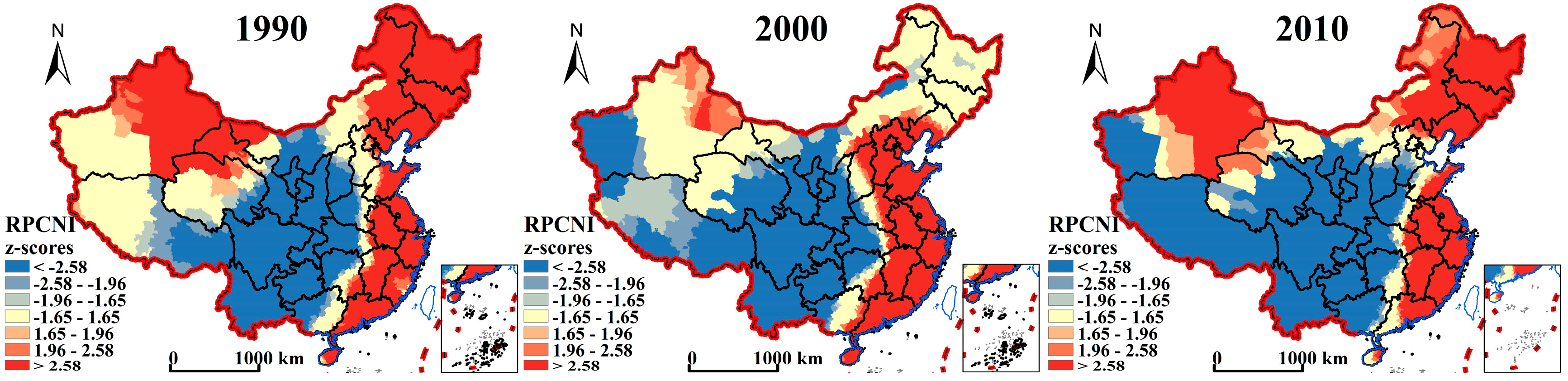
Figure 3 mapped out counties with Getis-Ord Gi* value of RPCNI for the three years: red shading for hot spots, blue shading for cold spots, and yellow shading for counties that do not exhibit statistically insignificant Gi* values. We found that significant hot spots of high RPCNI were most visible in eastern China, northeastern China and northern Xinjiang. However, the cold spots of low RPCNI were most visible in central China and western China.

Figure 3. The hot spot analysis of RPCNI in China during 1990–2010.

Figure 3. The hot spot analysis of RPCNI in China during 1990–2010.

In eastern China, along with the high-speed urbanization and industrialization, there were more opportunities for non-agricultural employment to farmers. The share of non-agricultural income increased from 32.12% to 50.15% during 1990–2010, which was far more than that of the national average level from 20.22% in 1990 to 41.07% in 2010. Furthermore, the farmers in eastern China had strong entrepreneurship and market participant ability, which made it easier for them to improve their income. The arable land per capita in northeastern China was 0.19 ha in 2010, which was higher than the national average of 0.10 ha. Benefiting from the rich arable land resource, large-scale management in agriculture was implemented and farmers’ income improved in northeastern China. In northern Xinjiang, the cash crop and animal husbandry increased the farmers’ agricultural income, while the tourism resources and the oil and gas resources were conducive to increase the non-agricultural income.

However, in central China and western China, restrained by the disadvantageous geographical location and poor infrastructure, the level of economic development of these areas lagged far behind the eastern areas. Even if there were rich energy resources, the energy industries were rarely of benefit to farmers. In addition, the education level was rather low. This increased the difficulty of popularizing agricultural science and technology and relatively decreased the employment opportunity in non-agriculture sectors for farmers with low education level. All of these resulted in the relatively lower RPCNI.

3.2. The Gini Coefficient of Overall Income Inequality in Rural China

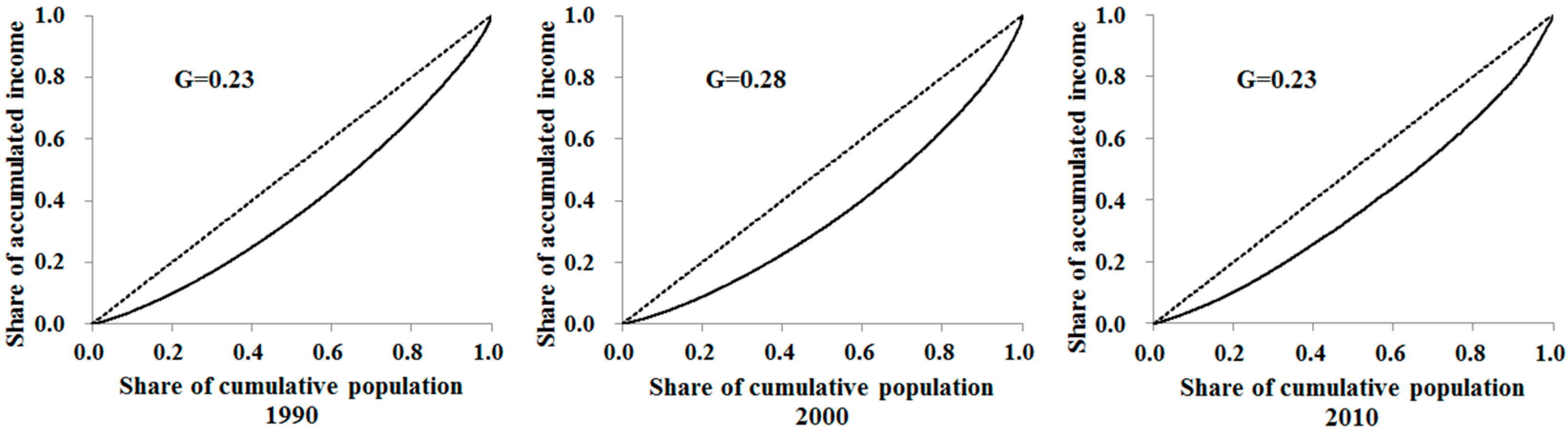
The Gini coefficient of RPCNI increased from 0.23 to 0.28 during the first decade and then decreased to 0.23 during the second decade (Figure 4). The level of income inequality in rural China increased by 21.7% during 1990–2000 but decreased by 17.9% during the last decade. To some extent, the results probably supported the inverted U-shape hypothesis, which said that in the course of a country’s development, inequality first rises before eventually declining with the growth of the level of socio-economic development. Generally speaking, the non-agricultural income due to rural-to-urban migrant was the main reason of change of income gap. During 1990–2000, the dual urban and rural household registration system loosened control. Only a small part of surplus rural labors began to migrant to urban areas and got rich, which led to the growing income inequality in rural China. During 2000–2010, the rural-to-urban migrants increased to 242 million, which accounted for 50% of farmers, and the level of urbanization increased by 13.7%. The countrywide rural-to-urban migration increased most households’ non-agricultural income, which, in turn, narrowed the income gap in rural China. The income inequality in rural China has been alleviated. However, further work needs to be done to mitigate income inequality in rural China.

Figure 4. The Lorenz curves and Gini coefficients of RPCNI in rural China during 1990–2010.

Figure 4. The Lorenz curves and Gini coefficients of RPCNI in rural China during 1990–2010.

3.3. The Gini Coefficient of Intra-Regional Income Inequality in Rural China

The overall income inequality can be divided into inter- and intra-regional income inequality. Intra-regional inequality refers to the disparity across counties in a given region. Inter-regional inequality measures the disparity between the four regions (eastern China, central China, western China and northeastern China). If the overall income inequality is higher than intra-regional income inequality, the inter-regional income inequality plays a leading role. Otherwise, the intra-regional income inequality is the main aspect of income inequality. 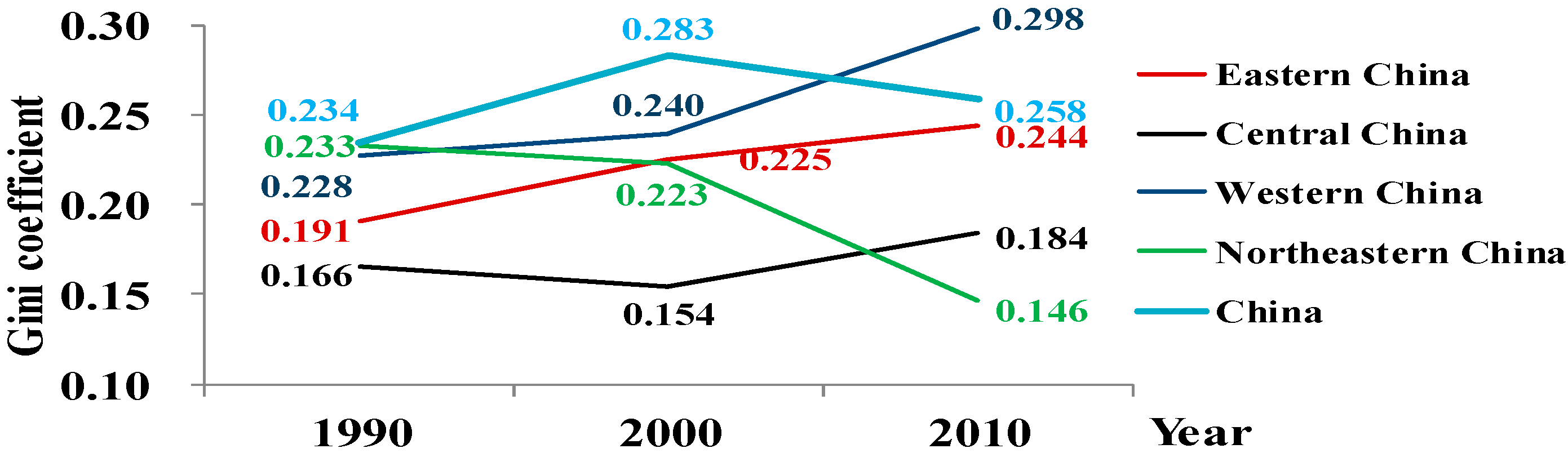As shown in Figure 5, except for the level of income inequality within western China in 2010, the levels of all other intra-regional income inequality were lower than that of overall income inequality in rural China. The results implied, even though corresponding policies for balancing regional development had been put into force, the inter-regional income inequality was still the main aspect of overall income inequality.

By contrast, the Gini coefficient rose sharply within western and eastern China but decreased greatly within northeastern China from 1990 to 2010. Specifically, the Gini coefficient in central China remained at a relatively low level and a stable state. The Gini coefficient in eastern China was always lower than that in western China but higher than that in central China (Figure 5).

Figure 5. The Gini coefficient of RPCNI in four regions of China during 1990–2010.

Figure 5. The Gini coefficient of RPCNI in four regions of China during 1990–2010.

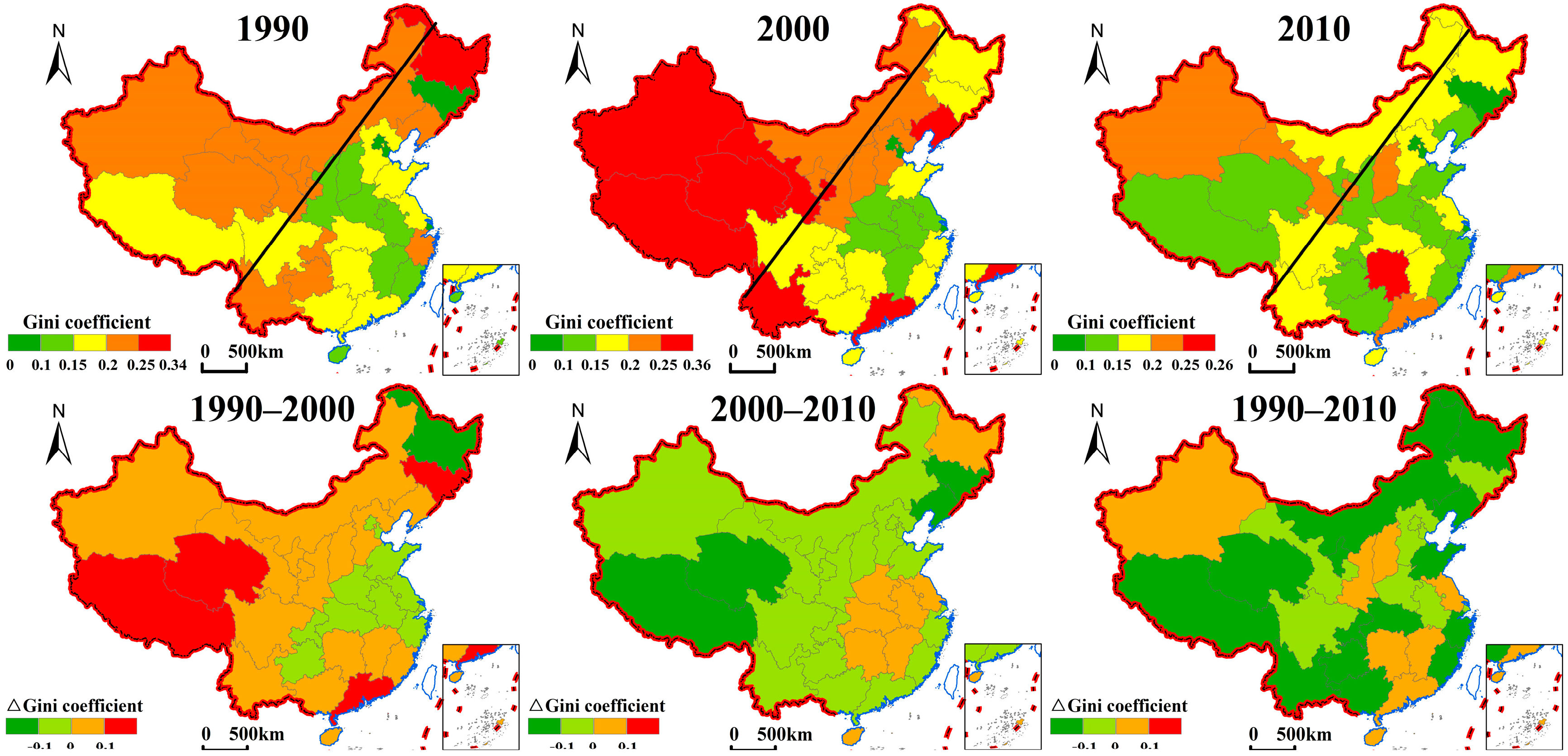
Figure 6. The Gini coefficient of intra-province income inequality in rural China during 1990–2010. The inclined line is called “HU line”.

Figure 6. The Gini coefficient of intra-province income inequality in rural China during 1990–2010. The inclined line is called “HU line”.

3.4. The Gini Coefficient of Intra-Provincial Income Inequality in Rural China

The spatial pattern of intra-provincial income inequality gradually transformed from the obvious “south–north” differentiation to a “southeast–northwest” one during the study period (Figure 6). In 1990, the northern provinces had relatively higher Gini coefficient, such as Xinjiang (0.21), Gansu (0.24), Qinghai (0.21), Inner Mongolia (0.22) and Heilongjiang (0.34). The Gini coefficients of most provinces in southern areas were prevalently less than 0.15, especially for Hainan (0.13) and Jiangxi (0.13). In 2000, the spatial pattern of intra-provincial income inequality was divided by the northeast–southwest “HU line”, which is a “geo-demographic demarcation line” discovered by Chinese population geographer HU Huanyong in 1935 [72]. The imaginary Heihe (in Heilongjiang)–Tengchong (in Yunnan) Line depicts a disparity in population distribution in China and divides the territory of China into two parts: northwest of the line covers 64% of the total area but only 4% of the population; however, southeast of the line covers 36% of the total area but 96% of the population [73]. To some extent, the “HU line” becomes the dividing line of urbanization level in China. The urbanization levels of most regions in the southeast of the line are higher than the national level. However, that of most regions in northwest of the line are lower than the national level. The discovery of the “HU line” has far-reaching implication and has become an important basis for research and decision-making. On the southeast side of “HU line”, the Gini coefficient was less than 0.2, except for Guangdong and Liaoning provinces. Conversely, the Gini coefficients of all provinces on the northwest side of “HU line” were greater than 0.2, especially Xinjiang (0.29), Qinghai (0.36), Tibet (0.26) and Yunnan (0.29). In 2010, there was no apparently spatial heterogeneity. In addition to Xinjiang, Gansu, Shanxi and Guangdong, the other provinces had low income inequality of RPCNI and the Gini coefficients were less than 0.2.

Focusing on the dynamics of Gini coefficient, the results exhibited obvious spatial heterogeneity (Figure 6). From 1990 to 2000, there was a universal increase of Gini coefficients in most provinces except for Heilongjiang and provinces in the middle and lower reaches of the Yangtze River. During 2000–2010, the Gini coefficient in most provinces declined except for Heilongjiang and the provinces in the middle and lower reaches of the Yangtze River. In view of this, the Gini coefficient of RPCNI in most provinces had successively undergone increase and decrease in the two decades, respectively, which followed the invert-U curve perfectly. Overall, the Gini coefficients of RPCNI in most provinces had decreased during 1990–2010. Under the action of the economic development policies and market mechanisms, the income inequalities at the provincial level had been narrowed successfully, which was conducive to social stability and sustainable economic development.

3.5. The Overall Income Mobility in Rural China

We used the panel data to examine the extent of income mobility by estimating Markov transition probabilities. The counties were classified into six groups with breakpoints of 60% mean income, 85% mean income, 100% mean income, 120% mean income and 150% mean income, which corresponded to the groups of the Very poor, poor, Lower-middle, Upper-middle, rich and Very rich. The groups in each year were divided according to the mean income of that year instead of the mean income of all years. We paid attention to not only the proportion of counties staying put, but also the maximum transition probability of each group which contained the upward mobility probability and downward mobility probability. In Table 2, we report Markov transition probabilities of RPCNI in rural China between 1990–2000, 2000–2010 and 1990–2010.

Table 2. Markov transition probability matrix of RPCNI in rural China (k = 6).

		Very Poor	Poor	Lower-Middle	Upper-Middle	Rich	Very Rich	No. of Counties
		<60%	<85%	<100%	<120%	<150%	>150%
1990–2000	Very poor	$\boxed{63.70}$	25.53	6.32	2.34	1.17	0.94	427
	Poor	$\begin{array}{c}33.10\end{array}$	$\boxed{33.45}$	14.98	10.80	5.75	1.92	574
	Lower-middle	13.70	$\begin{array}{c}23.62\end{array}$	$\boxed{23.32}$	22.16	14.58	2.62	343
	Upper-middle	5.32	13.16	16.20	$\boxed{28.35}$	$\begin{array}{c}27.85\end{array}$	9.11	395
	Rich	5.93	7.63	10.45	19.49	$\boxed{30.51}$	$\begin{array}{c}25.99\end{array}$	354
	Very rich	1.57	5.51	6.30	6.69	16.54	$\boxed{63.39}$	254
	No. of counties	555	475	310	346	348	313
2000–2010	Very poor	$\boxed{54.23}$	34.23	5.05	3.96	2.16	0.36	555
	Poor	16.21	$\boxed{41.26}$	$\begin{array}{c}20.42\end{array}$	18.11	3.16	0.84	475
	Lower-middle	6.13	19.03	$\boxed{25.48}$	$\begin{array}{c}34.19\end{array}$	12.90	2.26	310
	Upper-middle	2.60	5.49	14.16	$\boxed{38.44}$	$\begin{array}{c}30.64\end{array}$	8.67	346
	Rich	0.57	3.16	11.78	$\begin{array}{c}27.30\end{array}$	$\boxed{38.79}$	18.39	348
	Very rich	0.64	2.24	2.88	9.27	23.64	$\boxed{61.34}$	313
	No. of counties	410	482	303	471	382	299
1990–2010	Very poor	$\boxed{49.88}$	32.32	9.60	4.92	2.34	0.94	427
	Poor	$\begin{array}{c}22.47\end{array}$	$\boxed{35.02}$	15.33	18.47	6.45	2.26	574
	Lower-middle	11.95	19.53	$\boxed{22.45}$	$\begin{array}{c}27.41\end{array}$	15.45	3.21	343
	Upper-middle	4.30	9.37	14.43	$\boxed{32.91}$	$\begin{array}{c}29.87\end{array}$	9.11	395
	Rich	1.98	8.47	7.34	$\begin{array}{c}25.99\end{array}$	$\boxed{31.92}$	24.29	354
	Very rich	1.18	3.54	5.51	11.02	20.08	$\boxed{58.66}$	254
	No. of counties	410	482	303	471	382	299

Note: The solid line of rectangle highlight the transition probability of staying put for each group; the dotted line of rectangle highlight the maximum transition probability of upward mobility and downward mobility for each group.

Table 2. Markov transition probability matrix of RPCNI in rural China (k = 6).

		Very Poor	Poor	Lower-Middle	Upper-Middle	Rich	Very Rich	No. of Counties
		<60%	<85%	<100%	<120%	<150%	>150%
1990–2000	Very poor	$\boxed{63.70}$	25.53	6.32	2.34	1.17	0.94	427
	Poor	$\begin{array}{c}33.10\end{array}$	$\boxed{33.45}$	14.98	10.80	5.75	1.92	574
	Lower-middle	13.70	$\begin{array}{c}23.62\end{array}$	$\boxed{23.32}$	22.16	14.58	2.62	343
	Upper-middle	5.32	13.16	16.20	$\boxed{28.35}$	$\begin{array}{c}27.85\end{array}$	9.11	395
	Rich	5.93	7.63	10.45	19.49	$\boxed{30.51}$	$\begin{array}{c}25.99\end{array}$	354
	Very rich	1.57	5.51	6.30	6.69	16.54	$\boxed{63.39}$	254
	No. of counties	555	475	310	346	348	313
2000–2010	Very poor	$\boxed{54.23}$	34.23	5.05	3.96	2.16	0.36	555
	Poor	16.21	$\boxed{41.26}$	$\begin{array}{c}20.42\end{array}$	18.11	3.16	0.84	475
	Lower-middle	6.13	19.03	$\boxed{25.48}$	$\begin{array}{c}34.19\end{array}$	12.90	2.26	310
	Upper-middle	2.60	5.49	14.16	$\boxed{38.44}$	$\begin{array}{c}30.64\end{array}$	8.67	346
	Rich	0.57	3.16	11.78	$\begin{array}{c}27.30\end{array}$	$\boxed{38.79}$	18.39	348
	Very rich	0.64	2.24	2.88	9.27	23.64	$\boxed{61.34}$	313
	No. of counties	410	482	303	471	382	299
1990–2010	Very poor	$\boxed{49.88}$	32.32	9.60	4.92	2.34	0.94	427
	Poor	$\begin{array}{c}22.47\end{array}$	$\boxed{35.02}$	15.33	18.47	6.45	2.26	574
	Lower-middle	11.95	19.53	$\boxed{22.45}$	$\begin{array}{c}27.41\end{array}$	15.45	3.21	343
	Upper-middle	4.30	9.37	14.43	$\boxed{32.91}$	$\begin{array}{c}29.87\end{array}$	9.11	395
	Rich	1.98	8.47	7.34	$\begin{array}{c}25.99\end{array}$	$\boxed{31.92}$	24.29	354
	Very rich	1.18	3.54	5.51	11.02	20.08	$\boxed{58.66}$	254
	No. of counties	410	482	303	471	382	299

Note: The solid line of rectangle highlight the transition probability of staying put for each group; the dotted line of rectangle highlight the maximum transition probability of upward mobility and downward mobility for each group.

Affected by the unbalanced development strategy in China during 1990–2000, the polarization in income distribution had become serious. In total, 63.70% of the Very poor counties and 63.39% of the Very rich counties remained the same. The level of income mobility of counties in other four groups appeared relatively high. Paying attention to the maximum transition probabilities in each group, about 33.10% of the poor counties moved downward to the Very poor group and 23.62% of Lower-middle counties moved downward to poor group. Meanwhile, 27.85% of Upper-middle counties moved upward to the rich group and 25.99% of rich group moved upward to the Very rich group. It was obvious that the rich counties move upward to higher income groups and the poor counties move downward to lower income groups, which resulted in the growth of Gini coefficient in rural China from 0.23 to 0.28.

For the second decade, there was a tendency to move to the middle-income group, especially for poor group, Lower-middle group and rich group. The proportion of counties staying put in the Very poor and Very rich group were 54.23% and 61.34%, respectively, which were relatively lower than the previous decade. The maximum transition probabilities of poor, Lower-middle and Upper-middle group were 20.42%, 34.19% and 30.64%, moving up to the Lower-middle group, the Upper-middle group and the rich group, respectively. However, 27.30% of counties in rich group moved downward to the Upper-middle group. Compared with the income mobility for the first decade, the income mobility during 2000–2010 was conducive to narrowing the income gap in rural China. The results corresponded to the Gini coefficient in rural China, which decreased from 0.28 to 0.23 during the second period.

During 1990–2010, the income mobility in rural China resulted in the local equilibrium. The income mobility between the Very poor counties and poor counties was significant. Similarly, the income mobility between Lower-middle, Upper-middle and rich counties was extremely noticeable. The equilibrium was formed just within the low-income counties and high-income counties, which was in correspondence with the stable Gini coefficient of 0.23 from 1990 to 2010. The phenomenon further illustrated that it was particularly difficult for poor counties to move upward to rich counties.

Another noteworthy finding was that the income mobility usually occurred between the two neighboring groups. The proportion of income mobility between non-neighboring groups was relatively small, and the longer the distance between the two groups, the smaller the proportion was.

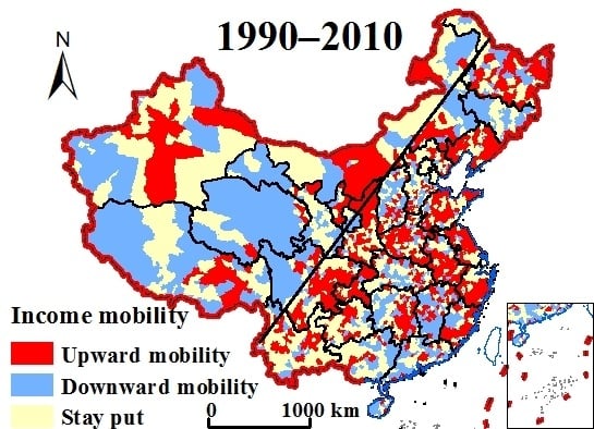
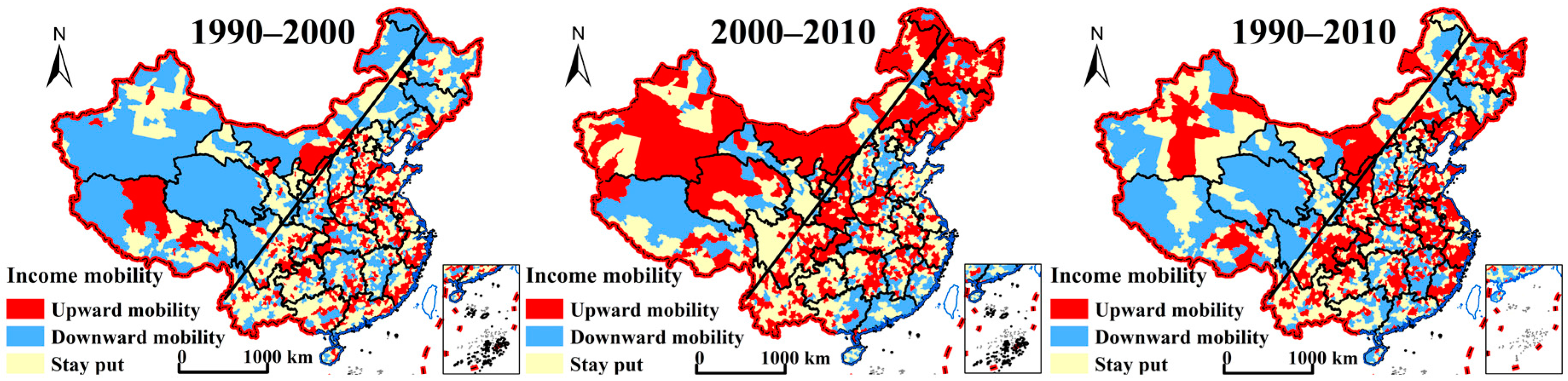
Figure 7. The income mobility in rural China at county scale during 1990–2010. The inclined line is the “HU line”.

Figure 7. The income mobility in rural China at county scale during 1990–2010. The inclined line is the “HU line”.

3.6. The Income Mobility in Rural China at County Scale

During 1990–2000, affected by the coastal development strategy and eastern development strategy, the upward income mobility tended to occur on the southeast side of “HU line” and the counties with downward income mobility mainly distributed in northeastern and western China (Figure 7). It is interesting that the counties with upward income mobility usually distributed in the inter-provincial frontier region but the counties with downward income mobility distributed in the center of provinces. This was probably due to the frequent cultural exchange and migration in the inter-provincial frontier region and the relative isolation in the central provinces.

During 2000–2010, the phenomenon of upward income mobility appeared more widespread. Benefiting from the “Western Development Strategy”, “Central Grow-Up Strategy” and “Northeastern Re-Rising Strategy”, the RPCNI of counties in the three regions had been greatly improved and the phenomenon of upward income mobility was universal. In agricultural dominated regions, such as the three northeastern provinces, Xinjiang and Inner Mongolia, the counties moving upward tended to located far from the capital city benefiting from the endowment land resources. In non-agricultural dominated regions, especially for the Yangtze River Basin, the counties moving upward usually located near the capital city, where there were more opportunities to obtain non-agricultural income owning to the developed economy. However, the counties moving downward located in Guangdong, Guangxi, Hainan and Fujian. In addition, the counties staying put mainly located in Yangtze River Basin.

As expected, the counties with upward income mobility and downward income mobility were divided by the “HU line” during 1990–2010. It is noteworthy that the counties near Urumqi and Lhasa usually moved upward. This was because the farmers there benefited much from the Urumqi’s resources-based industries and Lhasa’s tourism industries.

3.7. The Income Mobility in Rural China at Regional Scale

In order to analyze the income mobility in four regions mentioned above, we offered a range of transition probabilities matrix. Comparing the intense of income mobility with each other, we could judge the duration of poverty and propose regional policy suggestions.

Benefiting from the developed economy, the phenomenon of long-term rich was very significant in eastern China. It is noteworthy that the long-term poverty was also evident. There were about 41.33% and 74.60% counties staying put in the Very poor and the Very rich group, respectively. In addition, the maximum transition probabilities of the other four groups moving upward relied on neighboring groups (Table 3). The result proved the existence of developed counties and undeveloped counties at the same time in eastern China, such as the poverty belt around Beijing and Tianjin. Beijing and Tianjin, two municipalities directly ruled by the central government, were surrounded by 25 poverty counties resulted by the deprivation of eco-environmental resources.

Table 3. Markov transition probability matrix of RPCNI in rural China at regional scale (k = 6).

		1990–2010						No. of Counties
		Very Poor	Poor	Lower-Middle	Upper-Middle	Rich	Very Rich
Eastern China	Very poor	$\boxed{41.33}$	$\begin{array}{c}25.33\end{array}$	22.67	8.00	2.67	0.00	75
	Poor	7.41	$\boxed{43.21}$	$\begin{array}{c}32.72\end{array}$	11.11	4.94	0.62	162
	Lower-middle	3.42	13.68	$\boxed{36.75}$	$\begin{array}{c}29.06\end{array}$	10.26	6.84	117
	Upper-middle	0.00	8.26	22.31	$\boxed{28.10}$	$\begin{array}{c}26.45\end{array}$	14.88	121
	Rich	0.00	3.80	18.99	17.72	$\boxed{30.38}$	$\begin{array}{c}29.11\end{array}$	79
	Very rich	0.00	1.59	0.00	7.94	$\begin{array}{c}15.87\end{array}$	$\boxed{74.60}$	63
	No. of counties	47	119	155	111	88	97
Western China	Very poor	$\boxed{31.58}$	$\begin{array}{c}50.88\end{array}$	7.02	5.85	1.75	2.92	171
	Poor	9.36	$\boxed{41.20}$	$\begin{array}{c}23.97\end{array}$	17.98	6.37	1.12	267
	Lower-middle	10.71	$\begin{array}{c}31.43\end{array}$	$\boxed{20.71}$	17.86	15.71	3.57	140
	Upper-middle	8.33	18.06	13.89	$\boxed{24.31}$	$\begin{array}{c}29.86\end{array}$	5.56	144
	Rich	2.26	15.79	2.26	$\begin{array}{c}28.57\end{array}$	$\boxed{31.58}$	19.55	133
	Very rich	0.88	9.73	7.08	17.70	$\begin{array}{c}18.58\end{array}$	$\boxed{46.02}$	113
	No. of counties	110	299	136	176	148	99
Central China	Very poor	$\boxed{33.33}$	$\begin{array}{c}46.67\end{array}$	13.33	2.22	0.00	4.44	45
	Poor	$\begin{array}{c}27.21\end{array}$	$\boxed{34.01}$	15.65	16.33	6.12	0.68	147
	Lower-middle	13.68	$\begin{array}{c}21.37\end{array}$	$\boxed{21.37}$	$\begin{array}{c}21.37\end{array}$	19.66	2.56	117
	Upper-middle	6.57	10.22	13.14	$\boxed{33.58}$	$\begin{array}{c}29.93\end{array}$	6.57	137
	Rich	0.00	10.75	5.38	$\begin{array}{c}27.96\end{array}$	$\boxed{45.16}$	10.75	93
	Very rich	0.00	0.00	7.89	23.68	$\begin{array}{c}57.89\end{array}$	$\boxed{10.53}$	38
	No. of counties	80	120	80	131	137	29
Northeastern China	Very poor	$\boxed{27.27}$	0.00	$\begin{array}{c}50.00\end{array}$	18.18	4.55	0.00	22
	Poor	9.30	$\boxed{4.65}$	$\begin{array}{c}41.86\end{array}$	30.23	13.95	0.00	43
	Lower-middle	11.90	9.52	$\boxed{35.71}$	$\begin{array}{c}21.43\end{array}$	19.05	2.38	42
	Upper-middle	12.50	7.14	$\begin{array}{c}28.57\end{array}$	$\boxed{30.36}$	19.64	1.79	56
	Rich	0.00	8.33	$\begin{array}{c}16.67\end{array}$	$\begin{array}{c}16.67\end{array}$	$\boxed{50.00}$	8.33	12
	Very rich	10.00	0.00	20.00	10.00	$\begin{array}{c}50.00\end{array}$	$\boxed{10.00}$	10
	No. of counties	23	11	64	46	37	4

Note: The solid line of rectangle highlight the transition probability of staying put for each group; the dotted line of rectangle highlight the maximum transition probability of upward mobility and downward mobility for each group.

Table 3. Markov transition probability matrix of RPCNI in rural China at regional scale (k = 6).

		1990–2010						No. of Counties
		Very Poor	Poor	Lower-Middle	Upper-Middle	Rich	Very Rich
Eastern China	Very poor	$\boxed{41.33}$	$\begin{array}{c}25.33\end{array}$	22.67	8.00	2.67	0.00	75
	Poor	7.41	$\boxed{43.21}$	$\begin{array}{c}32.72\end{array}$	11.11	4.94	0.62	162
	Lower-middle	3.42	13.68	$\boxed{36.75}$	$\begin{array}{c}29.06\end{array}$	10.26	6.84	117
	Upper-middle	0.00	8.26	22.31	$\boxed{28.10}$	$\begin{array}{c}26.45\end{array}$	14.88	121
	Rich	0.00	3.80	18.99	17.72	$\boxed{30.38}$	$\begin{array}{c}29.11\end{array}$	79
	Very rich	0.00	1.59	0.00	7.94	$\begin{array}{c}15.87\end{array}$	$\boxed{74.60}$	63
	No. of counties	47	119	155	111	88	97
Western China	Very poor	$\boxed{31.58}$	$\begin{array}{c}50.88\end{array}$	7.02	5.85	1.75	2.92	171
	Poor	9.36	$\boxed{41.20}$	$\begin{array}{c}23.97\end{array}$	17.98	6.37	1.12	267
	Lower-middle	10.71	$\begin{array}{c}31.43\end{array}$	$\boxed{20.71}$	17.86	15.71	3.57	140
	Upper-middle	8.33	18.06	13.89	$\boxed{24.31}$	$\begin{array}{c}29.86\end{array}$	5.56	144
	Rich	2.26	15.79	2.26	$\begin{array}{c}28.57\end{array}$	$\boxed{31.58}$	19.55	133
	Very rich	0.88	9.73	7.08	17.70	$\begin{array}{c}18.58\end{array}$	$\boxed{46.02}$	113
	No. of counties	110	299	136	176	148	99
Central China	Very poor	$\boxed{33.33}$	$\begin{array}{c}46.67\end{array}$	13.33	2.22	0.00	4.44	45
	Poor	$\begin{array}{c}27.21\end{array}$	$\boxed{34.01}$	15.65	16.33	6.12	0.68	147
	Lower-middle	13.68	$\begin{array}{c}21.37\end{array}$	$\boxed{21.37}$	$\begin{array}{c}21.37\end{array}$	19.66	2.56	117
	Upper-middle	6.57	10.22	13.14	$\boxed{33.58}$	$\begin{array}{c}29.93\end{array}$	6.57	137
	Rich	0.00	10.75	5.38	$\begin{array}{c}27.96\end{array}$	$\boxed{45.16}$	10.75	93
	Very rich	0.00	0.00	7.89	23.68	$\begin{array}{c}57.89\end{array}$	$\boxed{10.53}$	38
	No. of counties	80	120	80	131	137	29
Northeastern China	Very poor	$\boxed{27.27}$	0.00	$\begin{array}{c}50.00\end{array}$	18.18	4.55	0.00	22
	Poor	9.30	$\boxed{4.65}$	$\begin{array}{c}41.86\end{array}$	30.23	13.95	0.00	43
	Lower-middle	11.90	9.52	$\boxed{35.71}$	$\begin{array}{c}21.43\end{array}$	19.05	2.38	42
	Upper-middle	12.50	7.14	$\begin{array}{c}28.57\end{array}$	$\boxed{30.36}$	19.64	1.79	56
	Rich	0.00	8.33	$\begin{array}{c}16.67\end{array}$	$\begin{array}{c}16.67\end{array}$	$\boxed{50.00}$	8.33	12
	Very rich	10.00	0.00	20.00	10.00	$\begin{array}{c}50.00\end{array}$	$\boxed{10.00}$	10
	No. of counties	23	11	64	46	37	4

Note: The solid line of rectangle highlight the transition probability of staying put for each group; the dotted line of rectangle highlight the maximum transition probability of upward mobility and downward mobility for each group.

Similar to eastern China, the long-term poverty and long-term rich resulted in the extremely high level of income inequality in western China. Moreover, income mobility mainly occurred in the interior of the three low-income groups and the other three high-income groups. The task of poverty alleviation there was arduous.

As to central China, the most prominent feature of income mobility was the long-term poor and short-term rich. Affected by the backward economy, the proportion of counties staying put in the Very poor group and the Very rich group were 33.33% and 10.53%, respectively, far less than that of eastern China and western China (Table 3). The poverty alleviation in central China is another tough issue to be tackled.

In northeastern China, the income mobility between two non-adjacent groups was widespread, especially for the counties in the Very poor groups. There were about 27.27% and 50.00% counties in the Very poor group staying put and moving upward to Lower-middle group, respectively (Table 3). The phenomenon of short-term rich is also noteworthy. There was no doubt that the level of income inequality in northeastern China decreased sharply.

4. Discussion and Conclusions

4.1. The Income Inequality and Income Mobility in Rural China

Overall, the farmers’ income improved dramatically during 1990–2010. There was significant spatial autocorrelation of RPCNI in China. The hot spots of high RPCNI concentrated in eastern China, northeastern China and northern Xinjiang. However, the cold spots of low RPCNI were most visible in central China and western China. The RPCNI decreased gradually from the coast to inland, which was consistent with the spatio-pattern of economic development in China.

Combined with the Gini coefficient and income mobility of RPCNI at the national level, we found that: (1) the increase of the Gini coefficient of RPCNI in first decade was caused by the polarization between poor counties and rich counties; however, (2) the mobility to the middle income group both from low income groups and high income groups resulted in the decrease of the Gini coefficient of RPCNI in second decade; and (3) although the Gini coefficient had declined during 1990–2010, the income mobility between counties was mainly limited in the interior of the low-income groups and high-income groups. Whether or not China has undergone the later stages of the inverted-U curve needs to be further observed.

The level of income inequalities of RPCNI rose sharply within the western and eastern China but decreased greatly within the northeastern China from 1990 to 2010. Specifically, the income inequality in central China remained relatively low level and stable. The level of income inequality in eastern China was always lower than that in western China but higher than that in central China. The conclusions confirmed again what we had already known about income inequality in rural China.

4.2. The Poverty Alleviation Policies at Regional Scale

Although the RPCNI improved universally, there was still an urgent need for poverty alleviation in rural China during the process of building a moderately prosperous society by 2020. The disparity of income inequality and income mobility at the regional scale led to different characteristics of duration of poverty. Interest in this was rooted in welfare and development policies that combated rural poverty. Generally speaking, short-term poverty can be viewed as a welfare problem, whereas long-term poverty is a development problem [51]. Only the poverty alleviation modes in line with regional characteristics can solve rural poverty in China.

In eastern China, the long-term poverty and long-term rich caused the increasing high level of income inequality there. The spillover effect of rich counties on poor counties was insufficient. There is an urgent need to propose welfare policies to narrow the gap. On the one hand, transfer payments can partly achieve the redistribution of income between rich counties and poor counties. On the other hand, the industrial transfer from rich counties to poor counties helps to create more jobs and relieve long-term poverty.

As for western China, significant income inequality should be paid more attention. According to the income mobility there, the long-term rich caused the great income gap. High-income counties were more likely to make full use of local resources to develop energy and tourism industries [74], which do not have trickle-down effects on neighboring poor counties. The key to narrowing the income gap is to make poor counties rich. Except for the traditional development-oriented poverty alleviation, policies to improve the education conditions in poor areas are extremely needed. It is useful to improve the farmers’ abilities, promote rural-to-urban migrants to find high paid jobs and, what is more, avoid intergenerational duration of poverty.

The most significant feature of central China was low level of income inequality and long-term poverty. Thus, it is not only a welfare problem, but also a development problem to mitigate rural poverty. The main task is to adopt the development-oriented poverty alleviation to ensure the rapid economic development in rural areas. Specifically, central China should adjust the industrial structure and actively undertake industrial transfer from eastern China to promote economic development and increase the RPCNI. At the same time, it is also important to improve the education conditions for farmers in central China.

In northeastern China, the sharp decline of the Gini coefficient deserves more attention. Meanwhile, the short-term rich and the income mobility between non-neighboring groups were quite remarkable in northeastern China. Thus, welfare policies are needed to combat the occasional poverty [75,76]. In consideration of the large-scale agriculture there, rural cooperative financial organizations and agricultural insurance system should be undertaken. The former could increase the agricultural investment and alleviate the shortage of agricultural production, while the latter was useful for dealing with the high risk and high loss rate of agricultural production.

4.3. The Poverty Alleviation Policies at Provincial Scale

The spatial patterns of Gini coefficient and income mobility of RPCNI at provincial scale have been divided by the “HU line”. The Gini coefficients of RPCNI in most provinces have successively increased then decreased during the two decades, following the invert-U curve perfectly. The intra-provincial income mobility of RPCNI in northwestern China was spatial heterogeneity. However, in southeastern China, this paper has drawn a broad range of interesting conclusions. Both poor counties and the counties with upward income mobility usually concentrated in the inter-provincial frontier regions. Therefore each province should undertake different development strategies and strengthen the public institutions and infrastructure construction, so as to promote economic development and increase the RPCNI there.

In addition, in agricultural dominated regions, the counties moving upward tended to located far from the capital city, while in non-agricultural dominated regions, the counties moving upward usually located near the capital cities. Thus, the non-agricultural provinces should apply preferential policies to counteract the location disadvantages of remote rural areas, whereas the agricultural provinces should pay more attention to the rural areas close to the urban center.

These findings have significant implication for poverty alleviation at regional and provincial scales in rural China. However, to help the shift from the inclusive poverty alleviation to targeted poverty alleviation, further research needs to be directed toward follow-up household surveys, so as to help people with different employment structures and family structures lift themselves out of poverty.