Article

Sustainable Trade Credit and Replenishment Policies under the Cap-And-Trade and Carbon Tax Regulations

School of Business, Tianjin University of Finance and Economics, Tianjin 300222, China
*
Author to whom correspondence should be addressed.
Sustainability 2015, 7(12), 16340-16361; https://doi.org/10.3390/su71215818
Submission received: 16 September 2015 / Revised: 27 November 2015 / Accepted: 3 December 2015 / Published: 10 December 2015
(This article belongs to the Special Issue How Better Decision-Making Helps to Improve Sustainability - Part II)

Abstract

:
The paper considers the sustainable trade credit and inventory policies with demand related to credit period and the environmental sensitivity of consumers under the carbon cap-and-trade and carbon tax regulations. First, the decision models are constructed under three cases: without regulation, carbon cap-and-trade regulation, and carbon tax regulation. The optimal solutions of the retailer in the three cases are then discussed under the exogenous and endogenous credit periods. Finally, numerical analysis is conducted to obtain conclusions. The retailer shortens the trade credit period as the environmental sensitivity of the consumer is enhanced. The cap has no effects on the credit period decisions under the carbon cap-and-trade regulation. Carbon trade price and carbon tax have negative effects on the credit period. The retailer under carbon cap-and-trade regulation is more motivated to obey regulations than that under carbon tax regulation when carbon trade price equals carbon tax. Carbon regulations have better effects on carbon emission reduction than with exogenous credit term when the retailer has the power to decide with regards credit policies.

1. Introduction

Sustainable development is the main focus of an economy. The Intergovernmental Panel on Climate Change reports that global warming is likely caused by carbon emissions [1]. Hence, many countries are implementing carbon emission regulations to reduce such emissions. One of the most effective mechanisms is the cap-and-trade mechanism. Firms under the cap-and-trade mechanism receive a free carbon emissions cap during a finite time period and can trade the cap with other firms in the same carbon trade market [2,3]. The European Union Emissions Trading system (EU ETS) is the first and largest international center that permits trade. EU ETS in China has begun to experiment with carbon emissions trading in seven provinces. Carbon tax is another carbon emissions regulation, which is a tax imposed on carbon dioxide emissions [4,5]. At present, the EU has been discussing the implementation of uniform carbon tax to compensate for the deficiency of the carbon emissions trading system implemented in January 2005 (Emission Trade System).
Moreover, enterprises in the field of carbon emission reduction have to optimize their operations to reduce carbon emissions and respond to the regulations [6,7]. Meanwhile, trade credit is widely used among enterprises for short-term financing. Here, credit is provided by the seller to the buyer, and the buyer is allowed to purchase from the seller with no immediate payment [8]. Financial Times mentioned that 90% of the global merchandise in 2007 is traded with trade credit, which is about $25 trillion [9]. Wal-Mart had $28.8 trillion accounts payable in the balance sheet in March 2009, accounting for 75% of its inventory [10]. The non-state owned enterprises in China are often offered limited support by banks; thus, they resort to trade credit as a very important financing method.
Trade credit offers retailers opportunities to stimulate demand [11], although this also tightens the latter’s capital and results in default risk. Moreover, higher demand would result in greater carbon emissions. Considering the environmental awareness of consumers regarding low carbon emissions, high carbon emissions would have a negative effect on the market demand [12]. Carbon labeling is introduced by retailers on products related to emissions (e.g., Casino in France and Tesco in Great Britain) [13]. The BBMG Conscious Consumer Report states that 51% of Americans are willing to pay more for products with high environmental quality, whereas 67% agree to purchase goods for environmental benefits [14,15]. Therefore, credit policy and carbon emissions influence consumer demand and the subsequent profits of enterprises.
Hence, revisiting the trade-off between revenue and cost of trade credit, while considering the environmental sensitivity of consumers and helping enterprises make reasonable credit and operational decisions to improve the performance and sustainability of the supply chain operation are practical management problems under the constraints of carbon emissions regulations.
Many previous studies in operation management investigated the inventory model with trade credit from the angles of cash flow and logistics coordination and on the traditional Economic Order Quantity (EOQ) model framework [16,17] by weighing capital, inventory, and fixed ordering costs. However, the analyses rarely considered the demand related to the environmental awareness of the consumers and the effects of carbon emissions regulations on the cost structure of the trade credit. The literature on the inventory model with carbon emissions regulations mostly focused on logistics optimization and has rarely discussed the effect of trade credit on cash flow. Therefore, the current paper comprehensively considers the effects of carbon emission regulations on the decisions of retailers when demand depends on credit period and carbon emissions, with the aim of exploring the optimal order and credit decisions of retailers under endogenous and exogenous trade credit periods.

2. Literature Review

The economic order quantity model of trade credit financing was first proposed by Goyal [18], which Chu et al. [19] extended to a deteriorated product. Jamal et al. [20] studied the economic production quantity (EPQ) model for manufacturers with delayed payment. Huang [17] extended Goyal’s model [18] and analyzes two-level trade credit for the first time: the credit provided by the manufacturer and the customers offered by the retailers. Teng et al. [21] studied the optimal policies of both the supplier and buyer under the non-cooperative and cooperative situations. Liao et al. [22] discussed the optimal order quantity of deteriorating product with trade credit under two storage facilities. Tsao [23] discussed the inventory policies of imperfect products.
However, the demand is constant in previous studies, which explored EPQ [24,25] or EOQ [16,17] under trade credit financing. However, in reality, market demand changes quickly and is affected by many factors (i.e., price, time, inventory level, and delayed payment period). Some scholars have realized this phenomenon so they extended the inventory mode under the condition that demand is variable. However, few studies have discussed the optimal replenishment policy of retailers under a credit period while considering consumer environmental sensitivity. Ho et al. [26] and Chung and Liao [27] studied the inventory replenishment strategy in a supply chain under trade credit financing with demand that is sensitive to price. Sarkar [28] and Teng et al. [21] established the EOQ model under trade credit financing, in which demand is dependent on time. Min et al. [29] assumed that the demand depended on the inventory level with delayed payment, whereas Soni [30] studied the optimal replenishment policy of the retailers with trade credit while considering the demand related to the price and inventory level. Su et al. [31] and Jaggi et al. [32,33] discussed the inventory models, in which demand depends on inventory level. Thangam and Uthayakumar [34] and Giri and Maiti [35] studied the trade credit financing of the product with the demand related to the price and credit period.
Trade credit can stimulate the sales; however, a longer credit period would induce increase default risk. Therefore, some authors discussed the tradeoff between increasing sales and greater default risk caused by trade credit. Lou and Wang [36] studied the optimal business credit and replenishment strategies for retailers, under the condition that market sales has a positive correlation with the business credit and a negative correlation with trade credit risk. Wu and Chan [37] and Wu et al. [38] extended the research of Lou and Wang [36] to deteriorating products. Zhang et al. [39] discussed the coordination with quantity discount contract under credit risk with stochastic demand conditions.
However, the literature above does not consider the effect on demand of the environmental awareness about carbon emissions of the consumers. Rising environmental awareness has changed consumer behavior. Researchers considered the impact of consumer environmental awareness and introduced environmental quality as a demand enhancement factor in the product demand function [40]. Glock et al. [41] assumed that demand is sensitive to price and quality. Sustainability is treated as a quality attribute and is measured in terms of the levels of scrap and emissions generated in the supply chain.
Meanwhile, the impacts of cooperative and non-cooperative behaviors between the supplier and the manufacturer have also been explored. Liu et al. [40] developed a model that includes consumer environmental awareness and competition in two stage supply chains, and adopted two-stage Stackelberg game models to investigate the dynamics between the supply chain players given three supply chain network structures. Swami Shash [42] proposed a model with a manufacturer and a retailer that coordinates the operations (i.e., wholesale price and green effort for the manufacturer and market price and green effort for the retailer). Nouira et al. [43] proposed two models. In model 1, a single product is offered by the firm, and the demand of this product depends on its greenness, while in model 2, the market is segmented between ordinary and green customers, with both demand and price depend on product greenness. The greenness of the output product is a decision variable in both models. Hovelaque and Bironneau [8] discussed the carbon-constrained EOQ model with demand that is dependent on carbon emissions and retailing price. Zhang et al. [44] discussed the impact of consumer environmental awareness of carbon emissions on order quantities and channel coordination within one manufacturer and one retailer supply chain with demand that is dependent on carbon emissions and price with two substitutable products. Du et al. [45] discussed the impact of consumers’ preference on low carbon in the emission-concerned supply chain and designed several emission-concerned contracts that can help coordinate the supply chain.
Another stream of literature that is close to the present research examines the operation decisions under carbon emissions regulations. He et al. [46] discussed carbon emissions abatement in the fashion supply chain with carbon tax regulation. Hua et al. [47] studied the optimal order quantity problems of enterprises under the deterministic demand by the EOQ model; they also considered carbon cap and trade policy only and analyzed the influences of carbon trading, trading price, and carbon caps on ordering decision, carbon emissions, and the total cost of order. The study is generalized to include the pricing decisions in Hua et al. [48]. Song and Leng [49] studied the enterprise decision-making problem of the single cycle with the stochastic demand and separately considered three types of carbon emissions restrictions (i.e., emissions, carbon tax, and carbon cap-and-trade). Arslan and Turkay [50] focused on the classical EOQ model under carbon cap, carbon taxing, carbon cap and trade regulations, and carbon offset investments in order to reduce carbon emissions. Chen et al. [51] discussed the carbon constrained EOQ in the carbon regulations, including strict carbon caps, carbon tax, cap-and-offset, and cap-and-price. Toptal et al. [11] examined joint inventory control and green investment decisions in the settings of an EOQ model under the carbon cap, cap and trade, and taxing regulations. Hovelaque and Bironneau [8] discussed the carbon constrained EOQ model with demand that is dependent on carbon emissions under the cap-and-trade regulation. Dye and Yang’s [52] work is closer to the present work as it considered the joint trade credit and inventory management with the demand dependent on the credit period with the carbon cap-and-trade policy and carbon offset policy. However, Dye and Yang did not consider the effects on demand and carbon tax regulation of the environmental sensitivity of consumers.
Considerable research on the production/inventory model with trade credit and the production/inventory model with carbon emissions regulations has been published. However, few studies combined two streams of research to discuss optimal production policies and trade credit policies with trade credit and the carbon emissions regulations. The first stream of literature assumes that demand is a function of the credit period and does not consider the effect of the environmental awareness of customers on the demand and the carbon emissions regulation on the costs incurred by enterprises. The second stream of literature assumes that demand is the function of carbon emissions and does not consider the effects of trade credit on demand and default risk. Therefore, the current paper discusses the inventory models with trade credit by incorporating the effects of carbon emissions regulations and environmental sensitivity of consumers, in order to explore optimal credit and inventory strategies.
The reminder of the paper is organized into sections. Section 3 mainly presents the notations and assumptions in the paper. Section 4 discusses the models of the enterprises profit functions in three cases: without carbon emissions regulation, carbon cap-and-trade regulation, and carbon tax regulation. Section 5 analyzes the optimal solutions in the three mechanisms under the exogenous and endogenous credit periods. Section 6 discussed the numerical analysis to illustrate the proposed model and obtain some conclusions. Section 7 presents the conclusions.

3. Notations and Assumptions

3.1. Assumptions

The following assumptions are used to establish the mathematical inventory model:
(1)
Replenishment is instantaneous; shortage is not allowed.
(2)
The retailer provides the trade credit period n to its customers.
(3)
Market demand: Demand follows the form of D ( n , Q ) = α + β n δ C Q 2 ( Q ) , where α > 0 is a scaling factor, β > 0 is a constant that governs the increasing rate of the demand with respect to the credit period, and δ > 0 reflects the demand decreasing with the carbon emissions. The carbon emission-dependent demand that is usually considered has a linear form [8]. The credit-dependent demand is used in three forms: linear, polynomial, and exponential [55]. This form of linear demand function has been used in other aspects (i.e., demand related to the price and environmental performance) [54].
(4)
The retailer would face the risk of a customers’ inability to pay off debt obligations when the retailer offers a credit period to its customers. The default risk, in which the retailer cannot receive all the receivables, is higher when the credit period offered by the retailer is longer. Three methods are used to express the increasing default risk with respect to the credit period: linear, polynomial, or exponential. The rate of the default risk given the credit period is F ( n ) = 1 e k n , where k > 0 [36,37,38].
(5)
The retailer’s opportunity cost of receivables in the provided trade credit period is e j n , where j > 0 , which refers to the interest of opportunity cost [37,38].
(6)
The retailer is assumed to be a rational man and the effect of social responsibility is not considered. Therefore, the retailer maximizes its profit to make decisions.
(7)
The decisions are made in a single period and not in multiple periods; therefore, the carbon emission cap is fixed without considering the effect of time. In addition, no big progress is seen with carbon emission reduction technology for the short period [51,52].

3.2. Notations

Several notations are used throughout this paper, and these are listed in Table 1.
Table 1. Notations in the model.
NotationsMeaning
Input parameters s Unit selling price
c Uit purchasing price of the seller
A Ordering cost of per order for the seller
h Unit holding cost for the seller, excluding interest charges
T Replenishment period for the seller
ρ Trade price of unit carbon emissions
Z Carbon emissions cap
τ Tax rate of unit carbon emission
D ( n , Q ) Market annual demand
A ^ Carbon emissions of per order for the retailer
c ^ Per unit carbon emission of purchased or produced product
h ^ Per unit carbon emission of held in inventory per unit time
OutputQReplenishment quantity for the seller, decision variable
n Trade credit period offered to the consumers by the retailer, decision variable
C Q 2 ( n , Q ) Total carbon emissions
Π 2 ( n , Q ) Annual profit of the enterprise with i = 1,2,3: 1 for no regulation, 2 for carbon cap and trade regulation, and 3 for carbon tax regulation

4. Mathematical Model

C Q 2 ( Q ) represents the annual total carbon emissions of the retailer. For the given purchasing quantity, Q , the annual replenishment times are represented by D ( n ) / Q , and the annual inventory holding cost is Q / 2 . The corresponding carbon emissions linked to the purchasing times and the inventory holding are D ( n ) A ^ / Q and Q h ^ / 2 , respectively. The amount of annual carbon emissions during the purchasing process is c ^ D ( n ) . Therefore, the amount of the total carbon emissions related to purchasing/producing, delivering, and the storing product is defined as [52].
C Q 2 ( n , Q ) = c ^ D ( n , Q ) + D ( n , Q ) A ^ / Q + Q h ^ / 2
The demand of the product in the market is mainly related to credit period and carbon emissions. The effect of carbon emissions on demand is measured in two ways: by carbon intensity, which is mainly measured by the carbon footprint [46], and by total carbon emissions, the same as Hovelaque and Bironneau [8], which is directly related to corporate social responsibility image and its brand image [8]. This paper considers the main effect of carbon emission on demand to be the total carbon emissions. Thus, the demand function is given by
D ( n , Q ) = α + β n δ C Q 2 ( Q ) = α + β n δ [ c ^ D ( n , Q ) + D ( n , Q ) A ^ / Q + Q h ^ / 2 ]
Equation (1) is substituted into Equation (2) to obtain
D ( n , Q ) = 1 2 ( 2 α 2 β n + δ Q h ^ ) Q / ( Q + δ c ^ Q + δ A ^ )
The first and second derivatives of the demand function is obtained with respect to n and Q by
D ( n , Q ) Q = δ ( Q 2 h ^ + δ Q 2 h ^ c ^ + 2 Q h ^ δ A ^ 2 α A ^ 2 β n A ^ ) 2 ( Q + δ c ^ Q + δ A ^ ) 2
2 D ( n , Q ) Q 2 = δ A ^ ( 2 β n c ^ δ + 2 α + δ 2 h ^ A ^ + 2 α c ^ δ + 2 β n ) ( Q + δ c ^ Q + δ A ^ ) 3
D ( n , Q ) n = β Q Q + δ c ^ Q + δ A ^
2 D ( n , Q ) n 2 = 0
The annual profit of the retailer without carbon emissions regulation is Π 1 ( n , Q ) . The revenue that considers default risk and opportunity cost is shown as s e ( j + k ) n D ( n , Q ) . The cost related to the purchasing process is c D ( n , Q ) + D ( n , Q ) A / Q + Q h / 2 , which consists of purchases, setups, and the inventory holding. The annual profit of the enterprise Π 1 ( n , Q ) can be expressed as
Π 1 ( n , Q ) = s e ( j + k ) n D ( n , Q ) c D ( n , Q ) D ( n , Q ) A Q Q h / 2
The annual profit of the retailer with carbon cap and trade regulation is Π 2 ( n , Q ) . Here ,   ρ [ Z C Q 2 ( Q ) ] represents the emissions cost or revenue results from the buying or selling permits. The enterprise carbon emissions are less than the carbon cap when Z C Q 2 ( Q ) 0 ; therefore, the enterprise can sell the permit to obtain the revenue. The enterprise carbon emissions are greater than the carbon cap when Z C Q 2 ( Q ) < 0 ; therefore, the enterprise can buy the permit to induce the cost. The annual profit of the enterprise Π 2 ( n , Q ) can be expressed as
Π 2 ( n , Q ) = s e ( j + k ) n D ( n , Q ) c D ( n , Q ) D ( n , Q ) A Q Q h 2 + ρ [ Z C Q 2 ( Q ) ]
The firm under carbon tax regulation is charged for each unit emission with a constant tax rate level of τ . Therefore, the annual profit of the retailer under carbon tax regulation can be expressed as
Π 3 ( n , Q ) = s e ( j + k ) n D ( n , Q ) c D ( n , Q ) D ( n , Q ) A Q Q h 2 τ C Q 2 ( Q )

5. Optimal Solutions with Exogenous Trade Credit

The trade credit period n provided by the retailer is an exogenous variable that is decided by the market. The credit period is regarded as a given parameter; thus, the decision variables in the model is Q. The objective is to maximize the profit of the retailer.

5.1. Case 1: Without Carbon Emissions Regulation

The profit function in Case 1 without carbon regulations is M a x   Π 1 ( Q ) . The optimal order quantity of the retailer is shown in Theorem 1.
Theorem 1
If s e ( j + k ) n c > 0 and A ^ > β ,   t h e n   Π 1 ( Q ) is concave with decision variable Q.
Q 1 * can be obtained from Π 1 ( Q ) Q = 0 with the condition h ^ A + h A ^ < 0 .
Proof: 
Based on Equation (8), the first-order derivative of profit function with respect to Q can be obtained as
Π 1 ( Q ) Q = s e ( j + k ) n D ( Q ) Q c D ( Q ) Q D ( Q ) Q D ( Q ) Q 2 A 1 2 h = h 2 [ 2 ( s e ( j + k ) n + c ) α δ A ^ + ( s e ( j + k ) n c ) Q 2 δ 2 h ^ c ^ + ( s e ( j + k ) n c ) Q 2 δ h ^ + 2 ( s e ( j + k ) n c ) Q δ 2 h ^ A ^ 2 ( s e ( j + k ) n c ) β n δ A ^ 2 A β n 2 A α 2 A β n c ^ δ h ^ δ 2 A A ^ 2 A α c ^ δ ] / 2 ( Q + δ c ^ Q + δ A ^ ) 2 .
The second derivative of profit function with respect to Q is
2 Π 1 ( Q ) Q 2 = ( s e ( j + k ) n c ) 2 D ( Q ) Q 2 Q 2 D ( Q ) + 2 D ( Q ) Q 2 D ( Q ) Q 3 A = [ s e ( j + k ) n δ 3 h ^ A ^ 2 c δ 3 h ^ β 2 + 2 ( s e ( j + k ) n c ) α δ 2 c ^ A ^ + 2 ( s e ( j + k ) n c ) β n δ 2 c ^ A ^ + 2 ( s e ( j + k ) n c ) α δ A ^ + 2 ( s e ( j + k ) n c ) β n δ A ^ + A δ 3 h ^ c ^ A ^ + 2 A β n δ 2 c ^ 2 + 2 A β n + 2 A α + A δ 2 h ^ A ^ + 4 A α δ c ^ + 4 A β n δ c ^ + 2 A α δ 2 c ^ 2 ] / ( Q + δ c ^ Q + δ A ^ ) 3 .
If s e ( j + k ) n c > 0 and A ^ > β , 2 Π 1 ( Q ) Q 2 < 0 can be obtained. Thus, Π 1 ( Q ) is concave on decision variable Q. The maximum value can be obtained by the condition that the first derivative equals 0; hence, the optimal quantity Q 1 * can be obtained from Π 1 ( Q ) Q = 0 .
Moreover,
Π 1 ( Q ) Q | Q = 0 = 1 2 ( 2 A β n 2 A α 2 A β n c ^ δ 2 s e k n α δ A ^ 2 s e k n β n δ A ^ h ^ δ 2 A A ^ 2 A α c ^ δ + h δ 2 A ^ 2 + 2 c β n δ A ^ 2 c α δ A ^ ) / ( δ A ^ ) 2 .
If h ^ A + h A ^ < 0 , then Π 1 ( Q ) Q | Q = 0 > 0 . lim Q Π 1 ( Q ) Q < 0 is determined easily. Based on the Mean Value Theorem Q 1 * >0 exists and is unique. Hence, Q 1 * is the optimal order quantity of the retailer. Theorem 1 is thus proven.
Based on Theorem 1, Q 1 * can be obtained from Π 1 ( Q ) Q = 0 . Let
F 1 ( Q ) = h δ 2 A ^ 2 c Q 2 δ h ^ + 2 Q 2 h δ c ^ + 2 Q h δ A ^ 2 A β n + s e ( j + k ) n Q 2 δ h ^ 2 A α + 2 c β n δ A ^ c Q 2 δ 2 h ^ c ^ 2 c Q δ 2 h ^ A ^ + 2 Q h δ 2 c ^ A ^ 2 A β n c ^ δ 2 s e ( j + k ) n α δ A ^ 2 s e ( j + k ) n β n δ A ^ + s e ( j + k ) n Q 2 δ 2 h ^ c ^ + 2 s e ( j + k ) n Q δ 2 h ^ A ^ 2 c α δ A ^ h ^ δ 2 A A ^ + Q 2 h δ 2 c ^ 2 2 A α c ^ δ Q 2 h .
Therefore, Q 1 * meets F 1 ( Q ) = 0 .
Given that
F 1 ( Q ) Q = ( s e ( j + k ) n c ) 2 Q δ 2 h ^ c ^ + ( s e ( j + k ) n c ) 2 Q δ h ^ + ( s e ( j + k ) n c ) 2 δ 2 h ^ A ^ + 4 Q h δ c ^ + 2 h δ A ^ + 2 h δ 2 c ^ A ^ + 2 Q h δ 2 c ^ 2 + 2 Q h > 0 ,
F 1 ( Q ) β = 2 A n 2 A n c ^ δ ( s e ( j + k ) n c ) 2 n δ A ^ < 0 .
Therefore, Q β = F 1 ( Q ) β / F 1 ( Q ) Q > 0 . The optimal order quantity increases with β . For the given credit period, when the sensitivity of the customers to the credit period is increasing, the demand will be greater; therefore, the retailer’s optimal order quantity is increasing.
However, given the complexity of the optimal profit and carbon emission functions of the retailer, analyzing the relationship between them and the given parameters is difficult. Therefore, this relationship is discussed in the numerical analysis.

5.2. Case 2: Carbon Cap-and-Trade Regulation

The profit function in Case 2 of carbon cap-and-trade regulation is M a x Π 2 ( Q ) . The optimal solutions are shown in Theorem 2.
Theorem 2. 
If s e ( j + k ) n c > 0 , Π 2 ( Q ) is concave function with Q , Q 2 * can be obtained from Π 2 ( Q ) Q = 0 with the condition h ^ A + h A ^ < 0.
Proof: 
The first derivative of profit function can be obtained with respect to Q
Π 2 ( Q ) Q 2 = 1 2 ( 2 s e ( j + k ) n β n δ A ^ 2 s e ( j + k ) n α δ A ^ + s e ( j + k ) n Q 2 δ 2 h ^ c ^ + 2 s e ( j + k ) n Q δ 2 h ^ A ^ + s e ( j + k ) n Q 2 δ h ^ + 2 c β n δ A ^ + Q 2 h δ 2 c ^ 2 + 2 Q h δ 2 c A ^ 2 c Q δ 2 h ^ A ^ c Q 2 δ 2 h ^ c ^ 2 A α c ^ δ 2 A β n c ^ δ c Q 2 δ h ^ + 2 Q 2 h δ c ^ + 2 Q h δ A ^ 2 A β n + 2 ρ Q h ^ δ A ^ + ρ Q 2 h ^ δ c ^ 2 A α 2 ρ A ^ α + ρ Q 2 h ^ + Q 2 h 2 ρ A ^ β n + δ 2 h A ^ 2 + 2 c α δ A ^ A δ 2 h ^ A ^ ) / ( Q + δ c ^ Q + δ A ^ ) 2 .
The second derivative of profit function with respect to Q is given by
2 Π 2 ( Q ) Q 2 = [ 2 ( s e ( j + k ) n c ) c ^ α δ 2 α + 2 ( s e ( j + k ) n c ) β n δ 2 c ^ α + A ^ δ 3 h ^ c ^ α + ( s e ( j + k ) n c ) δ 3 h ^ α 2 + 2 ( s e ( j + k ) n c ) α δ α + 2 ( s e ( j + k ) n c ) β n δ α + 2 A ^ β n δ 2 c ^ 2 + 2 ρ a α + A ^ δ 2 h ^ α + 4 A ^ α δ c ^ + 2 ρ a β n + 2 A ^ β n + 2 A ^ α + 2 ρ c ^ α δ α + 2 ρ c ^ β n δ α + 4 A ^ β n δ c ^ + ρ h ^ δ 2 α 2 + 2 A ^ α δ 2 c ^ 2 ] / ( Q + δ c ^ Q δ A ^ ) 3 .
From s e ( j + k ) n c > 0 , 2 Π 2 ( Q ) Q 2 < 0 can be obtained. Thus,   Π 2 ( Q ) is concave on decision variable Q. The maximum value can be obtained on the condition that the first derivative is equal to zero.
Moreover,
Π 2 ( Q ) Q | Q = 0 = 1 2 ( 2 s e ( j + k ) n β n δ A ^ 2 s e ( j + k ) n α δ A ^ + 2 c β n δ A ^ 2 A α c ^ δ 2 β n c ^ δ 2 A β n 2 A α 2 ρ A ^ α 2 ρ A ^ β n + δ 2 h A ^ 2 2 c α δ A ^ A δ 2 h ^ A ^ ) ( δ A ^ ) 2 .
If h ^ A + h A ^ < 0 , then Π 2 ( Q ) Q | Q = 0 > 0 .  lim Q Π 2 ( Q ) Q < 0 is easy to determine. Hence, Q 2 * >0 is the optimal order quantity of the retailer. Theorem 2 is attainable.
Based on Theorem 2, Q 2 * can be obtained from Π 2 ( Q ) Q = 0 . Let
F 2 ( Q ) = 2 s e ( j + k ) n β n δ A ^ 2 s e ( j + k ) n α δ A ^ + 2 c β n δ A ^ + Q 2 h δ 2 c ^ 2 + 2 Q h δ 2 c A ^ 2 c Q δ 2 h ^ A ^ c Q 2 δ 2 h ^ c ^ 2 A c ^ δ 2 A β n c ^ δ c Q 2 δ h ^ + 2 Q 2 h δ c ^ + 2 Q h δ A ^ 2 A β n + 2 ρ Q h ^ δ A ^ + ρ Q 2 h ^ δ c ^ 2 A α 2 ρ A ^ α + ρ Q 2 h ^ s e ( j + k ) n Q 2 δ h ^ + Q 2 h 2 ρ A ^ β n + δ 2 h A ^ 2 + s e ( j + k ) n Q 2 δ 2 h ^ c ^ + 2 s e ( j + k ) n Q δ 2 h ^ A ^ + 2 c α δ A ^ A δ 2 h ^ A ^ .
Therefore, Q 2 * meets F 2 ( Q ) = 0 .
Given that
F 2 ( Q ) Q = 2 Q h δ 2 c ^ 2 + 2 h δ 2 c A ^ 2 Q c δ h ^ + 4 h δ A ^ + 2 h δ A ^ + 2 ρ h ^ δ A ^ + 2 Q ρ h ^ δ c ^ + 2 Q ρ h ^ + 2 Q δ h ^ ( s e ( j + k ) n ) + 2 Q h + 2 Q δ 2 h ^ c ^ ( s e ( j + k ) n ) + 2 δ 2 h ^ A ^ δ 2 h ^ c ^ > 0 ,
F 2 ( Q ) β = 2 s e n δ A ^ 2 c n δ A ^ 2 A n c ^ δ 2 A n 2 A ^ n < 0 .
Therefore, Q β = F 2 ( Q ) β / F 2 ( Q ) Q > 0 . The optimal order quantity increases with   β , which means the optimal order quantity of the retailer increases when the sensitivity of the customers to the credit period increases. Numerical analysis is adopted to obtain some conclusions to determine the complexity of the effects of other parameters on the decisions.

5.3. Case 3: Carbon Tax Regulation

The profit function in Case 3 of carbon tax regulation is M a x Π 3 ( Q ) . Equations (9) and (10) clearly show that carbon tax regulation is equivalent to the carbon cap-and-trade regulation with Z = 0 ,   τ = ρ . Therefore, the optimal solutions in the Theorem 3 can be obtained similar to Case 2.
Theorem 3. If s e ( j + k ) n c > 0 , Π 3 ( Q )   is concave function with Q , Q 3 * can be obtained from Π 3 ( Q ) Q = 0 with the condition h ^ A + h A ^ < 0 .
Based on Theorem 3, the optimal order quantity increases with β .
Section 5 discusses the optimal order quantity for the enterprises when the credit period is exogenous in three cases: without carbon emission regulation, carbon cap-and-trade regulation, and carbon tax regulation. The optimal order quantity of the retailer increases when the sensitivity of the customers to the credit period increases. The optimal solutions and parameter sensitivity analyses are implemented in Section 7 to obtain some conclusions.

6. Optimal Solutions with Endogenous Trade Credit

The retailer has the power to decide its credit policies, indicating that the trade credit period n provided by the retailer is an endogenous variable. Jingdong reported that customers obtain "white" after shopping, with the longest 30 days interest-free period. “Hua Ba” for Alibaba has the shortest interest-free period for 10 days and the longest interest-free period for 41 days. Thus, the decision variables in the model are n and Q.

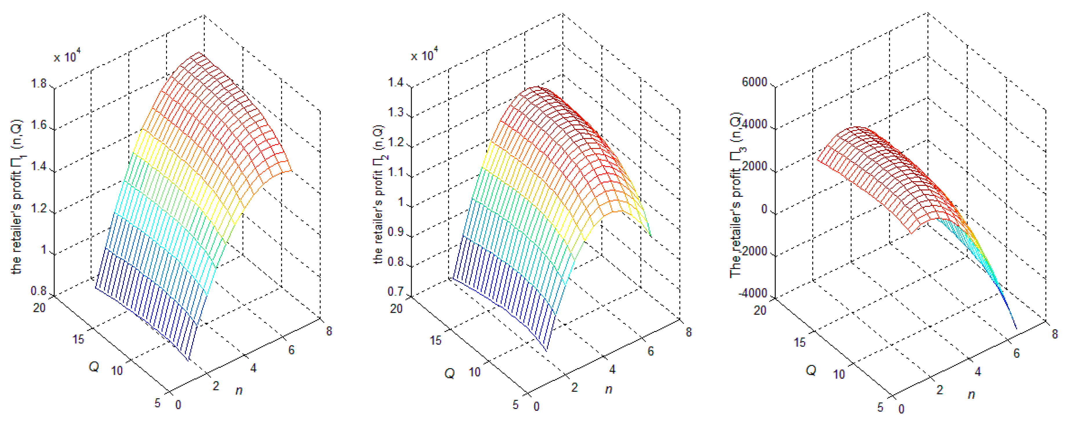
6.1. Case 1: Without Carbon Emissions Regulation

Here, n and Q are endogenous variables without the carbon emissions regulations; hence, the global optimal solution should be justified by the Hessian matrix. The Hessian matrix associated with Π 1 ( n , Q ) is given by
( 2 Π 1 ( n , Q ) n 2 Π 1 ( n , Q ) Q n Π 1 ( n , Q ) Q n 2 Π 1 ( n , Q ) Q 2 )
Owing to the complexity of the Hessian matrix, the second order conditions cannot be proven formally and obtaining the analytical solutions of n and Q is very difficult. Hence, the optimal credit period is presented on the condition that Q is a given constant.
For any given Q , the decision variable in the profit function is n. The optimal solutions are shown in Theorem 4.
Theorem 4. 
For any given Q, if   ( α + β n ) ( j + k ) ( j + k ) δ Q h ^ / 2 2 β < 0 , then
(1)
Π 1 ( n , Q )   is concave function with n .
(2)
If Π 1 ( n , Q ) n | n = 0 < 0 , then the optimal credit period n*=0.
(3)
If Π 1 ( n , Q ) n | n = 0 0, then the optimal credit period n*= n ¯ 1 .
Proof: 
Taking the first-order partial derivative of Π 1 ( n , Q )   with respect to n,
Π 1 ( n , Q ) n = 1 2 [ 2 s e ( j + k ) n ( j + k ) α Q + 2 s e ( j + k ) n ( j + k ) β n Q s e ( j + k ) n β h ^ Q 2 ( j + k ) 2 s e ( j + k ) n β Q + 2 c β Q + 2 β A ) / ( Q + δ c ^ Q + δ A ^ ] .
The second-order partial derivative of Π 1 ( n , Q ) with respect to n is
2 Π 1 ( n , Q ) n 2 = 1 2 s ( j + k ) e ( j + k ) n Q [ 2 ( j + k ) α + 2 ( j + k ) β n ( j + k ) δ Q h ^ 4 β ] / ( Q + δ c ^ Q + δ A ^ ) .
If 2 ( j + k ) α + 2 ( j + k ) β n ( j + k ) δ Q h ^ 4 β < 0 , then 2 Π 1 ( n , Q ) n 2 < 0   .   lim n Π 1 ( n , Q ) n < 0 ,  lim n Π 1 ( n , Q ) n > 0 is easy to prove. Therefore, the optimal solution n ¯ 1 exists and meets Π 1 ( n , Q ) n =0.
To justify whether n ¯ 1 is bigger than zero,
Π 1 ( n , Q ) n | n = 0 = 1 2 [ 2 s ( j + k ) α Q + 2 s ( j + k ) β n Q s β h ^ Q 2 ( j + k ) 2 s β Q + 2 c β Q + 2 β A ) / ( Q    + δ c ^ Q + δ A ^ ]
If   Π 1 ( n , Q ) n | n = 0 < 0 , then the optimal credit period n*=0. If   Π 1 ( n , Q ) n | n = 0 0, then the optimal credit period n*= n ¯ 1 .

6.2. Case 2: Carbon Cap-and-Trade Regulation

For any given Q, the decision variable in the profit function is n. The optimal solutions are obtained in Theorem 5.
Theorem 5. 
For any given Q, if   ( j + k ) ( α + β n ) β 1 2 ( j + k ) Q δ h ^ < 0 , then
(1)
Π 2 ( n , Q ) is concave function with n .
(2)
If Π 2 ( n , Q ) n | n = 0 < 0 , then the optimal credit period n*=0.
(3)
If   Π 2 ( n , Q ) n | n = 0 0, then the optimal credit period n*= n ¯ 2 .
Proof: 
Taking the first-order partial derivative of Π 2 ( n , Q ) with respect to n,
Π 2 ( n , Q ) n = ( s ( j + k ) e ( j + k ) n Q α s ( j + k ) e ( j + k ) n Q β n + s e ( j + k ) n Q β + 1 2 s ( j + k ) e ( j + k ) n Q 2 δ h ^ c Q β A β ρ c ^ Q β ρ A ^ β ) / ( Q + δ c ^ Q + δ A ^ ) .
The second-order partial derivative of Π 2 ( n , Q ) with respect to n is
2 Π 2 ( n , Q ) n 2 = ( j + k ) s e ( j + k ) n Q [ ( j + k ) α + ( j + k ) β n 2 β 1 2 ( j + k ) Q δ h ^ ] / ( Q + δ c ^ Q + δ A ^ ) .
If ( j + k ) α + ( j + k ) β n 2 β 1 2 ( j + k ) Q δ h ^ < 0 , then
2 Π 2 ( n , Q ) n < 0.    lim n Π 2 ( n , Q ) n < 0 , lim n Π 2 ( n , Q ) n > 0 is easy to prove. Therefore, the optimal solution n ¯ 2 exists and meets Π 2 ( n , Q ) n =0.
To justify whether n ¯ 2 is bigger than zero,
Π 2 ( n , Q ) n | n = 0 = ( s ( j + k ) Q α + s Q β + 1 2 s ( j + k ) Q 2 δ h ^ c Q β A β ρ c ^ Q β ρ A ^ β ) / ( Q + δ c ^ Q + δ A ^ ) / ( Q + δ c ^ Q + δ A ^ )
If Π 2 ( n , Q ) n | n = 0 <0, then the optimal credit period is n*=0. If Π 2 ( n , Q ) n | n = 0 0, then the optimal credit period is n*= n ¯ 2 .

6.3. Case 3: Carbon Tax Regulation

We discuss the optimal strategy of the retailer with carbon tax regulation when Q is a given constant. Similar to the carbon cap-and-trade regulation, Theorem 6 can be easily obtained.
Theorem 6. 
For any given Q, if   ( j + k ) ( α + β n ) β 1 2 ( j + k ) Q τ h ^ < 0 , then
(1)
Π 3 ( n , Q ) is concave function with n .
(2)
If Π 3 ( n , Q ) n | n = 0 < 0 , then the optimal credit period n*=0.
(3)
If Π 3 ( n , Q ) n | n = 0 0, then the optimal credit period n*= n ¯ 3 .
Section 6 mainly discusses the optimal decisions for the credit period and the order quantity in three cases. However, obtaining the analytical solutions of n and Q is difficult. Hence, the optimal credit period is analyzed when Q is a given constant. The optimal global solutions for credit period and order quantity are discussed by numerical analysis in Section 7.

7. Numerical Analysis

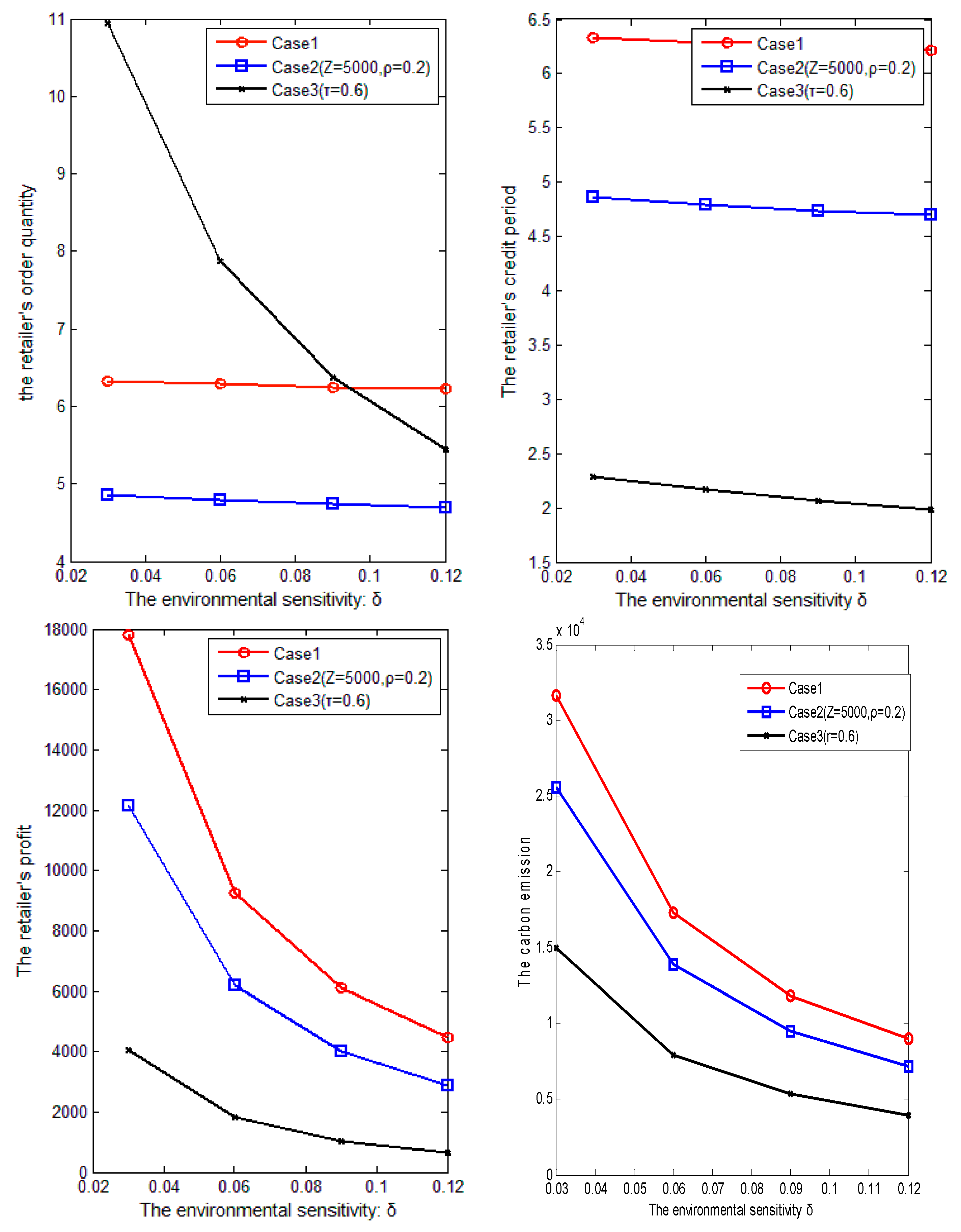
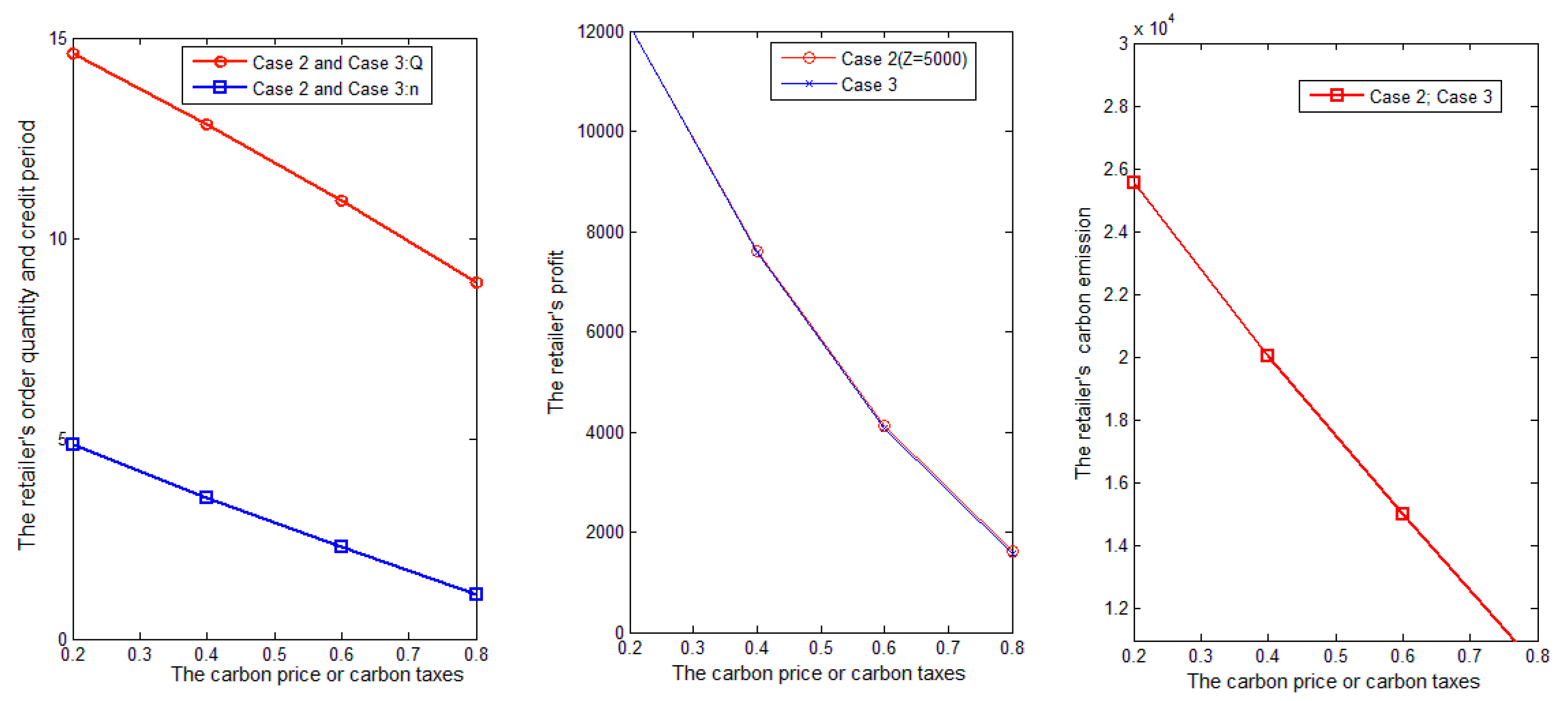
7.1. Sensitivity Analysis of One Parameter

Matlab 7.0 is used to conduct a numerical analysis with the aim of determining the effects of parameters on the optimal decision with exogenous and endogenous credit periods. The basic parameters in the models are evaluated to meet the prerequisites of the theorems for the optimal solutions: α = 200 units, β = 200 ,    δ = 0.03 ,    s = 340 $ , A = 80$ per order, c = 150$ per unit, h = 105$ per unit per month, k = 0.05, j = 0, Z = 5000 kg per month, ρ = 0.2, A ^   =   50 , c ^ = 150 ,     h ^ = 100 ,   τ = 0.6, and n = 2 months.

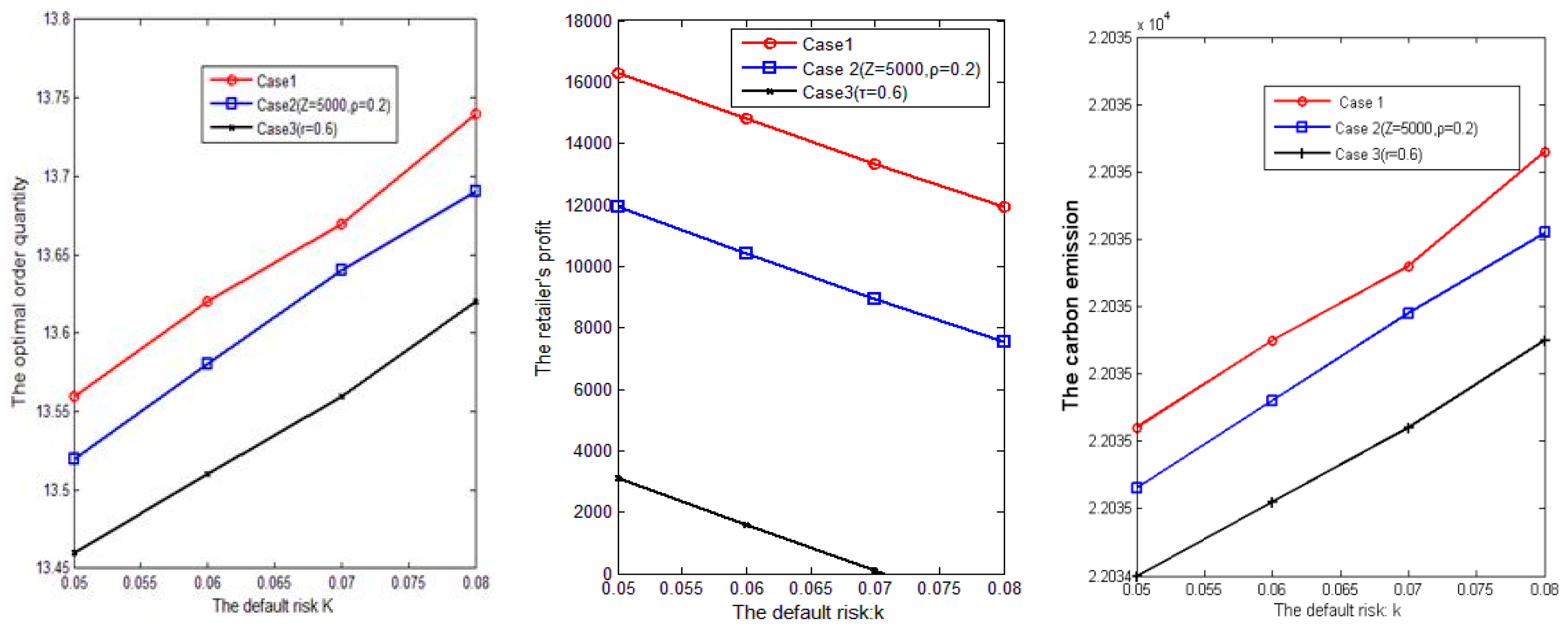
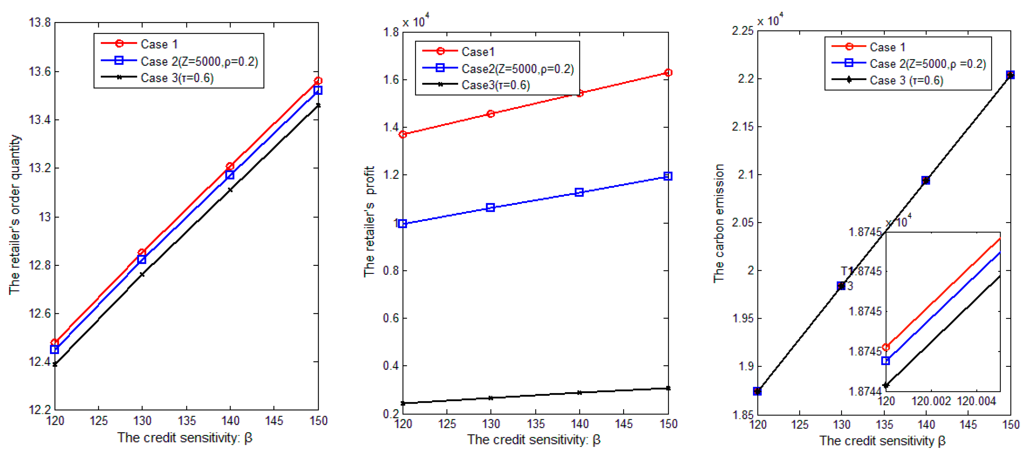
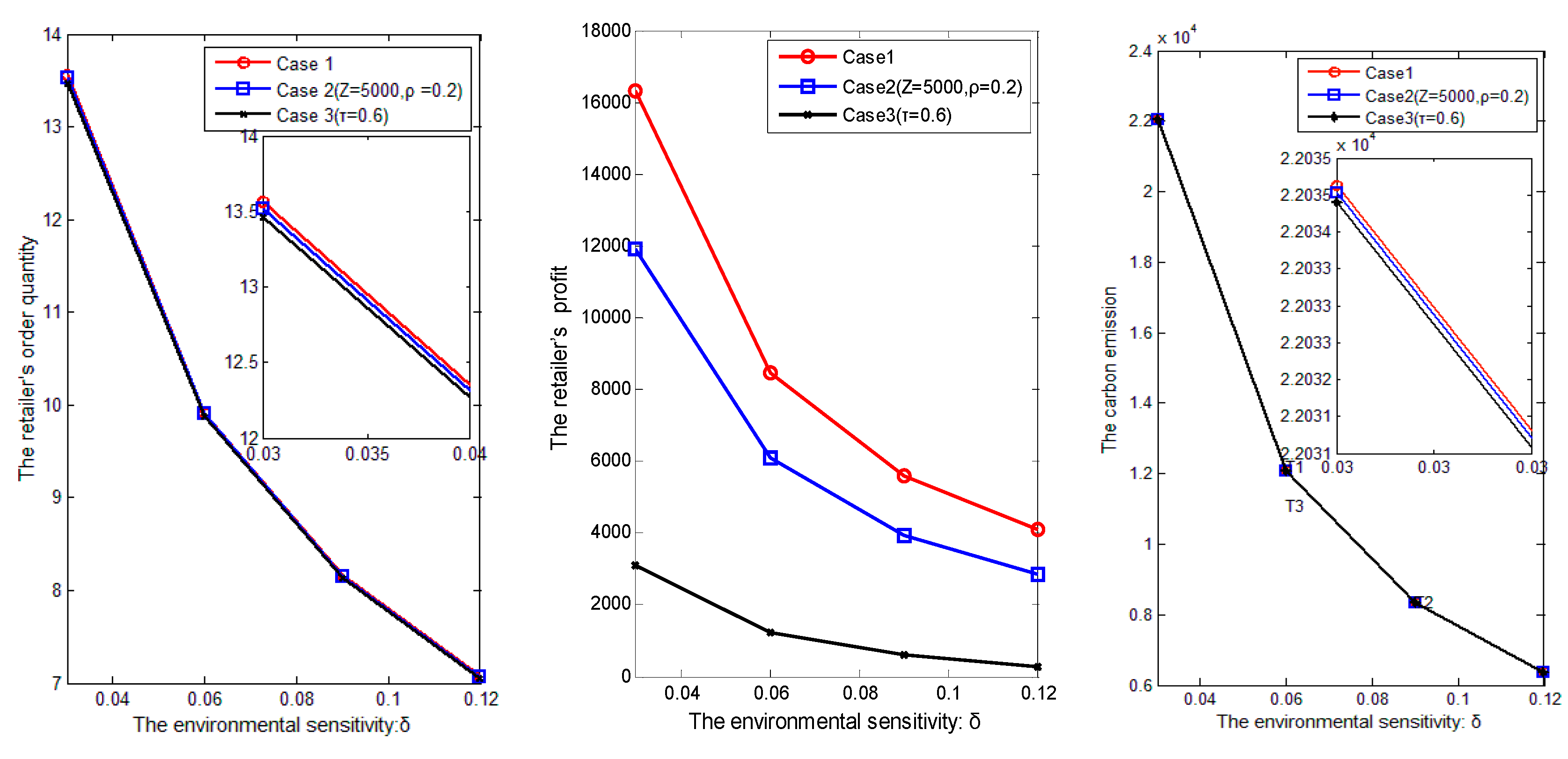
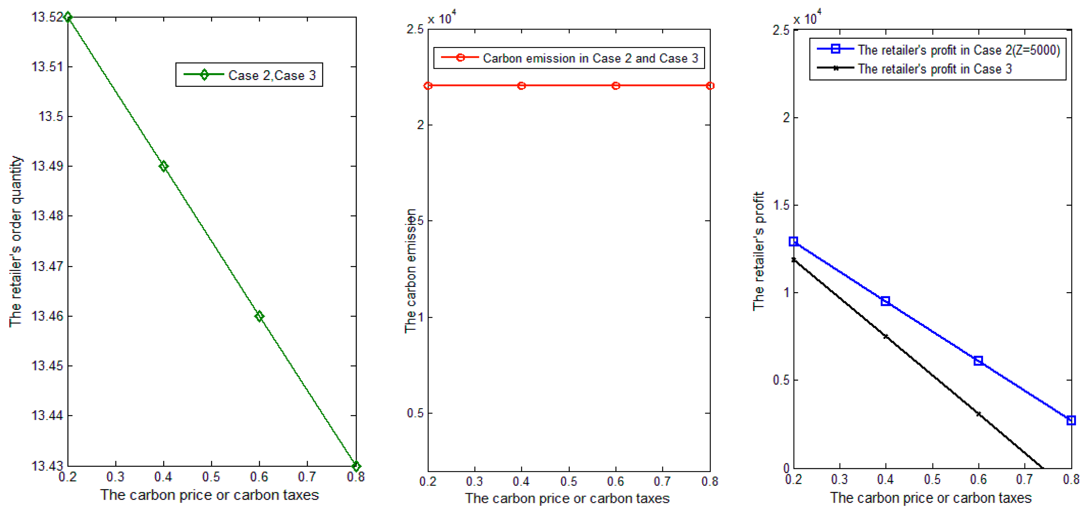
7.1.1. Exogenous Credit Period

The sensitivity analysis of parameters is conducted in the three cases with exogenous credit period. The values of the parameters meet the conditions s e ( j + k ) n c > 0 , h ^ A + h A ^ < 0 . Hence, applying Theorems 1–3, the profit functions Π 1 ( Q ) ,   Π 2 ( Q ) ,   a n d   Π 3 ( Q ) are concave with Q , respectively (Figure 1). Therefore, the following optimal order quantities can be obtained: Q 1 * = 13.56 , Q 2 * =   13.52 , and Q 3 * = 13.46 .
Figure 1. Π 1 ( Q ) , Π 2 ( Q ) ,   a n d   Π 3 ( Q ) are concave with Q .
Sustainability 07 15818 g001
Figure 2, Figure 3, Figure 4, Figure 5, Figure 6 and Figure 7 show the results of the analyses. After conducting the sensitivity analyses, the following results are obtained.
(1) Figure 2 shows that the optimal order quantity and the carbon emissions of the retailer increase and the profit decreases with the increase of credit risk k (i.e., the increase of bad debts rate). This means that the credit risk induces high carbon emissions and reduces profit, which are bad for society and the overall profit of the firm. Hence, the government and the firm should adopt some measures to reduce the credit risk and improve operational sustainability.
(2) Figure 3 shows that the optimal profit, order quantity, and carbon emissions of the retailer all increase with the increase of parameter β for the customers who are more sensitive to the credit period. The market demand is higher when credit sensitivity increases. That is because when the consumers’ credit sensitivity increasing, for the fixed credit period, it will result in higher market demand. Hence, the retailer will increase the order quantity to meet the market demand and earn more profits.
(3) Figure 4 shows that the optimal order quantity, corresponding profit, and carbon emissions of the retailer all decrease with the increase of impact factor δ of carbon emissions to the demand, suggesting increasing customer awareness of environmental protection. As long as the enterprise goes for production, it will result in carbon emission. For exogenous credit period, without considering the effect of other enterprises’ carbon emission, as the consumers’ environmental sensitivity increasing, it will induce lower market demand. Hence, the retailer will reduce the order quantity and make less profit. This can also be demonstrated in Figure 9. Therefore, consumer awareness of environmental protection helps reduce carbon emissions. The government should publicize low carbon from a variety of sources to raise consumer awareness of low-carbon environment.
(4) Figure 5 shows that the carbon emissions cap under the carbon cap-and-trade policy has no effect on the optimal decisions of the retailer. Since the retailer can buy or sell the carbon emission through the carbon trading market at a fixed price, varying the carbon cap has no effect on the optimal solutions. Based on the profit functions, it is easy to find that the carbon cap had no effect on the decisions. The conclusions can also be found in Dye and Yang [52]. However, the optimal profit increases as the carbon emissions cap increases. Hence, adjusting carbon cap to reward the carbon emissions behavior of a firm is not a good strategy.
(5) Figure 6 shows that the optimal order quantity, carbon emissions, and optimal profit of the retailer decrease as carbon trade price or carbon taxes increase. As the carbon trade price or carbon taxes increases, it will result in higher carbon emission related cost, such as the carbon emission from the holding inventory. Hence, the retailer will decrease the order quantity to accelerate the inventory turnover to reduce the inventory cost. This means that the government’s adjustment of trade price or carbon taxes to induce reduction of carbon emissions among firms is effective. When carbon trade price is equal to carbon taxes, the profit of the retailer under the carbon cap-and-trade regulation is larger than that under carbon tax regulation, but carbon emissions in both kinds of conditions are equal. Therefore, the retailer under carbon cap-and-trade regulation wherein carbon trade price is equal to carbon taxes has more incentives to obey the regulations than that under carbon tax regulation. The effect of carbon taxes on the profit of the retailer is greater than that under carbon cap and trade regulation, indicating that carbon cap lessens the effect of carbon price on profit.
Figure 2. Impacts of default risk k.
Sustainability 07 15818 g002
Figure 3. Impacts of credit sensitivity β
Sustainability 07 15818 g003
Figure 4. Impacts of environmental sensitivity δ
Sustainability 07 15818 g004
Figure 5. Case 2: Impacts of carbon Cap Z.
Sustainability 07 15818 g005
Figure 6. Impacts of carbon trade price or carbon taxes.
Sustainability 07 15818 g006
Figure 7. Π 1 ( n , Q ) , Π 2 ( n , Q ) ,   a n d   Π 3 ( n , Q ) changing with n and Q.
Sustainability 07 15818 g007

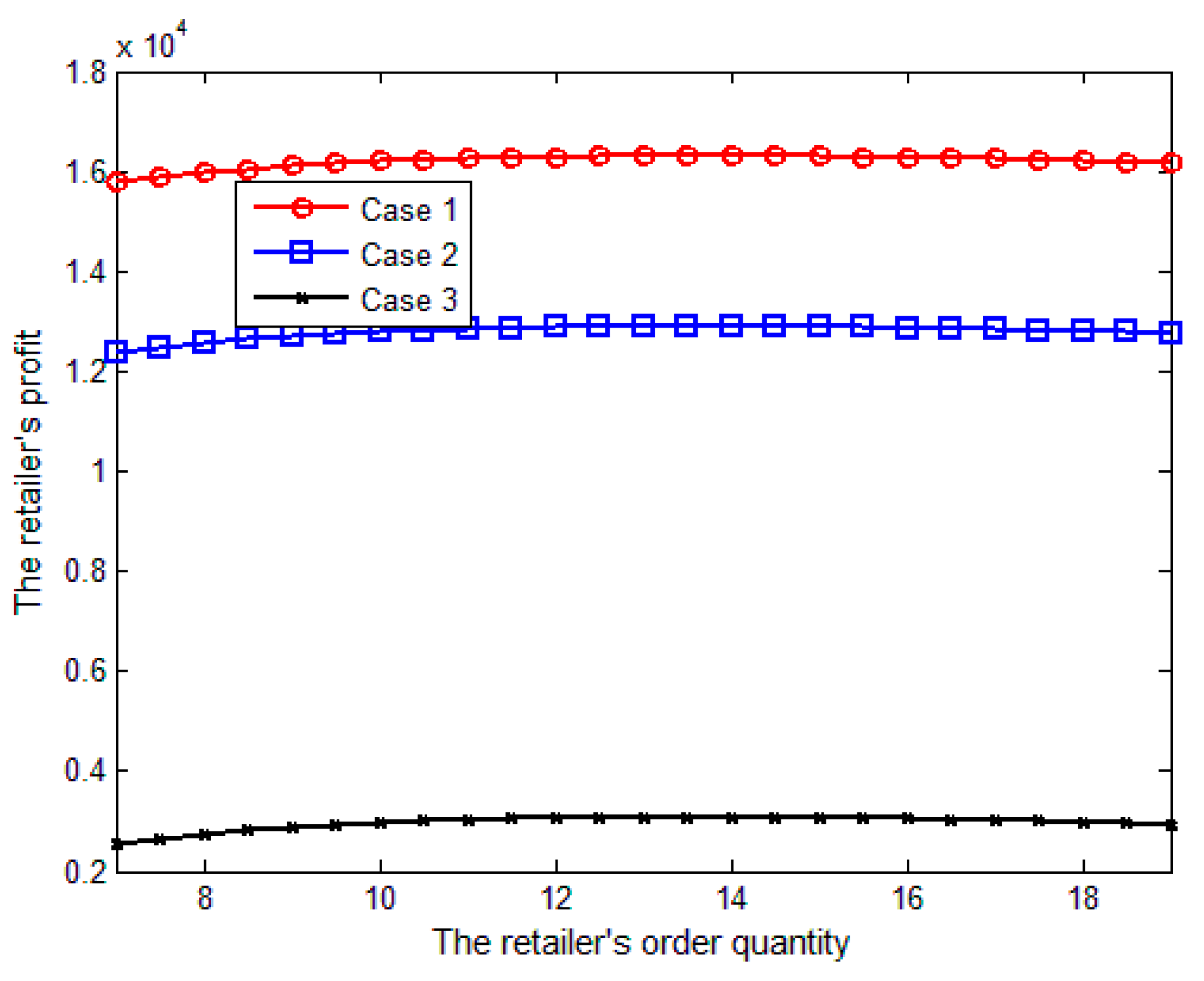
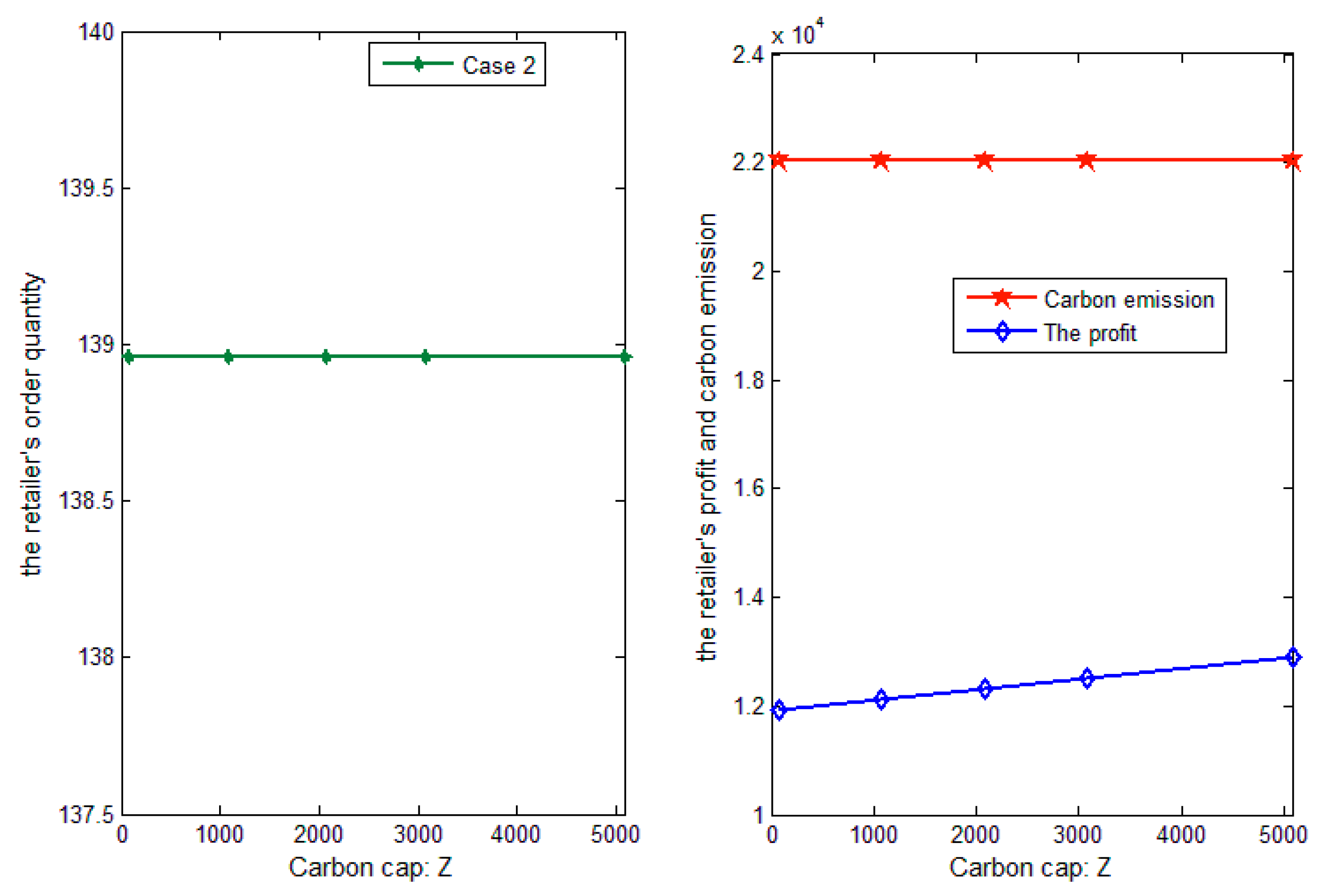
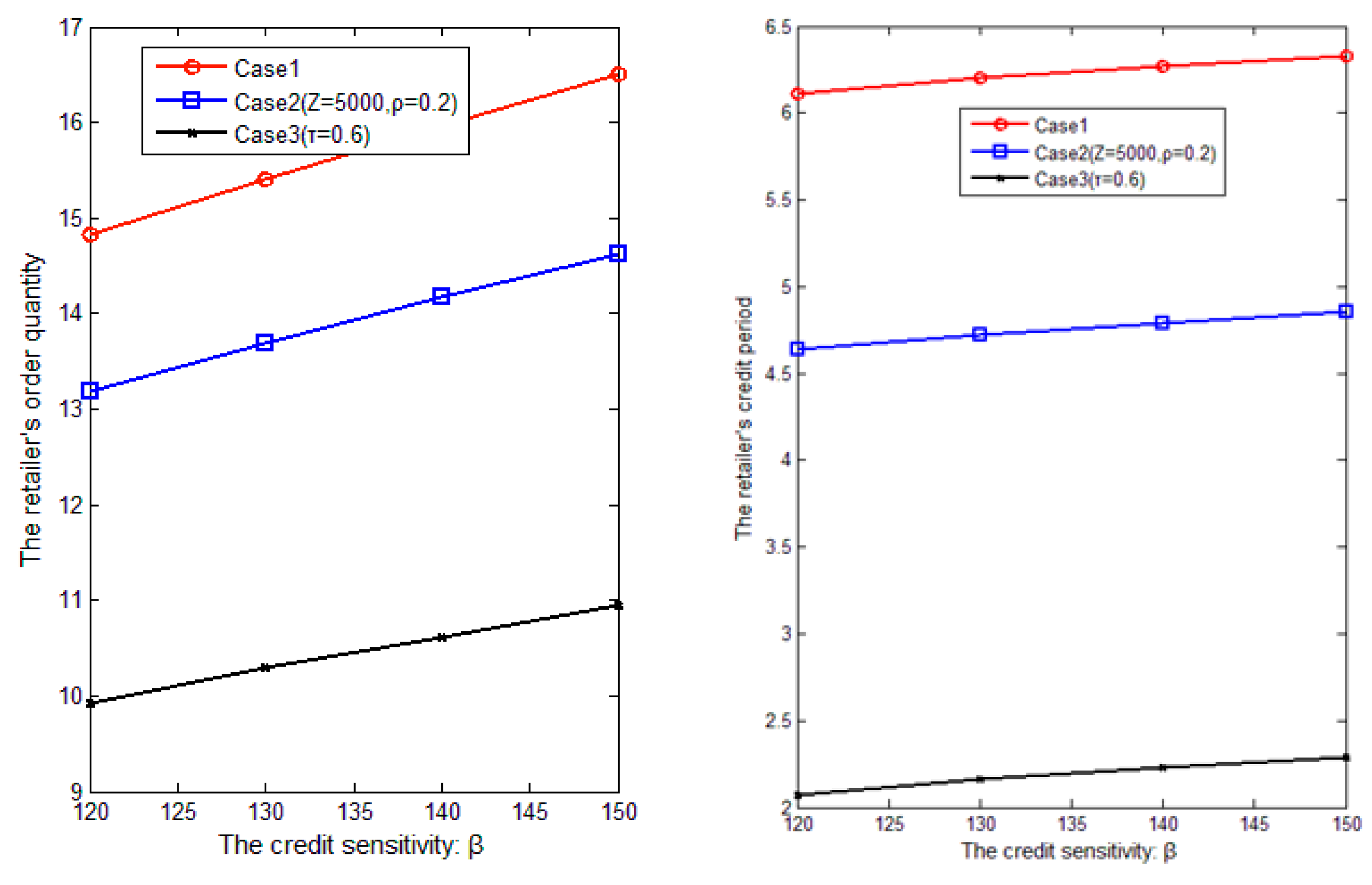
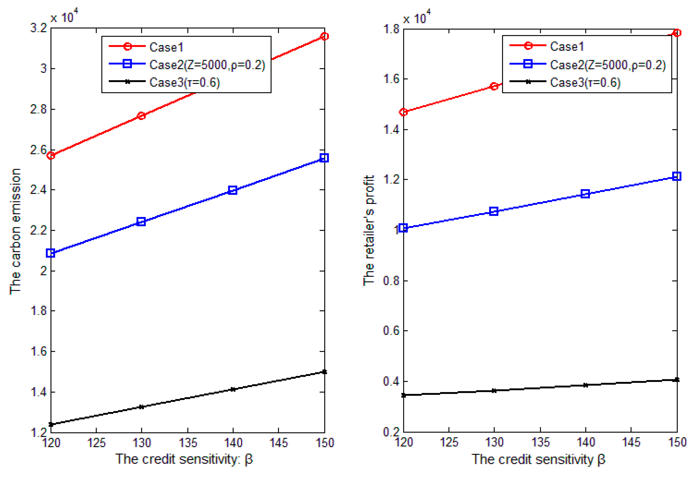
7.1.2. Endogenous Credit Period

The influence of parameters on the optimal order quantity, credit period, and carbon emissions of retailers is studied in the endogenous credit period. The values of the parameters with optimal solution values meet the conditions of Theorems 1–6. Hence, the profit functions Π 1 ( n , Q ) ,   Π 2 ( n , Q ) ,  and  Π 3 ( n , Q ) are concave with n and Q. The profit functions Π 1 ( n , Q ) ,   Π 2 ( n , Q ) ,  and  Π 3 ( n , Q ) with n  and Q are drawn using Matlab 7.0. Therefore, the global optimal solutions of the order quantity and credit period can be obtained: Q 1 * = 16.51 , Q 2 * =   14.62 , Q 3 * = 10.95 , n 1 * = 6.33 , n 2 * =   4.86 , and   n 3 * = 2.29 , respectively.
Similar to that in the exogenous credit period with the increase of carbon cap Z, the optimal credit period and order quantity are unchanged, but the profit increases. Therefore, effects of the following parameters on the decisions are emphasized.
Figure 8 shows that the optimal credit period, order quantity, carbon emissions, and profit of the retailer all increase with the increase of parameter β . When the consumers’ credit sensitivity is increasing, the retailer will increase the credit period to induce more market demand. Hence, the retailer offers a longer credit period for the consumers with higher credit sensitivity in order to increase market demand and profit. In comparison, the retailer offers a shorter credit period to consumers with enough money and who are not sensitive to a credit period to lessen the opportunity cost of the accounts receivable. The effect of parameter β on the carbon emissions in the endogenous credit period is more than that in the exogenous credit period (Figure 3).
Figure 9 shows that the optimal credit period, optimal order quantity, and profit of the retailer decrease as a result of the increase of impact factor δ of carbon emissions to the demand. The retailer shortens the trade credit period when the environmental sensitivity of the consumer increases. Under the parameters conditions, the credit period is decreasing with the consumers’ environmental sensitivity. It is counter intuitive since we usually think the retailer will relax the credit to induce more market demand when faced with the higher consumers’ environmental sensitivity. However, as the consumers’ environmental sensitivity increasing, the relative sensitivity of credit period respected to the environmental sensitivity decreases, which results in less effect on the demand. Moreover, because the higher credit period will induce more default risk cost and opportunity cost. Hence, after trading off the revenue and cost of the higher credit period, the retailer will tighten the credit period. The effect of parameter δ on the carbon emissions and the order quantity in the endogenous credit period is more than that in the exogenous credit period (Figure 4). This means that the consumers’ environmental sensitivity should be a great concern when the retailer has the power to decide the credit policies.
Figure 10 shows that the optimal credit period, order quantity, and profit decrease of the retailer decrease with the increase of the parameter ρ . Moreover, the optimal credit period, order quantity, and profit decrease under carbon tax regulation and with the increase of the parameter τ . As the carbon trade price or carbon taxes increasing, it will result in higher carbon emission cost. Hence, the retailer will provide the shorter credit period, which will accelerate the cash flow and reduce the default risk cost and the opportunity cost. The cap under the carbon cap-and-trade regulation has no effect on credit period decisions. However, carbon trade price and carbon taxes have a negative effect on the credit period from the retailer. When the government continues its high carbon price regulation, the retailer tightens the credit period by trading off the carbon emissions cost and the revenue of the longer credit period to lessen the opportunity cost of the accounts receivable. The effect of parameter ρ on the carbon emissions in the endogenous credit period is more than that in the exogenous credit period (Figure 5). The carbon regulations improve their effect on carbon emissions reduction when the retailer has the power to decide on credit policies.
Figure 8. Impacts of β on the decisions, profit, and carbon emissions of the retailer.
Sustainability 07 15818 g008aSustainability 07 15818 g008b
Figure 9. Impacts of δ on the decisions, profit, and carbon emissions of the retailer.
Sustainability 07 15818 g009
Figure 10. Impacts of carbon trade price or carbon taxes on the decisions, profit, and carbon emissions of the retailer.
Sustainability 07 15818 g010

7.2. Sensitivity Analysis of Multi Parameters: Monte Carlo Approach

Monte Carlo simulation is adopted to discuss how the variability of a system can propagate to the final results. The simulation method can be used in the following steps: (1) the mathematical model is defined; (2) a set of random inputs is generated; and (3) the process output is simulated and analyzed. Sensitivity analysis evaluates the effects of each key parameter on the system yields. The sensitivity analysis is executed by changing a single key model parameter to ±10% and ±20% with the original values. The influences of each parameter on the system yields are evaluated by calculating the value of response (S) using [55]
S = V 2 V 1 V 1  
where V2 is the yield for the single parameter mean value that is changed and V1 is the yield with all the parameter mean values that are unchanged.
The model has more than ten parameters, many of which have been discussed in literature. Hence, five key parameters in the model are chosen for the Monte Carlo simulation. The basic values are the same as in Section 7.1, except that β N ( 200 , 50 ) , δ N ( 0.03 , 0.0001 ) , k N ( 0.05 , 0.0001 ) Z N ( 5000 , 100 ) , and ρ N ( 0.2 , 0.01 ) . Based on the random values and after 2000 times simulation, the mean values for optimal solutions in Case 2 of the cap-and-trade regulation with endogenous credit period can be obtained as follows: n ¯ = 5.473 , Q ¯ = 18.215 , π ¯ = 20714 , and C O 2 ¯ = 26,680 . Similar to Case 2, that values are easy to obtain in Case 1 with Z = 0 and ρ = 0 and Case 3 with Z = 0 .
Equation (11) indicates that the sensitivity analysis of the key parameters can be performed (Table 2, Table 3, Table 4 and Table 5). Table 2 shows that the default risk has the highest response value for the optimal credit period, followed by carbon trade price. Table 3 presents that the carbon cap has the lowest response value for the optimal order quantity, followed by the carbon trade price. Table 4 and Table 5 illustrate that customers’ credit sensitivity has the greatest effect on carbon emission and enterprise profit among the key parameters when parameter change is positive. However, the customers’ carbon emission environmental sensitivity has the greatest influence on carbon emission and enterprise profit when parameter change is negative.
Table 2. Impact of key parameters on optimal credit period.
n Adjusted Value
10%−10%20%−20%
β −0.01250.0147−0.02280.0339
δ 0.0018−0.00120.0026−0.0023
k 0.0420−0.19910.1569−0.4637
Z−1.23 × 10−92.96 × 10−9−9.10 × 10−105.87 × 10⁻¹⁰
ρ 0.0115−0.05350.0388−0.0732
Table 3. Impact of key parameters on order quantity.
Q Adjusted Value
10%−10%20%−20%
β −0.04290.0488−0.09290.1023
δ 0.0274−0.07660.0667−0.1423
k 0.0306−0.06570.0800−0.1545
Z2.71 × 10−81.37 × 10⁻⁸−8.61 × 10−83.81 × 10−8
ρ 0.0101−0.01920.0226−0.0284
Table 4. Impacts of parameters on carbon emission.
C Q 2 Adjusted Value
10%−10%20%−20%
β −0.09610.0921−0.18960.1887
δ 0.0027−0.21190.0898−0.4215
k 0.0418−0.15690.1362−0.3741
Z−8.58 × 10−102.44 × 10⁻⁹−8.16 × 10−104.95 × 10⁻⁹
ρ 0.0122−0.04120. 0347−0.0579
Table 5. Impacts of parameters on the optimal profit of the retailer.
π Adjusted Value
10%−10%20%−20%
β −0.08670.0831−0.17180.1693
δ 0.0045−0.21750.0894−0.4436
k 0.0406−0.13980.1250−0.3389
Z−0.00670.0066−0.01290.0131
ρ 0.0082−0.07110.0412−0.0974

8. Conclusions

Under the constraints of carbon emissions regulations, this paper investigated the trade-off between the revenue and cost of trade credit while considering the environmental sensitivity of consumers. The study aimed to help enterprises make reasonable credit and operational decisions and improve the performance and sustainability of the supply chain operation. First, the decision models are analyzed under three cases: without regulation, carbon cap-and-trade regulation, and carbon tax regulation. The optimal solutions of the retailer in these three cases with exogenous and endogenous credit periods are then discussed. Finally, a couple of numerical analyses are given to obtain some conclusions.
The retailer shortens the trade credit period as the effect of the environmental sensitivity of consumers is enhanced. The credit risk induces high carbon emissions and less profit, which are bad for society’s welfare and the profit of the firm. The retailer offers longer credit period for consumers with high credit sensitivity to induce market demand and increase profit. The cap under the carbon cap-and-trade regulation has no effect on credit period decisions, whereas carbon trade price and carbon taxes have a negative effect on the credit period from the retailer. The retailer under carbon cap-and-trade regulation has more reasons to obey the regulations than that under carbon tax regulation when the carbon trade price equals carbon taxes. Moreover, carbon cap lessens the effect of carbon price on profit. Carbon regulations have a better effect on carbon emissions reduction when the retailer has the power to decide the credit policies.
Based on the Monte Carlo simulation, the default risk has the highest response value for the optimal credit period, followed by carbon trade price. Meanwhile, carbon cap has the lowest response value for the optimal order quantity, followed by the carbon trade price. In terms of carbon emission and the enterprise profit, the customers’ credit sensitivity has the greatest influence when the parameters change positively. However, the customers’ carbon emission environmental sensitivity has the greatest effect when the parameters change negatively.
This paper has some interesting extensions. Carbon emissions reduction technology has been investigated in the literature. Therefore, emissions reduction technology investments can be included in the future extended model. Moreover, coordination is the core focus of the supply chain; hence, a coordination mechanism to improve the supply chain performance with the trade credit and carbon emissions regulation can be discussed in future research.

Acknowledgments

This paper is funded by The National Natural Science Foundation of China 71302115, 71502123,), Education Ministry of Humanities and Social Science Research (13YJC630121), Young Scholar Program of Tianjin University of Finance and Economics, and Tianjin University Innovation Team Training Program (TD12-5051).

Author Contributions

Juanjuan Qin contributed to the design, conducted this research as well as wrote and revised the whole paper. Xiaojian Bai jointly conducted the research, solved some models, and was responsible for performing the numerical studies. Liangjie Xia contributed in the research and discussion and gave valuable suggestions.

Conflict of Interests

The authors declare no conflict of interest.

References

  1. IPCC. Climate Change 2007: The Physical Science Basis, 2007. Available online: http://www.slvwd.com/agendas/Full/2007/06-07-07/Item%2010b.pdf (accessed on 4 December 2015).
  2. Toptal, A.; Özlü, H.; Konur, D. Joint decisions on inventory replenishment and emission reduction investment under different emission regulations. Int. J. Prod. Res. 2014, 52, 243–269. [Google Scholar] [CrossRef] [Green Version]
  3. He, P.; Zhang, W.; Xu, X. Production lot-sizing and carbon emissions under cap-and-trade and carbon tax regulations. J. Clean. Prod. 2015, 103, 241–248. [Google Scholar] [CrossRef]
  4. Benjaafar, S.; Li, Y.; Daskin, M. Carbon footprint and the management of supply chains: Insights from simple models. IEEE Trans. Autom. Sci. Eng. 2013, 10, 99–116. [Google Scholar] [CrossRef]
  5. Avi-Yonah, R.S.; Uhlmann, D.M. Combating Global Climate Change: Why a Carbon Tax is a Better Response to Global Warming than Cap and Trade, 2009. Available online: http://papers.ssrn.com/sol3/papers.cfm?abstract_id=1333673 (accessed on 4 December 2015).
  6. Cholette, S.; Venkat, K. The energy and carbon intensity of wine distribution: A study of logistical options for delivering wine to consumers. J. Clean. Prod. 2009, 17, 1401–1413. [Google Scholar] [CrossRef]
  7. Stock, J.R.; Boyer, S.L.; Harmon, T. Research opportunities in supply chain management. J. Acad. Mark. Sci. 2010, 38, 32–41. [Google Scholar] [CrossRef]
  8. Petersen, M.A.; Rajan, R.G. Trade credit: Theories and evidence. Rev. Financ. Stud. 1997, 10, 661–691. [Google Scholar] [CrossRef]
  9. Williams, F. World bank urged to lift trade credit finance. Financial Times, 11 November 2008. [Google Scholar]
  10. Yang, S.A.; Birge, J.R. How Inventory is (Should be) Financed: Trade Credit in Supply Chains with Demand Uncertainty and Costs of Financial Distress, 2013. Available online: http://dx.doi.org/10.2139/ssrn.1734682 (accessed on 4 December 2015).
  11. Miller, R. Does everyone have a price. Marketing 1997, 24, 30–33. [Google Scholar]
  12. Hovelaque, V.; Bironneau, L. The carbon-constrained EOQ model with carbon emission dependent demand. Int. J. Prod. Econ. 2015, 164, 285–291. [Google Scholar] [CrossRef]
  13. Upham, P.; Dendler, L.; Bleda, M. Carbon labelling of grocery products: public perceptions and potential emissions reductions. J. Clean. Prod. 2011, 19, 348–355. [Google Scholar] [CrossRef]
  14. Bemporad, R.; Baranowski, M. Conscious Consumers are Changing the Rules of Marketing. Are You Ready? 2007. Available online: https://www.fmi.org/docs/sustainability/BBMG_Conscious_Consumer_White_Paper.pdf (accessed on 4 December 2015).
  15. Pontin, J. Q&A with Bill Gates. Available online: http://www.technologyreview.com/qa/420342/qa-bill-gates/ (accessed on 4 December 2015).
  16. Covert, R.P.; Philip, G.C. An EOQ model for items with Weibull distribution deterioration. AIIE Trans. 1973, 5, 323–326. [Google Scholar] [CrossRef]
  17. Huang, Y.F. Optimal retailer’s ordering policies in the EOQ model under trade credit financing. J. Op. Res. Soc. 2003, 54, 1011–1015. [Google Scholar] [CrossRef]
  18. Goyal, S.K. Economic order quantity under conditions of permissible delay in payments. J. Op. Res. Soc. 1985, 36, 335–338. [Google Scholar] [CrossRef]
  19. Chu, P.; Chang, K.H.; Lan, S.P. Economic order quantity of deteriorating items under permissible delay in payments. Comput. Op. Res. 1998, 25, 817–824. [Google Scholar] [CrossRef]
  20. Jamal, A.M.; Sarker, B.R.; Wang, S. An ordering policy for deteriorating items with allowable shortage and permissible delay in payment. J. Op. Res. Soc. 1997, 48, 826–833. [Google Scholar] [CrossRef]
  21. Teng, J.T.; Chang, C.T.; Chern, M.S. Vendor–buyer inventory models with trade credit financing under both non-cooperative and integrated environments. Int. J. Syst. Sci. 2012, 43, 2050–2061. [Google Scholar] [CrossRef]
  22. Liao, J.J.; Huang, K.N.; Chung, K.J. Lot-sizing decisions for deteriorating items with two warehouses under an order-size-dependent trade credit. Int. J. Prod. Econ. 2012, 137, 102–115. [Google Scholar] [CrossRef]
  23. Tsao, Y.C.; Chen, T.H.; Zhang, Q.H. Effects of maintenance policy on an imperfect production system under trade credit. Int. J. Prod. Res. 2013, 51, 1549–1562. [Google Scholar]
  24. Cárdenas-Barrón, L.E. The economic production quantity (EPQ) with shortage derived algebraically. Int. J. Prod. Econ. 2001, 70, 289–292. [Google Scholar] [CrossRef]
  25. Chung, K.J.; Huang, Y.F. The optimal cycle time for EPQ inventory model under permissible delay in payments. Int. J. Prod. Econ. 2003, 84, 307–318. [Google Scholar] [CrossRef]
  26. Ho, C. H.; Ouyang, L.Y.; Su, C.H. Optimal pricing, shipment and payment policy for an integrated supplier-buyer inventory model with two-part trade credit. Eur. J. Op. Res. 2008, 187, 496–510. [Google Scholar] [CrossRef]
  27. Chung, K.J.; Liao, J.J. The simplified solution algorithm for an integrated supplier buyer inventory model with two-part trade credit in a supply chain system. Eur. J. Op. Res. 2011, 213, 156–165. [Google Scholar] [CrossRef]
  28. Sarkar, B. An EOQ model with delay in payments and time varying deterioration rate. Math. Comput. Model. 2012, 55, 367–377. [Google Scholar] [CrossRef]
  29. Min, J.; Zhou, Y.W.; Liu, G.Q. An EPQ model for deteriorating items with inventory-level-dependent demand and permissible delay in payments. Int. J. Syst. Sci. 2012, 43, 1039–1053. [Google Scholar] [CrossRef]
  30. Soni, N.H. Optimal replenishment policies for non-instantaneous deteriorating items with price and stock sensitive demand under permissible delay in payment. Int. J. Prod. Econ. 2013, 146, 259–268. [Google Scholar] [CrossRef]
  31. Su, C.H.; Ouyang, L.Y.; Ho, C.H.; Chang, C.T. Retailer’s inventory policy and supplier’s delivery policy under two-level trade credit strategy. Asia. Pac. J. Op. Res. 2007, 24, 613–630. [Google Scholar] [CrossRef]
  32. Jaggi, C.K.; Goyal, S.K.; Goel, S.K. Retailer’s optimal replenishment decisions with credit-linked demand under permissible delay in payments. Eur. J. Op. Res. 2008, 190, 130–135. [Google Scholar] [CrossRef]
  33. Jaggi, C.K.; Kapur, P.K.; Goyal, S.K.; Goel, S.K. Optimal replenishment and credit policy in EOQ model under two-levels of trade credit policy when demand is influenced by credit period. Int. J. Syst. Assur. Eng. Manag. 2012, 3, 352–359. [Google Scholar] [CrossRef]
  34. Thangam, A.; Uthayakumar, R. Two-echelon trade credit financing for perishable items in a supply chain when demand depends on both selling price and credit period. Comput. Ind. Eng. 2009, 57, 773–786. [Google Scholar] [CrossRef]
  35. Giri, B.C.; Maiti, T. Supply chain model with price-and trade credit-sensitive demand under two-level permissible delay in payments. Int. J. Syst. Sci. 2013, 44, 937–948. [Google Scholar] [CrossRef]
  36. Lou, K.R.; Wang, W.C. Optimal trade credit and order quantity when trade credit impacts on both demand rate and default risk. J. Oper. Res. Soc. 2012, 64, 1551–1556. [Google Scholar] [CrossRef]
  37. Wu, J.; Chan, Y.L. Lot-sizing policies for deteriorating items with expiration dates and partial trade credit to credit-risk customers. Int. J. Prod. Econ. 2014, 155, 292–301. [Google Scholar] [CrossRef]
  38. Wu, J.; Ouyang, L.Y.; Barron, L.; Goyal, S. Optimal credit period and lot size for deteriorating items with expiration dates under two level trade credit financing. Eur. J. Op. Res. 2014, 237, 898–908. [Google Scholar] [CrossRef]
  39. Zhang, Q.; Dong, M.; Luo, J.; Segerstedt, A. Supply chain coordination with trade credit and quantity discount incorporating default risk. Int. J. Prod. Econ. 2014, 153, 352–360. [Google Scholar] [CrossRef]
  40. Liu, Z.L.; Anderson, T.D.; Cruz, J.M. Consumer environmental awareness and competition in two-stage supply chains. Eur. J. Op. Res. 2012, 218, 602–613. [Google Scholar] [CrossRef]
  41. Glock, C.H.; Jaber, M.Y.; Searcy, C. Sustainability strategies in an EPQ model with price-and quality-sensitive demand. Int. J. Logist. Manag. 2012, 23, 340–359. [Google Scholar] [CrossRef]
  42. Swami, S.; Shah, J. Channel coordination in green supply chain management. J. Op. Res. Soc. 2012, 64, 336–351. [Google Scholar] [CrossRef]
  43. Nouira, I.; Frein, Y.; Hadj-Alouane, A.B. Optimization of manufacturing systems under environmental considerations for a greenness-dependent demand. Int. J. Prod. Econ. 2014, 150, 188–198. [Google Scholar] [CrossRef]
  44. Zhang, L.; Wang, J.; You, J. Consumer environmental awareness and channel coordination with two substitutable products. Eur. J. Op. Res. 2015, 241, 63–73. [Google Scholar]
  45. Du, S.; Zhu, J.; Jiao, H.; Ye, W. Game-theoretical analysis for supply chain with consumer preference to low carbon. Int. J. Prod. Res. 2015, 53, 3753–3768. [Google Scholar] [CrossRef]
  46. He, L.; Zhao, D.; Xia, L. Game Theoretic Analysis of Carbon Emission Abatement in Fashion Supply Chains Considering Vertical Incentives and Channel Structures. Sustainability 2015, 7, 4280–4309. [Google Scholar]
  47. Hua, G.; Cheng, T.C.E.; Wang, S. Managing carbon footprints in inventory management. Int. J. Prod. Econ. 2011, 132, 178–185. [Google Scholar] [CrossRef]
  48. Hua, G.; Qiao, H.; Jian, L. Optimal order lot sizing and pricing with carbon trade. 2011. Available online: http://papers.ssrn.com/sol3/papers.cfm?abstract_id=1796507 (accessed on 4 December 2015).
  49. Song, J.; Leng, M. Analysis of the single-period problem under carbon emissions policies. In Handbook of Newsvendor Problems; Springer: New York, NY, USA, 2012; pp. 297–313. [Google Scholar]
  50. Arslan, M.; Metin, T. EOQ revisited with sustainability considerations. Found. Comput. Decis. Sci. 2013, 38, 223–249. [Google Scholar]
  51. Chen, X.; Benjaafar, S.; Elomri, A. The carbon-constrained EOQ. Op. Res. Lett. 2013, 41, 172–179. [Google Scholar] [CrossRef]
  52. Dye, C.Y.; Yang, C.T. Sustainable trade credit and replenishment decisions with credit-linked demand under carbon emission constraints. Eur. J. Op. Res. 2015, 244, 187–200. [Google Scholar] [CrossRef]
  53. Teng, J.T.; Lou, K.R.; Wang, L. Optimal trade credit and lot size policies in economic production quantity models with learning curve production costs. Int. J. Prod. Econ. 2014, 155, 318–323. [Google Scholar] [CrossRef]
  54. Zanoni, S.; Mazzoldi, L.; Zavanella, L.E.; Jaber, M.Y. A joint economic lot size model with price and environmentally sensitive demand. Prod. Manuf. Res. 2014, 2, 341–354. [Google Scholar]
  55. Samsudin, M.D.M.; Don, M.M. Assessment of bioethanol yield by S. cerevisiae grown on oil palm residues: Monte Carlo simulation and sensitivity analysis. Bioresour. Technol. 2015, 175, 417–423. [Google Scholar] [CrossRef] [PubMed]

