Integrating a Spatially Explicit Tradeoff Analysis for Sustainable Land Use Optimal Allocation

Abstract

To achieve agricultural sustainability, basic land planning would allocate more areas for specific land uses with high ecosystem service values. However, this has always failed because of its low economic interest. Paying farmers would be effective for its implementation. To overcome previous studies’ limitation in spatial display, we developed a novel approach with a spatially explicit land use plan under payment policy. It integrates the tradeoff analysis into a traditional land use optimal allocation system. The land allocation system generates an origin land use scenario. Our method analyzes farmers’ tradeoffs in changing crops by adopting payment policy. Finally, the origin land use map is reallocated. The newly reclaimed region of Yili, China is studied as a representative area. Our tool established a tradeoff curve indicating the adoption proportion of farmers changing other land use types to clover, which is a specific crop with high ecosystem service values, at different payment prices. Areas adopting the payment policy were identified, and corresponding spatial distribution maps of land use re-allocation were generated for the tradeoff curve. Sensitivity analysis validated the robustness of our model. Results demonstrated that our method can provide more spatial and economic information for sustainable land use planning.

1. Introduction

Increases in agricultural output from limited arable land are essential, driven by population growth and increasing food demand [1,2]. Yet, agricultural production activities will threaten the environmental integrity of local landscapes and the global ecosystem. There is an urgent need to reduce the adverse impact of the agricultural system on the environment [2] and to achieve agricultural sustainability [1,3]. A rational and effective land use optimal allocation system, as a type of land resource allocation planning, is important to integrate economic development, environmental protection, efficient resource use, and social equity. It will ensure production of sufficient food and fiber at an acceptable environmental cost [1,3,4].

There are many approaches to optimal land use allocation, which includes swarm optimization [5], simulated annealing [6], genetic algorithms [7,8], and goal programming [9]. These methods integrate social, economic, and environmental benefits in model criteria and objectives. Ecological and environmental impacts are included in the programming model constraints or the target equations, which design sustainable land allocation planning with more areas for specific land uses with high ecosystem service values [7,8,9]. However, this cannot reflect farmers’ and other stakeholders’ economic benefits and their potential support for land use planning to protect the environment. Farmers would decide the land use based upon the expected net return of the crops. Therefore, the land use allocation program takes on a strongly idealistic character, which is a mandatory planning set for the government but is not easily adopted by farmers. To increase the supply of ecosystem services and achieve agricultural sustainability, the government or public sector implement the payment policy to compensate farmers to turn to land uses with low economic value but high ecological benefits [1,3,4].

With the payment policy, farmers make a tradeoff between the origin land use type and the specific type with payments attached and determine whether to change the land use. Also, the government makes a tradeoff between the ecosystem service benefits and environmental compensation costs. An ex ante analysis of quantifying these tradeoffs is critical in designing sustainable land planning [10,11]. A tradeoff analysis model between environmental and economic indicators was developed to provide policy decision makers with essential information about agricultural production systems [11,12,13]. A tradeoff curve and corresponding spatial variation among ecosystem services and payments were simulated. These tools will help achieve high utilization of agricultural land resources and sustainable development.

The tradeoff model [11,12,13] requires a large quantity of high quality data for the physical and economic models. However, high-resolution biophysical and economic data on the geographic coverage are exceptional, but provide limited economic information. In most cases, site-specific economic data are only available from special-purpose farm surveys, and the time and resources required to undertake special-purpose surveys preclude their use for most policy analysis. Moreover, this is a challenge in developing countries. The development and application of a quick and low-cost method for ex ante evaluation of land planning are needed [14,15,16,17,18]. A tradeoff analysis-minimum data (TOA-MD) approach is proposed to provide timely and accurate information to support policy decision making [14,15,16,17,18]. Compared with the origin tradeoff model, the TOA-MD provides a tradeoff curve with similar accuracies [18]. However, it cannot reflect the spatial variability of the output, which can display where would adopt the payment policy and where would stay stable at different payments. Especially in land use planning, the variation in tradeoff outcomes may be more interesting than the aggregated results [12]. Spatial information on land use planning under the payment policy would be more effective for supporting decision making.

The objective of this paper is to develop a spatially explicit and low-cost approach for sustainable land use planning under the payment policy. Our strategy is to integrate the tradeoff analysis with the traditional land use optimal allocation model at a spatial dimension. We intend to link these two by calculating the spatial opportunity costs of changing crops under the payment policy and simulating farmers’ tradeoff analysis on land uses. Areas where farmers adopt the payment policy and change land uses after a tradeoff analysis on return of different land uses can be simulated. Then we can reallocate the above area to new land use for the spatial distribution of origin land use planning using payments for ecosystem services.

2. Materials and Methods

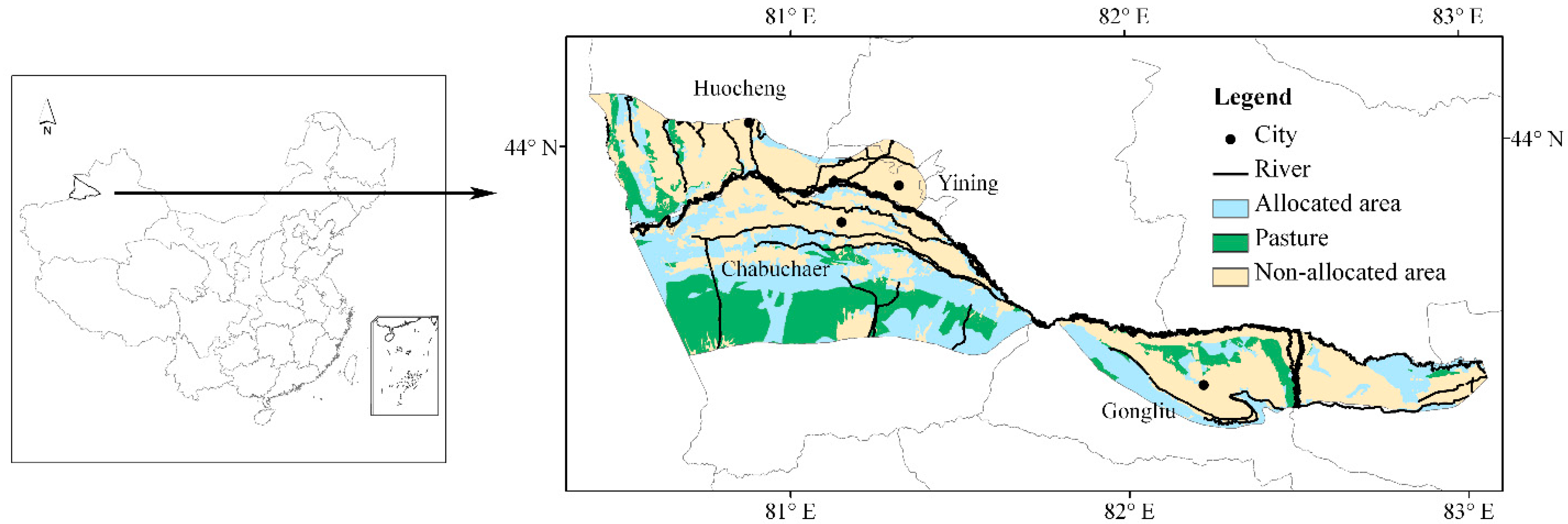
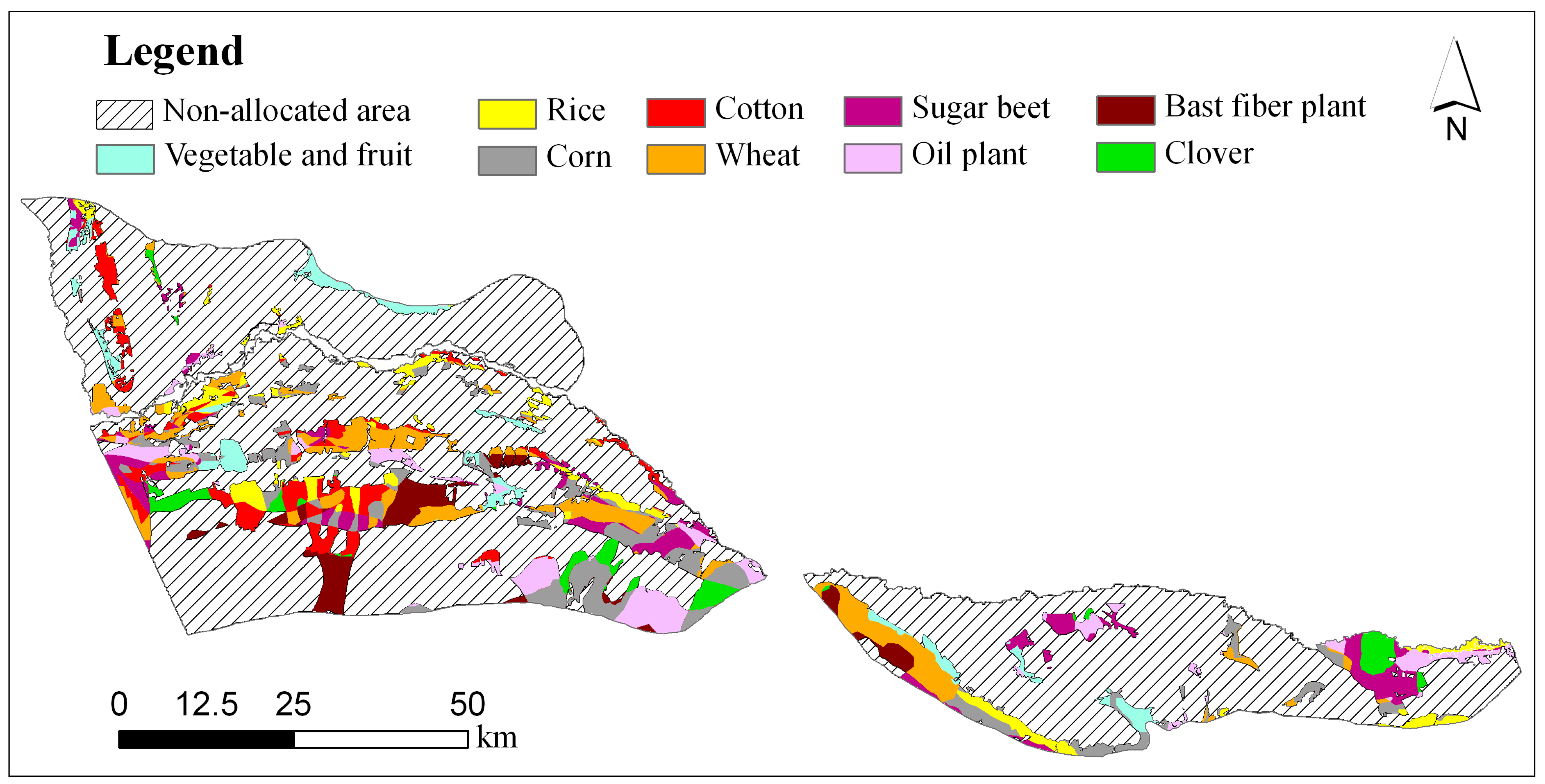
2.1. Study Area

The newly reclaimed region is located in the valley of Yili, Xinjiang and lies roughly between 80°22'14"N–83°3'54"N and 43°22'37"N–44°8'22"N (Figure 1). It is one of seven important land resource development regions established by the Ministry of Land and Resources of the People’s Republic of China. The region covers an area of approximately 5000 km², with elevations ranging from 661 m to 1572 m. It lies within the temperate-continental, semi-arid climate zone, with a mean annual temperature of 8–9 °C, a mean annual precipitation of 200–500 mm, and a mean annual evaporation of 1200–1900 mm, with water resources that are the richest in Xinjiang. It should be noted that the land use optimal allocation area should exclude conservation areas, construction lands, and mature agricultural lands. For agricultural allocation especially, pastures are excluded. Then the excluded areas were noted as “non-allocated areas” in this study.

Figure 1. Location of the newly reclaimed region of Yili.

Figure 1. Location of the newly reclaimed region of Yili.

Most of the region has a high ecological sensitivity, with a relatively large slope area, a thin sandy soil layer, and low soil fertility. Improper land use choice and allocation is likely to cause erosion, land desertification, and soil salinization [19]. Rational land use planning in the region is essential to prevent degradation, and the land optimal allocation system in the newly reclaimed region is anticipated to address conflicts between economic benefit and ecological protection.

2.2. Methods and Data Description

The flowchart in Figure 2 displays a series of basic steps for implementing our tool. Application of this approach, based on a raster, is mainly in three stages: land use spatial allocation, opportunity costs calculation, and tradeoff analysis. The agricultural land use optimal allocation (ALUOA) system [20] was applied in the first stage. The spatial opportunity costs calculation is the intermediate stage that integrates the tradeoff analysis with the ALUOA system. Then it determines the final land use spatial reallocation based on the payment policy. We designated the improved tool as the “ALUOA-TOA” system.

Figure 2. Flowchart of the integration of trade analysis and the land use optimal allocation system.

Figure 2. Flowchart of the integration of trade analysis and the land use optimal allocation system.

Firstly, our method uses the ALUOA system to generate an origin land use allocation map, which aims to maximize the economic income and would be realistic for farmers’ adoption without any payments. Secondly, it simulates opportunity costs of different land uses under the payment policy by calculating the potential crop yields and net returns. Different payment prices result in different opportunity costs for farmers’ crop selection and change. Finally, our method simulates the tradeoff of famers and the government. With the economic incentive from payments, farmers make the tradeoff on economic incomes of different crops and decide whether to adopt the payment policy. Meanwhile, the government would evaluate a reasonable payment price, which is a tradeoff on the environmental compensation and ecosystem service benefit. Then areas of crop change were identified and the original land uses were reallocated in a spatial display.

The details of our framework are as follows, with a case study. All data were processed and converted to pixels with 25-m resolution in ArcGIS 9.3 (ESRI Inc., Redlands, CA, USA). The 25-m pixel is seen as the analysis unit reflecting the farmers’ behavior.

2.2.1. Land Use Spatial Allocation

The ALUOA system was developed by our study team and applied in the newly reclaimed region. It consists of three steps: land suitability evaluation (LSE), land use area optimization, and land use spatial allocation [20]. Interested readers can find content details in paper [20]. The LSE assesses the degree of satisfaction of the crop requirement by using a weighted linear method for summing up different evaluation criteria, which include soil qualities, terrain factors, water supply conditions, climatic data, and socially locational factors (Table 1). In this study, wheat, corn, rice, cotton, sugar beets, oil plant, bast fiber plants, clover, vegetables, and fruit are crop types for planning purposes, according to the agricultural crop structure in the newly reclaimed region.

Table 1. Land suitability evaluation criteria, data source, and processing.

Criterion	Input dataset	Data source	Format	Processing
Soil texture	1:100,000 Soil type maps of Yili region	Institute of Geographical Sciences and Natural Resources Research	polygon	Format transformation
Soil depth	Soil sampling points	Fieldwork by the research team	point	Kriging interpolation
Soil organic matter	Soil sampling points	Fieldwork by the research team	point	Kriging interpolation
Sand dune waviness	1:50,000 Topographic maps; Land use map 2008	Institute of Geographical Sciences and Natural Resources Research; Data Center for Resources and Environmental Sciences, Chinese Academy of Sciences	raster	Selecting the sand distribution from the land use map and calculating the relative height from the DEM digitized from the topographic maps
Soil erosion	1:50,000 Topographic maps	Institute of Geographical Sciences and Natural Resources Research	raster	Calculating the gully density from the above DEM
Water supply and drainage	1:100,000 Land resource map of China	Institute of Geographical Sciences and Natural Resources Research	raster	Resampling
Salinity	1:100000 Soil type maps of Yili region; 1:1000000 Land resource map	Institute of Geographical Sciences and Natural Resources Research	raster	Format transformation
> 10 °C accumulated temperature	1:1000000 Accumulated temperature map of Yili region	Institute of Geographical Sciences and Natural Resources Research	raster	Format transformation
Nearest distance to towns	1:100000 Spatial map of towns in Yili region	Data Center for Resources and Environmental Sciences, Chinese Academy of Sciences	raster	Distance calculation
Nearest distance to roads	1:100000 Spatial map of roads in Yili region	Data Center for Resources and Environmental Sciences, Chinese Academy of Sciences	raster	Distance calculation

Table 1. Land suitability evaluation criteria, data source, and processing.

Criterion	Input dataset	Data source	Format	Processing
Soil texture	1:100,000 Soil type maps of Yili region	Institute of Geographical Sciences and Natural Resources Research	polygon	Format transformation
Soil depth	Soil sampling points	Fieldwork by the research team	point	Kriging interpolation
Soil organic matter	Soil sampling points	Fieldwork by the research team	point	Kriging interpolation
Sand dune waviness	1:50,000 Topographic maps; Land use map 2008	Institute of Geographical Sciences and Natural Resources Research; Data Center for Resources and Environmental Sciences, Chinese Academy of Sciences	raster	Selecting the sand distribution from the land use map and calculating the relative height from the DEM digitized from the topographic maps
Soil erosion	1:50,000 Topographic maps	Institute of Geographical Sciences and Natural Resources Research	raster	Calculating the gully density from the above DEM
Water supply and drainage	1:100,000 Land resource map of China	Institute of Geographical Sciences and Natural Resources Research	raster	Resampling
Salinity	1:100000 Soil type maps of Yili region; 1:1000000 Land resource map	Institute of Geographical Sciences and Natural Resources Research	raster	Format transformation
> 10 °C accumulated temperature	1:1000000 Accumulated temperature map of Yili region	Institute of Geographical Sciences and Natural Resources Research	raster	Format transformation
Nearest distance to towns	1:100000 Spatial map of towns in Yili region	Data Center for Resources and Environmental Sciences, Chinese Academy of Sciences	raster	Distance calculation
Nearest distance to roads	1:100000 Spatial map of roads in Yili region	Data Center for Resources and Environmental Sciences, Chinese Academy of Sciences	raster	Distance calculation

Three scenarios were developed based on the previous study [20]. The basic scenario was consistent with the agricultural structure of cereal, cash, and forage crops in the Yili region. Considering the common crop choices of four surrounding counties (Huocheng, Cabuchaer, Gongliu, and Xinyuan), cereal, cash, and forage crops account for 55.48%, 43.36%, and 1.15%, respectively, which represents a typical “cereal-cash” dualistic structure. Then we set the lower limit of percentages for cereal, cash, and forage crops as 50%, 30%, and 5%, respectively. Furthermore, wheat is a basic cereal food component in Yili; we set its proportion at not less than 20%. Based on crop farming trends and practices from the past 20 years, areas of rice and cotton will be expanded in the future. To curb the detrimental aspects of its development, we set the highest proportion of planting area for rice at not larger than 15%. With the above situations, we set these constraint conditions for the linear programming. The linear programming determined the optimal area of each land use type based on Equation (1) (constraint conditions) and Equation (2) (goal function) as follows:

$$\{\begin{array}{l}{x}_1+x_2+x_3\ge 0.5\\ x_4+x_5+x_6+x_7+x_8\ge 0.3\\ x_1\ge 0.2\\ x_3\le 0.15\\ x_4\le 0.15\\ x_9\ge 0.05\\ {\displaystyle \sum _{i=1}^9{{\displaystyle x}}_i=1}\\ x_1,x_2,x_3,\dots ,x_9\ge 0\end{array}$$

(1)

$$\begin{array}{l}I=\text{max}[(4240x_1+8029x_2+9717x_3+11849x_4+5195x_5\\ +6159x_6+4642x_7+26934x_8+3000x_9)\times A]\end{array}$$

(2)

where I means the total land resource economic income (unit: yuan); x₁, x₂, x₃, …, x₉ are the area proportions of wheat, corn, rice, cotton, sugar beets, oil plants, bast fiber plants, vegetables, fruits, and clover for the allocated area; and A is the area.

With the spatial distribution of LSE and the optimal area for each crop, the module allocates each land use type by a hierarchical optimal allocation method. Final land use spatial allocation maps are then generated. The basic scenario map was used in this study for the fundamental analysis (Figure 3). Two other land use scenarios are intended to adjust the agricultural structure and increase ecosystem service values to realize agricultural sustainability. This suggests that the reasonable agricultural structure in the Yili region should be adjusted at a higher proportion of livestock farming [21]. They were also designed with higher area proportions of clover than in the basic scenario.

Clover is a promising forage crop in the Yili region; it has higher economic value than traditional forage crops and an especially high ecosystem service in helping prevent land degradation [21]. Compared to other crops, which maintain the vegetable cover only in the growing season, clover maintains the vegetable cover in the whole year as a perennial crop. Continuous vegetable cover would effectively protect the soil, which could otherwise be easily eroded in the spring. In addition, it has a high ecosystem service value in sand fixation and soil conservation in the study area.

However, the economic benefit of clover is lower than many other crops’. The above two scenarios are intended to protect the environment and prevent land degradation—the policy goals of mandatory planning set by the government and experts—but are not easily adopted by farmers. To effectively implement the sustainable land use allocation planning, the government should provide farmers with payments to turn to clover, even though it has low economic benefits. Therefore, clover was chosen as the target crop of the payment policy for the tradeoff analysis in our study.

Figure 3. Spatial allocation map of the basic land use scenario.

Figure 3. Spatial allocation map of the basic land use scenario.

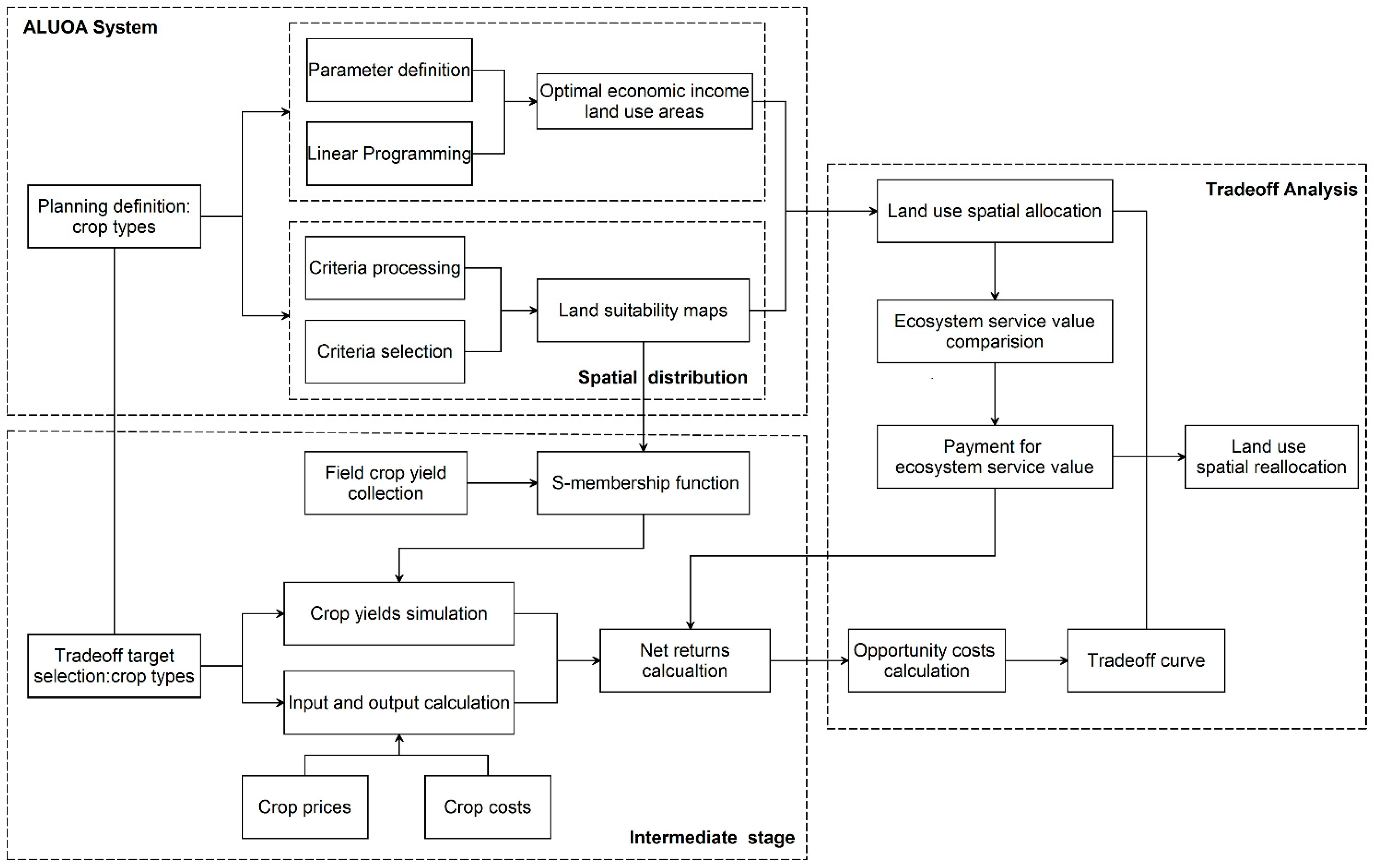
2.2.2. Conceptual Framework of Tradeoff Analysis

We integrated the tradeoff analysis with the ALUOA system to provide more information on land use planning. With payments for farmers provided by the government, the tradeoff analysis can evaluate how many lands would turn to clover at a specific payment price. Furthermore, our approach identified areas adopting the payment policy on the spatial display.

The tradeoff analysis in the ALUOA-TOA system was based on the TOA-MD model, with its basic assumptions [14,15,16,17,18] but some different settings. It assumes that farmers make land use and management decisions to maximize their perceived economic wellbeing. A farmer’s choice between two competing land uses (a and b) is determined by the opportunity cost [18] as follows:

$$\omega \left(r,s\right)=\nu \left(r,s,a\right)-\nu \left(r,s,b\right)$$

(3)

where ω is the opportunity cost; v is the excepted value on land uses, which is defined as the net return (yuan/ha) in our study; r is a vector of input and output prices for land uses; s indexes the site (and in this study s is a pixel); and a and b mean the land use at the pixel.

Alternately, it is assumed that practice b produces more ecosystem services than practice a, since the analysis here is based on the difference between the two practices. The parameter e(s) is interpreted as the expected ecosystem service values obtained from changing land use, not as the realized supply of ecosystem services. With the p_e as the ecosystem price (or payment price) for practice b, the income of practice b is v(r,s,b) + p_e·e(s), and the choice of farmers is assumed to be determined by Equation (4), as follows:

$$\omega (r,s,p_e)=\nu (r,s,a)-\nu (r,s,b)-p_e\cdot e(s)$$

(4)

If ω(r,s,p_e) ≥ 0, farmers adopt practice a; if ω(r,s,p_e) < 0, farmers adopt practice b. In particular, for the pixels where ω(r,s) < 0, farmers adopt practice b without any payments.

In previous studies, this can provide a summary proportion of farmers adopting the payment policy but cannot provide the spatial variability of farmers’ adoption [14,15,16,17,18]. It is unclear where practice b changes from practice a, a situation that will hamper decision making. Our strategy is to simulate the spatial distribution of opportunity costs for the tradeoff analysis. Then we can reallocate the basic land use scenario, changing practice a to practice b based on payments for farmers. From the spatial distribution of LSE scores, we can simulate the spatial distribution opportunity costs at each payment price in the tradeoff curve by applying series of crop yield simulations, input and output calculations, and opportunity costs calculations (Figure 2).

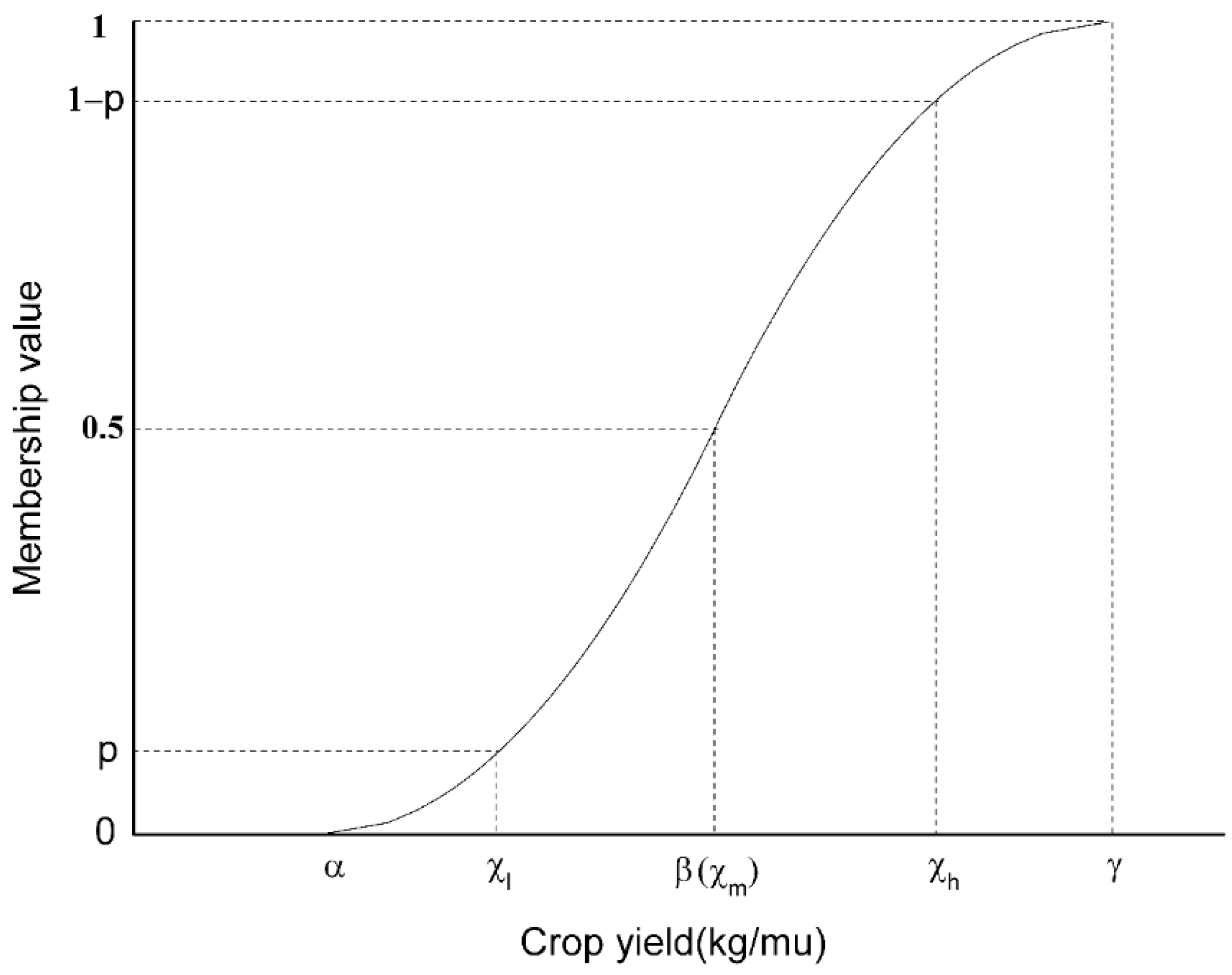
2.2.3. Crop Yield Simulation

LSE is the key in linking tradeoff analysis to the ALUOA system, which is a model for predicting potential land production [22,23]. The LSE is a prerequisite in achieving optimum utilization of the available land resources, while preserving highly suitable lands with high yields [24,25]. It collects and processes in mathematical equations climatic and other physical parameters that affect crop yields [26]. Thus it can also be used to predict the crop yield based on land suitability [23,27]. There have been numerous attempts to predict crop yields from data on land qualities using fuzzy S-membership functions, which are appropriate and robust for both quantitative and linguistic variables [28,29,30]. The membership function expresses the degree of an observed yield belonging to a certain LSE [28]. The S-membership function assume that a high LSE—a highly suitable condition for a certain crop growth—would determine a high crop yield but with a limit, and vice versa.

The input and management of the same crop were assumed to be the same in each pixel, which was accepted for an ex ante evaluation. Then potential crop yields are determined by the LSE. We used S-membership functions to estimate potential crop yields based on the available field crop yield data. The S-membership functions connect the crop yield to the specific land suitability score (Figure 4) [28,29,30], with the equation as follows:

$$S(\alpha ,\beta ,\gamma )=\{\begin{array}{ll}0,& x\in [-\infty ,\alpha ]\\ 2{[(x-\alpha )/(\gamma -\alpha )]}^2,& x\in [\alpha ,\beta ]\\ 1-2{[(x-\gamma )/(\gamma -\alpha )]}^2,& x\in [\beta ,\gamma ]\\ 1,& x\in [\gamma ,\infty ]\end{array}$$

(5)

where S means the membership value of crop yield to the land suitability score, x is the crop yield, α and γ are the lower and upper limits of crop yields, and β is (α + γ)/2. The α and γ are the ideal limits of crop yields at local conditions, which characterized soil qualities, terrain factors, water supply conditions, climatic data, and socially locational factors with the assumption of the same input and management. They belong to the worst and best LSE values, respectively, and the membership values are 0 and 1, respectively.

S should be calculated from the standardized land suitability scores using Equation (6):

$$S=(l-l_{min})/(l_{max}-l_{min})$$

(6)

where l is the land suitability score of a given crop at the pixel, and l_min and l_max are the lower and upper limits of land suitability scores in the whole study area.

The critical values (α and γ) of S-membership functions are usually difficult to determine and are always selected according to expert judgment and experience [31]. From the household survey and statistical data, we can collect the highest, mean, and lowest crop yields (defined as x_h, x_m, and x_l, where the x_m = (x_h + x_l)/2 = β). The actual yields are determined by various factors based on the ideal LSE condition; therefore, x_l and x_h would not be up to the lower and upper limits but are close to α and γ. We proposed a parameter p, which is the membership value of x_l and close to 0 (for example, the default setting of p is 0.1 in this case study). Then (1 – p) is the membership for x_h, which is close to 1. We can establish the following equation set:

$$\{\begin{array}{c}2{[(x_l-\text{α})/(\text{γ}-\text{α})]}^2=p\\ 1-2{[(x_h-\text{γ})/(\text{γ}-\text{α})]}^2=1-p\end{array}$$

(7)

Therefore, α and γ can be calculated from Equation (5). The crop yield can be calculated as follows:

$$x=\{\begin{array}{ll}\alpha +\left(\gamma -\alpha \right)\sqrt{S/2},& 0\le S<0.5\\ \gamma -(\gamma -\alpha )\sqrt{(1-S)/2},& 0.5\le S<1\end{array}$$

(8)

Figure 4. S-membership function to connect land use evaluation to crop yields.

Figure 4. S-membership function to connect land use evaluation to crop yields.

2.2.4. Ecosystem Service Value Estimation

The e(s) is interpreted as the expected ecosystem service values obtained from changing land use. However, ecosystem services include a considerable number of types [32] and we do not need to estimate all of them in our case study. Compared to other crops, clover has larger ecosystem service values in soil conservation, namely preventing land degradation in the Yili region. Therefore, we estimated the decrease of soil erosion as the supply of ecosystem service values from changing other crops to clover. The Universal Soil Loss Equation (USLE) is the most popular method used for soil erosion modeling and assessment [33] and was applied to quantify the amount of annual soil loss in the two situations described above. The equation of USLE is as follows:

$$A=R\times K\times L\times S\times C\times P$$

(9)

where A is the amount of average soil loss (ton·ha⁻¹·a⁻¹); R is the rainfall erosivity factor (MJ·mm·ha⁻¹·h⁻¹·a⁻¹); K is the soil erodibility factor (ton·ha·h·ha⁻¹·MJ⁻¹·mm⁻¹); L is the slope length factor; S is the slope factor; C is the vegetation cover factor; and P is the erosion control practice factor. Factors C and P are dimensionless.

With different crops at the same site, R, K, L, and S are the same and P is assumed to be the same for land use planning. Then e(s) (ton·ha⁻¹·a⁻¹) is represented as the change of C factor from changing crops to clover (ton·ha⁻¹·a⁻¹). It can be calculated by the following equation:

$$e(s)=\Delta A=R\times K\times L\times S\times P\times (C_a-C_b)$$

(10)

where C_b and C_a represent the vegetation cover factor of clover and other crops, respectively.

As we are lacking field data for C_b and C_a, we use the remote sensing estimation, which has been widely used in China, to calculate them [34]. The equations are as follows:

$$C=\{\begin{array}{ll}1& f=0\\ 0.6508-0.3436\lg f& 0<f\le 78.3\%\\ 0& f>78.3\%\end{array}$$

(11)

$$f=\frac{NDVI-NDV{I}_{\text{min}}}{NDV{I}_{\text{max}}-NDV{I}_{\text{min}}}$$

(12)

As mentioned above, the ecosystem service value of clover, which maintains vegetation through the whole year, is much larger than that of other land use types. Also, other crops have a similar growing season range of vegetation cover. We assumed that the C_a of other crops is the same except for the C_a of rice, which has a relative lower C value. To calculate C_b and C_a, we chose some typical areas in the Yili region, are already planted with clover, rice, and other crops, as calculation samples. The NDVI values are the monthly data, which can reflect the temporal vegetation cover for different crops. We used the data on average NDVI values from 2000 to 2010, provided by Geospatial Data Cloud [35]. Then the C_b is 0.081, the C_a of the rice is 0.180, and the C_a of other crops is 0.405.

The spatial map of soil erosion (A₀) without the implementation of land use planning in the study area was used as the current situation, which was calculated by Equation (10) and is provided by the Data Center [36]. The C is 0.5 and we defined it as C₀ with the grassland in our case study. Finally, the e(s) can be calculated by the following equation:

$$e(s)=A_0\times \frac{(C_a-C_b)}{C_0}$$

(13)

2.2.5. Procedure of Spatial Tradeoff Analysis

The net return of crops per pixel can be calculated by Equation (14):

$$r=p\times x-c$$

(14)

where r is the net return; p is the product price (yuan/kg); x is the crop yield (kg/ha) by the method in Section 2.2.3; and c is the cost of crop (yuan/ha).

The key characteristics of crops mentioned in the Yili region are shown in Table 2, based on statistical data provided by the Yili Municipal Bureau of Statistics (2007) [37] and consultation with local experts.

Table 2. Key characteristics of crops in the Yili region.

	Crop price (yuan/kg)	Crop cost (yuan/ha)	Mean crop yield (kg/ha)	High crop yield (kg/ha)	Low crop yield (kg/ha)
Wheat	1.80	5209.8	5250	7500	3000
Corn	1.30	5621.55	10,500	15,000	6000
Rice	1.85	5545.35	8250	11,250	5250
Cotton	12.00	6151.05	1500	2025	975
Sugar beet	0.28	9925.05	54,000	75,000	33,000
Oil plant	4.80	4640.55	2250	3000	1500
Bast fiber plant	2.20	6083.1	4875	6750	3000
Vegetables and fruit	0.77	25,041	67,500	75,000	60,000
Clover	1.00	4500	7500	10,500	4500

Data source: Household survey in Yili and Yili Municipal Bureau of Statistics (2007) [37].

Table 2. Key characteristics of crops in the Yili region.

	Crop price (yuan/kg)	Crop cost (yuan/ha)	Mean crop yield (kg/ha)	High crop yield (kg/ha)	Low crop yield (kg/ha)
Wheat	1.80	5209.8	5250	7500	3000
Corn	1.30	5621.55	10,500	15,000	6000
Rice	1.85	5545.35	8250	11,250	5250
Cotton	12.00	6151.05	1500	2025	975
Sugar beet	0.28	9925.05	54,000	75,000	33,000
Oil plant	4.80	4640.55	2250	3000	1500
Bast fiber plant	2.20	6083.1	4875	6750	3000
Vegetables and fruit	0.77	25,041	67,500	75,000	60,000
Clover	1.00	4500	7500	10,500	4500

Data source: Household survey in Yili and Yili Municipal Bureau of Statistics (2007) [37].

With p_e (yuan/ton) for e(s) (ton·ha⁻¹·a⁻¹) calculated by Section 2.2.4, the opportunity costs between clover and other crop types can be calculated by Equation (4). To coordinate the issue of dimensions, we set a parameter D = 1 a, then Equation (4) was rewritten as follows:

$$\omega (r,s,p_e)=\nu (r,s,a)-\nu (r,s,b)-p_e\cdot e(s)\cdot D$$

(15)

At each payment price, areas for the opportunity costs ω(r,s,p_e) from positive to negative can be identified in the spatial distribution. Opportunity costs from positive to negative mean that changing crops would lead to a larger income and a farmer would adopt the payment policy. The adoption rate, which means the proportion of farmers adopting the payment policy, ranges from 0 to 1, and can then be calculated to create the tradeoff curve. Next, these pixels are reallocated for clover, while other pixels remain unchanged based on the basic land use scenario. Finally, a land use reallocation map can be generated according to the specific payment price.

3. Results and Discussion

3.1. Tradeoff Analysis for Land Use Optimal Allocation by the Payment Policy

3.1.1. Key Parameters for Tradeoff Analysis

Based on the land use allocation map of the basic scenario (Figure 3), the spatial distribution of each crop was extracted for the tradeoff analysis. Figure 5 shows spatial distributions of key parameters for the tradeoff curve, including membership values of crop yields, simulated crop yields, net returns of each crop, opportunity costs between clover and other crops without payments, estimated ecosystem service values, and opportunity costs between clover and other crops with payments.

The memberships of crop yields range from 0.09 to 1 (Figure 5a). Moreover, most areas are larger than 0.5, which indicates that the crop yield exceeds the mean crop yield of Yili state, and validates the effective allocation of the basic land use scenario. Different LSEs produce net returns for clover ranging from 403.5 to 8427.0 yuan/ha (Figure 5b). The simulated net returns of crops range from 403.5 to 34,873.5 yuan/ha, reflecting different crop allocations and different LSEs (Figure 5c). The calculated opportunity costs without payments range from −1557 to 28,950 yuan/ha (Figure 5d). The proportion of clover was 5% in the basic scenario, and the opportunity cost of 6.7% allocated area is lower than zero. This indicates that, based on the basic allocation without payments, only 1.7% of the areas will change to clover, because of its low net return.

Based on the origin land use map (Figure 3) and Equation (13), we simulated the spatial decrease in soil erosion from changing other crops to clover (Figure 5e). Areas with a large decrease have a high risk of soil erosion and should be targeted more urgently for the implementation of the payment policy. In contrast, areas with a small decrease, which means the e(s) is close to 0, would have a low risk of soil erosion and do not need to implement the payment policy. Next, with different settings of p_e, the payment at every site can be calculated. Figure 5f shows an example of spatial payments at p_e = 50 yuan/ton. Finally, we used Equation (15) and executed the raster subtraction between Figure 5d,f to generate different opportunity costs at different p_e.

Figure 5. Spatial distributions of key characteristics for the tradeoff analysis: (a) membership of crop yields; (b) net return of clover; (c) net return of crops; (d) opportunity cost between clover and other land uses without payments; (e) decrease in soil erosion from changing other crops to clover; and (f) payment per hectare at payment price = 50 yuan/ton.

Figure 5. Spatial distributions of key characteristics for the tradeoff analysis: (a) membership of crop yields; (b) net return of clover; (c) net return of crops; (d) opportunity cost between clover and other land uses without payments; (e) decrease in soil erosion from changing other crops to clover; and (f) payment per hectare at payment price = 50 yuan/ton.

3.1.2. Tradeoff Analysis for Farmers’ Adoption by Payments

The tradeoff curve, which is an ex ante analysis of the payment price for clover plus the farmer adoption rate of the payment policy, is generated at a step of 50 yuan/ton. The step size can be artificially set for other applications. At each payment price, the number of pixels of the opportunity costs that change from positive to negative can be calculated, indicating that clover is being adopted based on economic incentives. Figure 6 shows examples for the above area adopting the payment policy. As the payment price increases, it would increase the possibility of a farmer adopting clover, which results in more clover and more ecosystem services for the public. The tradeoff curve can support estimates of how many areas will adopt clover at a specific payment price, and how many economic benefits should be sacrificed for ecosystem services. Decision makers can assign a reasonable payment according to the tradeoff curve as an ex ante evaluation. For example, a payment price of 50 yuan/ton can achieve a 20% adoption rate for clover, 100 yuan/ton can achieve an adoption rate of about 30%, and a 50% adoption rate can be realized with a payment price of approximately 300 yuan/ton. With a payment price of 600 yuan/ton, the adoption rate exceeds 70%. As the payment price increases above this amount, the adoption rate remains relatively stable because the net returns between cotton, vegetables or fruit, and clover are much greater. Also, some areas, where risk of soil erosion is low and thus payments would be low, would not easily adopt the payment policy. According to the land use planning by experts and the government, the optimal proportion of forage crops in the local structure of crops in Yili is 30%. Here, we take clover as the target of forage crops, and propose that 100 yuan/ton would be a reasonable payment price.

Figure 6. Spatial distributions of adopting clover at different payment prices.

Figure 6. Spatial distributions of adopting clover at different payment prices.

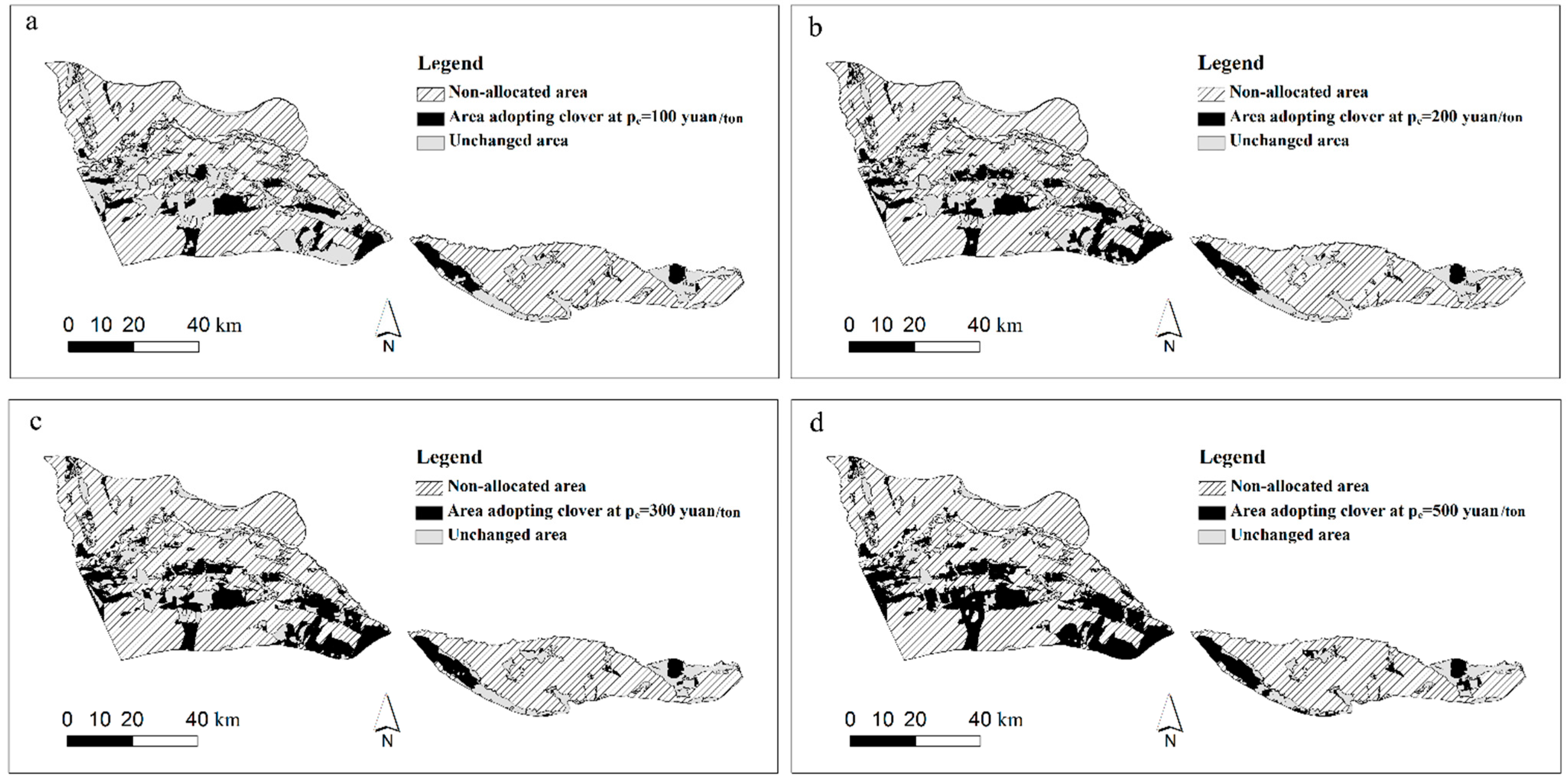
3.1.3. Land Use Reallocation with the Tradeoff Analysis

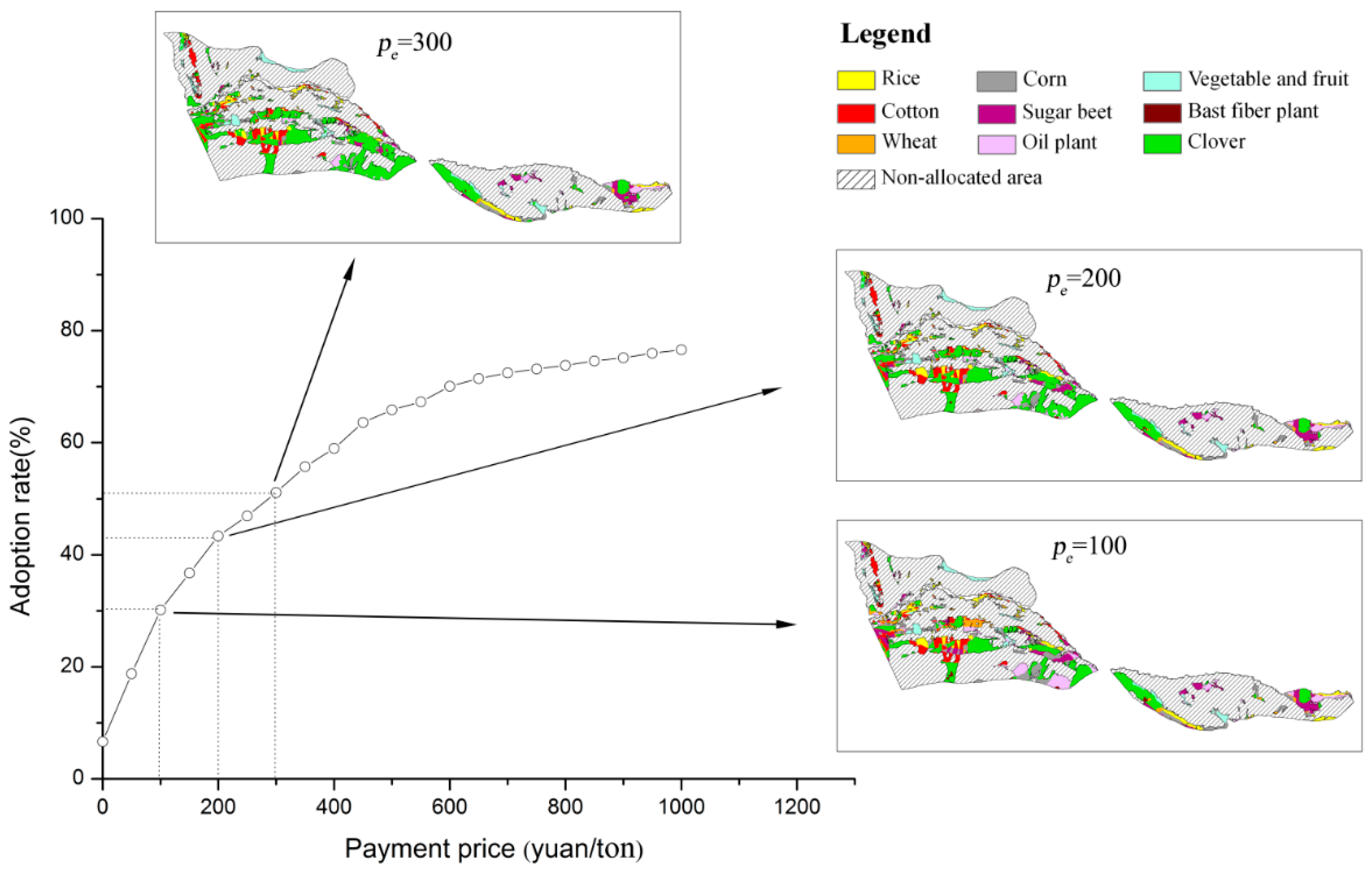
For land use planning, it is often useful to indicate to policy makers the spatial variations where payment policy is likely to be adopted by farmers, in addition to actual aggregated adoption rates. This means areas where opportunity costs go from positive to negative with each payment price can be identified, and are therefore reallocated to clover. Using the spatial distributions of adopting clover in Figure 6, the origin land use scenario is reallocated to clover at each payment price. Then the area of each crop at different payment prices can be calculated. Table 3 shows several examples of areas for each crop under different scenarios. As the payment price increases, areas planted with other crops decrease with different change rates except for vegetables and fruit. Areas that are planted with crops with relatively low net returns and that would supply high ecosystem service values by changing crops to clover would easily adopt the payment policy. Therefore, areas planting the bast fiber plant and wheat turn to clover at this relatively low payment price. In contrast, areas planted with cotton, vegetables, and fruit would not easily adopt clover. In particular, areas of vegetables and fruit do not change even when the payment price is up to 500 yuan/ton.

Figure 7 shows examples of spatial reallocation maps at payment prices of 100, 200, and 300 yuan/ton. It shows that areas starting to change to clover at a payment price of 100 yuan/ton are located in the south of the newly reclaimed region. These areas majorly planted with sugar beet, the bast fiber plant, and wheat would also supply high ecosystem service values when turning to clover. The western region starts to adopt the payment policy when the payment price is up to 200 yuan/ton. Also, areas planted with sugar and corn, two crops with high net returns, start to change to clover because of high payments. Such maps can show decision makers where clover would be adopted at a specific payment price. All such information assists in site selection, payment policy implementation, and planning effectiveness evaluation.

Figure 7. Changes in adoption rates and payment prices in the tradeoff curve with the corresponding land use reallocation map.

Figure 7. Changes in adoption rates and payment prices in the tradeoff curve with the corresponding land use reallocation map.

Table 3. Simulated area of each crop with different payment prices (10⁴ ha).

Payment price (yuan/ton)	Reference scenario	pe = 50	pe = 100	pe = 150	pe = 200	pe = 250	pe = 300	pe = 350	pe = 400	pe = 450	pe = 500
Wheat	3.08	2.01	1.16	0.78	0.47	0.38	0.31	0.20	0.13	0.11	0.10
Corn	2.41	2.36	2.02	1.84	1.61	1.51	1.25	1.11	1.05	0.93	0.87
Rice	1.23	1.16	1.16	1.16	1.16	1.12	1.05	0.91	0.84	0.83	0.80
Cotton	1.48	1.36	1.36	1.36	1.36	1.36	1.36	1.36	1.27	0.86	0.73
Sugar beet	1.68	1.52	1.52	1.40	1.21	1.05	0.96	0.86	0.76	0.73	0.68
Oil plant	0.81	0.75	0.73	0.58	0.45	0.40	0.35	0.25	0.21	0.20	0.19
Bast fiber plant	0.62	0.35	0.08	0.05	0.04	0.02	0.01	0.00	0.00	0.00	0.00
Vegetables and fruit	1.09	1.09	1.09	1.09	1.09	1.09	1.09	1.09	1.09	1.09	1.09
Clover	0.65	2.45	3.93	4.79	5.66	6.12	6.67	7.27	7.70	8.30	8.59

Table 3. Simulated area of each crop with different payment prices (10⁴ ha).

Payment price (yuan/ton)	Reference scenario	pe = 50	pe = 100	pe = 150	pe = 200	pe = 250	pe = 300	pe = 350	pe = 400	pe = 450	pe = 500
Wheat	3.08	2.01	1.16	0.78	0.47	0.38	0.31	0.20	0.13	0.11	0.10
Corn	2.41	2.36	2.02	1.84	1.61	1.51	1.25	1.11	1.05	0.93	0.87
Rice	1.23	1.16	1.16	1.16	1.16	1.12	1.05	0.91	0.84	0.83	0.80
Cotton	1.48	1.36	1.36	1.36	1.36	1.36	1.36	1.36	1.27	0.86	0.73
Sugar beet	1.68	1.52	1.52	1.40	1.21	1.05	0.96	0.86	0.76	0.73	0.68
Oil plant	0.81	0.75	0.73	0.58	0.45	0.40	0.35	0.25	0.21	0.20	0.19
Bast fiber plant	0.62	0.35	0.08	0.05	0.04	0.02	0.01	0.00	0.00	0.00	0.00
Vegetables and fruit	1.09	1.09	1.09	1.09	1.09	1.09	1.09	1.09	1.09	1.09	1.09
Clover	0.65	2.45	3.93	4.79	5.66	6.12	6.67	7.27	7.70	8.30	8.59

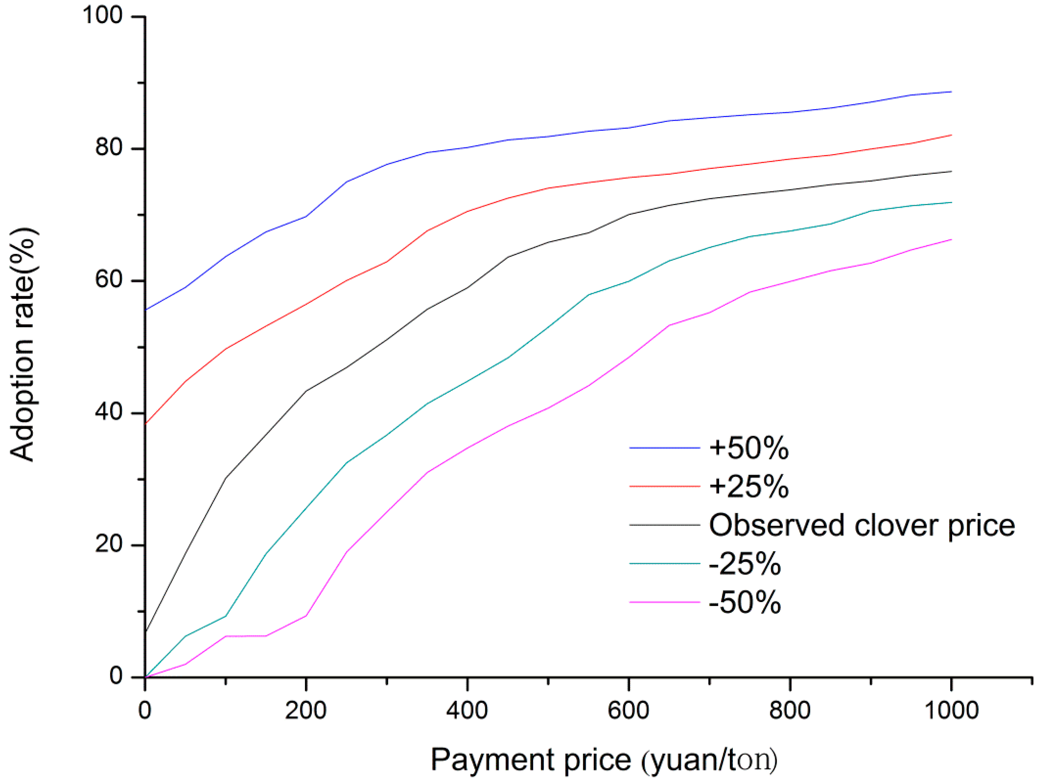
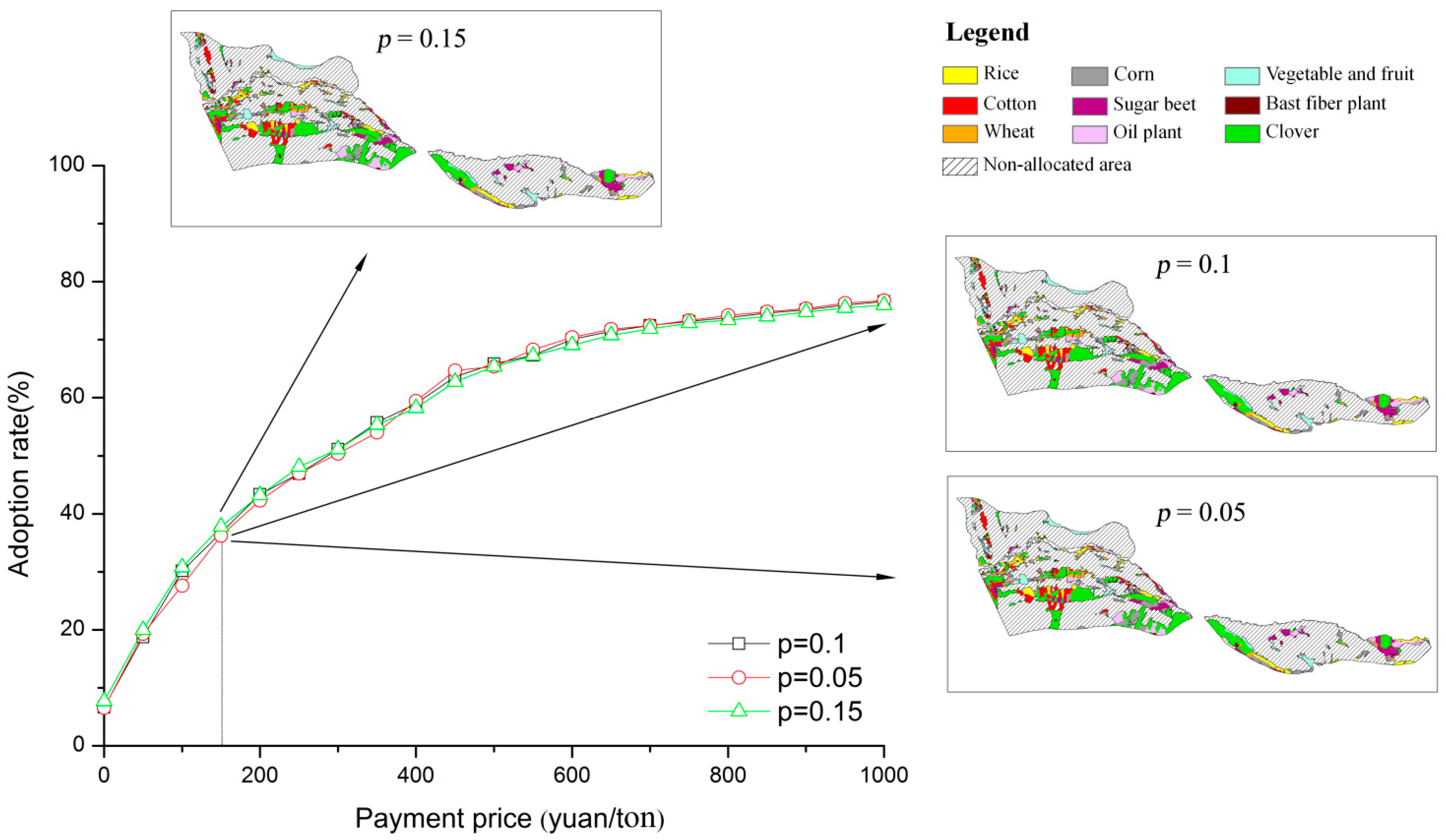
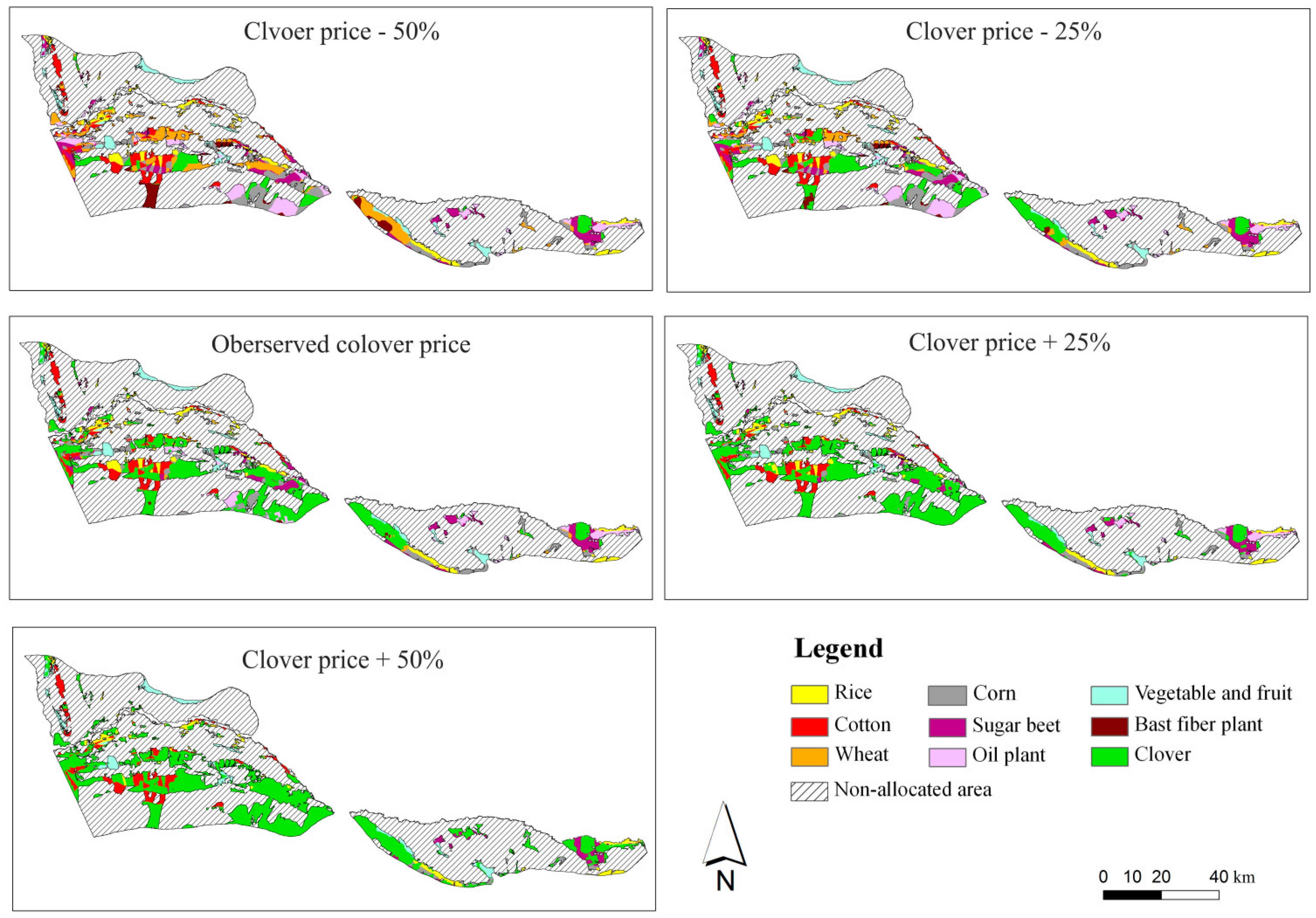
3.2. Sensitivity Analysis for the Tradeoff Analysis

The S-membership function was used to link LSE and crop yield, but the key parameters (α and γ) are not available from the household survey and statistical data. The α and γ are the ideal limits of crop yields at local conditions; we can only collect the highest and lowest crop yields (x_h, and x_l), which are not up to the lower and upper limit but are close to α and γ. Then we proposed parameter p to calculate the α and γ. With Equation (5), the membership value of x_l is p and (1 – p) is the membership for the x_h. There are no long-term locally measured data available to calibrate the results. A sensitivity analysis was performed for parameter p to indicate the uncertainty of the model output.

Based on the origin setting (p = 0.1), we set the p ± 50% as p = 0.05 and p = 0.15, and two tradeoff curves were generated. The corresponding land use spatial reallocation maps were displayed and compared with the original result (Figure 8). The three tradeoff curves appear very similar, and reallocated land use maps are likely similar with a payment price of 150 yuan/ton. With this payment price, the adoption rates are 36.2%, 36.7%, and 37.5% for p = 0.05, p = 0.05, and p = 0.15, respectively. When parameter p changes, simulated yields for individual crops change, and a smaller p value will generate a smaller range for the yield and net return of each crop. However, the relative gap between different crops is stable at each site. The range of opportunity costs also remains stable, although the upper and lower limits change. For example, rather than the opportunity costs without payments of p = 0.1 (ranging from −1557 to 28,950 yuan/ha), results of p = 0.05 and p = 0.15 are −1395 to 27,988.5 yuan/ha and −2743.5 to 30,064.5 yuan/ha, respectively. This indicates that the tradeoff analysis based on the opportunity costs of different crops is robust when parameter p changes. Also, it demonstrates that the output of the ALUOA-TOA system is robust in our case study.

Figure 8. Sensitivity analysis for tradeoff analysis with the corresponding spatial map at different p values.

Figure 8. Sensitivity analysis for tradeoff analysis with the corresponding spatial map at different p values.

As prices of crops vary in the future, a sensitivity analysis on crop prices would illustrate the performance of our method. Although nine crops were simulated in our case study, we only changed the price of clover as an example of the sensitivity analysis, which would easily change the opportunity costs in the whole area. If prices of other crops change, they would similarly change opportunity costs in specific areas with the corresponding crop. Five scenarios were defined: two with 50% and 25% increase in mean clover price, one with the observed clover price, and two with a 25% and 50% decrease in mean clover price.

Figure 9 shows five tradeoff curves with the above settings for the sensitivity analysis. It indicates that the clover price would significantly change outputs of the method. Without payments, the adoption rates for the five scenarios are significantly different. The study area would not adopt clover because of low net returns when the clover price decreases by 25% and 50%. In contrast, more areas would adopt clover as an economic incentive when the clover price increases by 25% and 50%. Figure 10 displays corresponding land use maps at different clover prices with p_e = 200 yuan/ton. When the clover price decreases by 50%, only limited areas adopt the payment policy. If the clover price decreases by 25%, more areas would select clover. When the payment price increases by 25% and 50%, the adoption rates exceed 50%. When the payment price increases, the gaps of adoption rates in the five scenarios will be narrow. This is because larger payments would change opportunity costs in major areas from positive to negative and stimulate farmers to adopt the payment policy even with low clover price. As mentioned above, our method assumes that farmers make land use decisions to maximize their perceived economic incomes. Then the price of crops would significantly affect farmers’ net returns without payments and farmers’ selection of crops. This shows that our method and outputs can reflect the sensitivity of this key parameter. When prices of crops change, we should make a new ex ante analysis of the tradeoff between ecosystem service benefits and environmental compensation costs to set a reasonable payment price.

Figure 9. Sensitivity analysis for tradeoff curves at different clover prices.

Figure 9. Sensitivity analysis for tradeoff curves at different clover prices.

Figure 10. Spatial land use maps at different clover prices with p_e = 200 yuan/ton.

Figure 10. Spatial land use maps at different clover prices with p_e = 200 yuan/ton.

4. Discussion

4.1. Advantage of Spatially Explicit Tradeoff Analysis on Sustainable Land Use Planning

Sustainable land use allocation planning not only must realize as many economic benefits as possible, but must protect environmental integrity and public health. In this study, we developed the ALUOA-TOA system to support sustainable land use planning, applied it in the newly reclaimed region of Yili, and validated its usefulness. Supplementing the TOA-MD [14,15,16,17,18], our tool established spatial distribution of land use allocation for the tradeoff curve at each corresponding payment price, which provides more detailed information for decision making.

Relative to traditional land use allocation [7,8,20], our tool integrates the tradeoff analysis to evaluate the effectiveness of land use planning with payment policy, and its economic feasibility. Land use planning, which takes into account economic benefits to farmers, can be achieved by providing farmers with incentives for ecosystem services rather than government mandates or appeals to idealism. In previous studies, the TOA-MD is a comparison between two land use systems. To calculate the parameters of the model if the land use system is not composed of individual activities, a weight summation method is used to combine multiple activities [17,38]. The advantage with our tool is that it can perform tradeoff analysis between different land use types without the summation method. This capability is more suitable for small and fragmented farms in China.

4.2. Uncertainties of Tradeoff Analysis

It should be noted that the adoption rate produced by the tradeoff model is the upper limit at each specific payment price, consistent with the TOA-MD system [14,15,16,17,18]. To develop a low-cost, rapid ex ante method, the model is based on an assumption of economic incentive (expected profitability), rather than other possible mechanisms to change farmer behavior, similar to the TOA-MD [14,15,16,17,18], such as costs differentials between land uses [18,38], risk aversion, household consumption preferences [17], and other non-economic factors driving decision-making behavior [38]. It would be useful to examine, through additional intensive household surveys, other determinants of farmer decision making, and perhaps establish a more accurate adoption rate if the above data on farmers’ behavior factors are available.

The accuracy for policy analysis is arguably lower than that for scientific research because ex ante policy analysis involves a large number of uncertainties that cannot be quantified [18]. We used the S-membership function to simulate potential crop yields [23,27] if household survey data for the spatial characteristic are insufficient—an acceptable method for ex ante analysis. The LSE, based on high mean and low crop yields from limited field data and statistical yearbooks, was used to generate the spatial distribution of crop yields. It is a crucial step in the ALUOA system, but also the key link in our ALUOA-TOA system. With the S-membership function, our tool simulates crop yields at a low cost, based on the LSE without other simulation models for additional parameters [39,40,41]. Sensitivity analysis of our tool as applied in this case study has also validated the robustness of the system (Figure 7). We assumed that the management intensity of the same crop was the same, which is acceptable as an ex ante analysis for land planning in the newly reclaimed area.

On the other hand, our tool estimated the supply of ecosystem service values as the decrease in soil erosion from changing other crops to clover. In our case study, the ecosystem service value of clover is much larger than other land use types and clover will do much better than other crops to prevent land degradation in the Yili region. Except for rice, we assumed that ecosystem service values for changing crops to clover are the same if done at the same site. The decrease in soil erosion differentials for various land use types and other types of ecosystem service values can be evaluated in a future study. Because our land use allocation planning approach was not implemented in the study region, it needs elaborate data from site-specific surveys to validate assumptions and simplifications in the system. Also, management difference can be included in the crop yield estimation in a future study.

Our ALUOA-TOA system can allocate crop types on a spatial distribution map based on payment policy. It requires further case studies to confirm its validity for sustainable agriculture, and to explore its role in supporting decision making and policy development. In future studies it would also be useful to examine additional farmer behavior factors, as well as limitations of the model, in part to balance the estimation costs of parameters estimation and the prediction accuracy of the model.

5. Conclusions

The land use optimal allocation process, coupled with a payment policy for ecosystem services, is useful in land use planning for sustainable agriculture. We developed a spatially explicit, low-cost tool that integrates tradeoff analysis with a land use optimal allocation system, which was an ex ante evaluation of payment policy and reallocated the land use map. The application of our ALUOA-TOA system in the newly reclaimed region of Yili demonstrated how it worked in land use planning and decision making. Based on the spatial LSE, the method used S-membership functions to estimate potential crop yields and simulate the opportunity costs of farmers changing origin crops to clover under the payment policy. With each payment price, farmers’ adoption rate of clover was simulated, generating a tradeoff curve. Areas where farmers adopted the payment policy and changed the origin land use were identified and were reallocated on a basic land use allocation map. Our approach assessed a tradeoff between the origin land use and the target land with payments for farmers. Also, the government could assign a reasonable payment price between ecosystem services and economic costs for the tradeoff analysis. The results demonstrated that our approach provides additional detailed information for decision making; modifications to improve our tool could be explored in future studies.

References

1. Tilman, D.; Cassman, K.G.; Matson, P.A.; Naylor, R.; Polasky, S. Agricultural sustainability and intensive production practices. Nature 2002, 418, 671–677. [Google Scholar] [CrossRef] [PubMed]
2. Godfray, H.C.J.; Beddington, J.R.; Crute, I.R.; Haddad, L.; Lawrence, D.; Muir, J.F.; Pretty, J.; Robinson, S.; Thomas, S.M.; Toulmin, C. Food security: The challenge of feeding 9 billion people. Science 2010, 327, 812–818. [Google Scholar] [CrossRef] [PubMed]
3. Robertson, G.P.; Swinton, S.M. Reconciling agricultural productivity and environmental integrity: A grand challenge for agriculture. Front. Ecol. Environ. 2005, 3, 38–46. [Google Scholar] [CrossRef]
4. Pretty, J. Agricultural sustainability: Concepts, principles and evidence. Philos. Trans. R. Soc. B Biol. Sci. 2008, 363, 447–465. [Google Scholar] [CrossRef]
5. Liu, Y.; Wang, H.; Ji, Y.; Liu, Z.; Zhao, X. Land use zoning at the county level based on a multi-objective particle swarm optimization algorithm: A case study from Yicheng, China. Int. J. Environ. Res. Public Health 2012, 9, 2801–2826. [Google Scholar] [CrossRef] [PubMed]
6. Santé-Riveira, I.; Boullón-Magán, M.; Crecente-Maseda, R.; Miranda-Barrós, D. Algorithm based on simulated annealing for land-use allocation. Comp. Geosci. 2008, 34, 259–268. [Google Scholar] [CrossRef]
7. Cao, K.; Huang, B.; Wang, S.; Lin, H. Sustainable land use optimization using Boundary-Based Fast Genetic Algorithm. Comp. Environ. Urban Syst. 2012, 36, 257–269. [Google Scholar] [CrossRef]
8. Gong, J.; Liu, Y.; Chen, W. Optimal land use allocation of urban fringe in Guangzhou. J. Geogr. Sci. 2012, 22, 179–191. [Google Scholar] [CrossRef]
9. Wang, S.-H.; Huang, S.-L.; Budd, W.W. Integrated ecosystem model for simulating land use allocation. Ecol. Model. 2012, 227, 46–55. [Google Scholar] [CrossRef]
10. Crissman, C.C.; Antle, J.M.; Capalbo, S.M. Economic, Environmental, and Health Tradeoffs in Agriculture: Pesticides and the Sustainability of Andean Potato Production; International Potato Center: Dordrecht, The Netherlands, 1998. [Google Scholar]
11. Antle, J.M.; Stoorvogel, J.J.; Crissman, C.C.; Bowen, W. Tradeoff Assessment as a Quantitative Approach to Agricultural/Environmental Policy Analysis. In Proceedings of the SAAD III Third International Symposium on Systems Approaches for Agricultural Development, Lima, Peru, 8–10 November 1999.
12. Stoorvogel, J.; Antle, J.M.; Crissman, C.; Bowen, W. The tradeoff analysis model: Integrated bio-physical and economic modeling of agricultural production systems. Agric. Syst. 2004, 80, 43–66. [Google Scholar] [CrossRef]
13. Antle, J.; Stoorvogel, J.; Bowen, W.; Crissman, C.; Yanggen, D. The tradeoff analysis approach: Lessons from Ecuador and Peru. Q. J. Int. Agric. 2003, 42, 189–206. [Google Scholar]
14. Immerzeel, W.; Stoorvogel, J.; Antle, J. Can payments for ecosystem services secure the water tower of Tibet? Agric. Syst. 2008, 96, 52–63. [Google Scholar] [CrossRef]
15. Claessens, L.; Antle, J.; Stoorvogel, J.; Valdivia, R.; Thornton, P.; Herrero, M. A method for evaluating climate change adaptation strategies for small-scale farmers using survey, experimental and modeled data. Agric. Syst. 2012, 111, 85–95. [Google Scholar] [CrossRef] [Green Version]
16. Jack, B.K.; Leimona, B.; Ferraro, P.J. A revealed preference approach to estimating supply curves for ecosystem services: Use of auctions to set payments for soil erosion control in Indonesia. Conserv. Biol. 2009, 23, 359–367. [Google Scholar] [CrossRef] [PubMed]
17. Antle, J.M.; Diagana, B.; Stoorvogel, J.J.; Valdivia, R.O. Minimum-data analysis of ecosystem service supply in semi-subsistence agricultural systems. Aust. J. Agric. Resour. Econ. 2010, 54, 601–617. [Google Scholar] [CrossRef]
18. Antle, J.M.; Valdivia, R.O. Modelling the supply of ecosystem services from agriculture: A minimum-data approach. Aust. J. Agric. Resour. Econ. 2006, 50, 1–15. [Google Scholar] [CrossRef]
19. Kang, L.; Zhang, H. Assessment of the Land Desertification Sensitivity of Newly Reclaimed Area in Yili, Xinjiang. Resour. Sci. 2012, 34, 896–902. (In Chinese) [Google Scholar]
20. Zhang, Y.; Zhang, H.; Ni, D.; Song, W. Agricultural land use optimal allocation system in developing area: Application to Yili watershed, Xinjiang Region. Chin. Geogr. Sci. 2012, 22, 232–244. [Google Scholar] [CrossRef]
21. Shi, Y. Opinions on the land development in Yili region. Xinjiang Agric. Sci. 2008, 45, 1–3. [Google Scholar]
22. Food and Agriculture Organisation (FAO). A Framework for Land Evaluation (Soils Bulletin No. 32); Food and Agriculture Organisation of the United Nations: Rome, Italy, 1976. [Google Scholar]
23. Rossiter, D.G. A theoretical framework for land evaluation. Geoderma 1996, 72, 165–190. [Google Scholar] [CrossRef]
24. Nisar Ahamed, T.; Gopal Rao, K.; Murthy, J. GIS-based fuzzy membership model for crop-land suitability analysis. Agric. Syst. 2000, 63, 75–95. [Google Scholar]
25. Kalogirou, S. Expert systems and GIS: An application of land suitability evaluation. Comp. Environ. Urban Syst. 2002, 26, 89–112. [Google Scholar] [CrossRef]
26. Verheye, W. Land evaluation. In Land Use, Land Cover and Soil Sciences; UNESCO-EOLSS Publishers: Oxford, UK, 2008. [Google Scholar]
27. Dumanski, J.; Onofrei, C. Techniques of crop yield assessment for agricultural land evaluation. Soil Use Manag. 1989, 5, 9–15. [Google Scholar] [CrossRef]
28. Tang, H.; Debaveye, J.; Ruan, D.; van Ranst, E. Land suitability classification based on fuzzy set theory. Pedologie 1991, 41, 277–290. [Google Scholar]
29. Keshavarzi, A.; Sarmadian, F.; Ahmadi, A. Spatially-based model of land suitability analysis using Block Kriging. Aust. J. Crop Sci. 2011, 5, 1533–1541. [Google Scholar]
30. Samranpong, C.; Ekasingh, B.; Ekasingh, M. Economic land evaluation for agricultural resource management in Northern Thailand. Environ. Model. Softw. 2009, 24, 1381–1390. [Google Scholar] [CrossRef]
31. Van Ranst, E.; Tang, H.; Groenemam, R.; Sinthurahat, S. Application of fuzzy logic to land suitability for rubber production in peninsular Thailand. Geoderma 1996, 70, 1–19. [Google Scholar]
32. Costanza, R.; d’Arge, R.; de Groot, R.; Farber, S.; Grasso, M.; Hannon, B.; Limburg, K.; Naeem, S.; O’Neill, R.V.; Paruelo, J.; et al. The value of the world’s ecosystem services and natural capital. Nature 1997, 387, 253–260. [Google Scholar] [CrossRef]
33. Kinnell, P. Event soil loss, runoff and the Universal Soil Loss Equation family of models: A review. J. Hydrol. 2010, 385, 384–397. [Google Scholar] [CrossRef]
34. Cai, C.; Ding, S.; Shi, Z.; Huang, L.; Zhang, G. Study of Applying USLE and Geographical Information System IDRISI to Predict Soil Erosion in Small Watershed. J. Soil. Water Conserv. 2000, 14, 19–24. (In Chinese) [Google Scholar]
35. Geospatial Data Cloud. http://www.gscloud.cn/ (accessed on 25 November 2014).
36. Data Sharing Infrastructure of Earth System Science. http://www2.geodata.cn/data/dataresource.html (accessed on 25 November 2014).
37. Yili Municipal Bureau of Statistics. Yili Kazakh Autonomous Prefecture Statistical Yearbook; Yili Municipal Bureau of Statistics: Xinjiang, China, 2007. [Google Scholar]
38. Claessens, L.; Stoorvogel, J.; Antle, J.M. Ex ante assessment of dual-purpose sweet potato in the crop-livestock system of western Kenya: A minimum-data approach. Agric. Syst. 2008, 99, 13–22. [Google Scholar] [CrossRef]
39. Williams, J.R.; Singh, V. The EPIC Model. In Computer Models of Watershed Hydrology; Water Resources Publisher: Colorado, CO, USA, 1995; pp. 909–1000. [Google Scholar]
40. Keating, B.A.; Carberry, P.; Hammer, G.; Probert, M.E.; Robertson, M.; Holzworth, D.; Huth, N.; Hargreaves, J.; Meinke, H.; Hochman, Z. An overview of APSIM, a model designed for farming systems simulation. Eur. J. Agron. 2003, 18, 267–288. [Google Scholar] [CrossRef]
41. Jones, J.W.; Hoogenboom, G.; Porter, C.; Boote, K.; Batchelor, W.; Hunt, L.; Wilkens, P.; Singh, U.; Gijsman, A.; Ritchie, J. The DSSAT cropping system model. Eur. J. Agron. 2003, 18, 235–265. [Google Scholar] [CrossRef]