

Contrastive Analysis and Accuracy Assessment of Three Global 30 m Land Cover Maps Circa 2020 in Arid Land

1
Faculty of Geomatics, Lanzhou Jiaotong University, Lanzhou 730070, China
2
National-Local Joint Engineering Research Center of Technologies and Applications for National Geographic State Monitoring, Lanzhou 730070, China
*
Author to whom correspondence should be addressed.
Sustainability 2023, 15(1), 741; https://doi.org/10.3390/su15010741
Submission received: 1 November 2022
/
Revised: 3 December 2022
/
Accepted: 6 December 2022
/
Published: 31 December 2022
(This article belongs to the Special Issue Application of Remote Sensing for Sustainable Development)
Abstract
:Fine-resolution land cover (LC) products are critical for studies of urban planning, global climate change, the Earth’s energy balance, and the geochemical cycle as fundamental geospatial data products. It is important and urgent to evaluate the performance of the updated global land cover maps. In this study, three widely used LC maps with 30 m spatial resolution (FROM-GLC30-2020, GLC_FCS30, and GlobeLand30) published around 2020 were evaluated in terms of their degree of consistency and accuracy metrics. First, we compared their similarities and difference in the area ratio and spatial patterns over different land cover types. Second, the sample and response protocol was proposed and validation samples were collected. Based on this, the overall accuracy, producer’s accuracy, and user’s accuracy were analyzed. The results revealed that: (1) the consistent areas of the three maps accounted for 65.96% of the total area and that two maps exceeded 75% of it. (2) The dominant land cover types, bare land and grassland, were the most consistent land cover types across the three products. In contrast, the spatial inconsistency of the wetland, shrubland, and built-up areas were relatively high, with the disagreement mainly occurring in the heterogeneous regions. (3) The overall accuracy of the GLC_FCS30 map was the highest with a value of 87.07%, which was followed by GlobeLand30 (85.69%) and FROM-GLC30 (83.49%). Overall, all three of the LC maps were found to be consistent and have a good performance in classification in the arid regions, but their ability to accurately classify specific types varied.
1. Introduction
Global land cover (LC) products used by the scientific community, international organizations, and the government sector are critical to the understanding of global climate change [1], land cover change [2], environmental pollution [3], food security [4], ecological conservation, and the coordination of actions aiming to achieve the sustainable development goals (SDGs) [5]. Meanwhile, the Global LC data are vital information sources for studying the complex interactions between the human activities and the global changes [6].
The first satellite-based global LC map dates to the 1990s [7]. Since then, with the improvement of satellite techniques and computer facilities, various global/regional land cover maps with different resolutions based on specific classification schemes have been developed and released. Several types of LC maps with a relatively coarse resolution at the 1000 and 300 m scales [8,9,10,11,12,13] are available. While the coarser resolution global LC maps have provided valuable information for various related applications, some studies [14,15] pointed out that these products cannot meet the requirement of accuracy in regions with heterogeneous landscapes, which calls for there to be a finer resolution and more accurate data in these areas.
Recently, due to the free availability of finer resolution remotely sensed imagery from the constellations of Landsat and Sentinel, finer resolution maps were produced, such as: (1) FROM30, the Finer Resolution Observation and Monitoring Global LC dataset based on Landsat images, which has a 30 m resolution [16], (2) Globeland30, the global land cover dataset from National Geomatics Center of China from 2000/2010, which has a 30 m resolution [17], (3) GLC_FCS30, the global land cover product with a fine classification system that works at 30 m using time-series Landsat imagery from 2015, which has a 30 m resolution [18,19], (4) FROM-GLC10, the Finer Resolution Observation and Monitoring Global LC dataset based on Landsat images, which has a 10 m resolution [20], (5) ESA WorldCover10, a new baseline global land cover product at a 10 m resolution based on Sentinel-1 and -2 data from the European Space Agency (ESA) from 2020, which has a 10 m resolution [21,22], and (6) ESRI10, the New 2020 Global Land Cover Map from Esri [23]. In contrast to the 10 m resolution LC, the 30 m resolution global LC maps such as GlobeLand30, GLC_FCS30, and FROM30 are commonly used in many fields because of their long time series and robustness in land cover mapping [17,18,24,25,26].
However, the LC maps mentioned above are classified from multi-source remote sensed data using different classification methods and classification schemes and there must be incompatibility and uncertainties among these datasets. The quality of the LC products is an extensive issue that may relate to a variety of their properties and the property of interest is the thematic classification accuracy. Therefore, the methods proposed for assessing the thematic performance of the LC data that are commonly used are: (1) a comparison analysis of statistical or spatial consistency with existing LC maps or government statistical data [27] and (2) quantifying the accuracies through error metrics, including the overall accuracy (OA), user’s accuracy (UA), and product’s accuracy (PA) derived from an error matrix constructed by a reference dataset [28].
Most of the studies are focused on the performance of classifications, that is, the accuracy assessment of the LC maps [29]. Seven global LC datasets with resolutions ranging from 30 to 1000 m over China were assessed by the error matrix method [30]. Over Europe, an accuracy assessment of three 30 m LC products circa 2015 was conducted using the LUCAS reference dataset and the overall accuracy varied from 65.3 to 84.33% [27]. Tsendbazar et al. (2018) generated a validation dataset including 3617 sample sites in Africa based on stratified sampling via the Geo-Wiki platform and validated the newly released 100 m resolution LC products from the Copernicus Global Land Service (CGLS-LC100). On a global scale, the producer of GlobeLand30 first developed an online validation system, GLCVal, and it provided an accuracy assessment of GlobeLand30 for about 20 countries (regions) [24].
Parts of the studies have concentrated on specific classes that dominated or played an important role in a specific area, such as cropland, forest, or waterbody areas. Zhang et al. (2022) implemented a comparison analysis and an accuracy assessment for six 30 m resolution cropland products based on more than 30,000 ground truth points collected in a visual interpretation study in China [31,32]. Lu et al. [33] compared five global cropland datasets circa 2010 in China and they concluded that the GlobeLand30 is better than the other four products are in terms of the accuracies of the cropland area and spatial location. Xing et al. [34] explored the accuracy, consistency, and discrepancies of eight widely used forest datasets in Myanmar and analyzed the factors influencing the spatial consistency from the aspects of terrain and climate.
The latest version of FROM-GLC30 was released in 2018 and the newest version of GlobeLand30 and GLC_FCS30 were both released in 2020. For a short time, since the release of these 30 m resolution LC map datasets, the performance of these LC datasets has still been insufficient. Therefore, it is urgent to conduct the comparative analysis and accuracy assessment of the latest LC maps. The landscapes in arid areas are complex and diverse and some of the literature studies have reported low accuracies [30,32]. The ecological environment is fragile due to a shortage of water resources. With the increase in the population, the continuous development of the oasis in the arid regions has resulted in severe ecological and environmental problems, such as water shortages, vegetation degradation, desertification, and salinization [33,34,35]. However, a few comparative analyses and accuracy assessments of 30 m LC products in arid regions have been conducted. Therefore, it is very essential to assess the accuracy and spatial consistency of different LC maps in arid areas.
Overall, there are still research gaps in the current evaluation works: (1) the local performance cannot be represented by the global accuracy due to the spatial inconsistency of the LC, particularly in an arid area. A global estimation for the entire map may be inappropriate for the sub-regions for the same reason, the baseline samples used by the map producers will not be large enough for regional and class-specific accuracy estimates [36] and (2) there is a lack of consistency in analyses among the different LC maps. Compared to many previous studies dedicated to the validation of existing LC maps, a few attempts have been performed to conduct spatial and statistical consistency analyses and (3) the absence of some issues determined the accuracy.
The present paper aimed to compare and validate three widely used global LC maps in arid land over Northwest China, including FROM30, GLC_FCS30, and GlobeLand30, in the terms of areal similarity, spatial consistency, and qualitative accuracy through error matrices. The study results can guide future improvements of LC mapping. Moreover, they also provide advice for users to select the best LC map in arid regions.
2. Materials and Methodology
2.1. Study Area
The study area belongs to the northwest of China, located between longitudes 73°20′–111°7′ E and latitudes 31°30′–49°10′ N, with a total area of 3.08 × 10⁶ km2. Northwestern China, including the Shaanxi Province, Ningxia Hui Autonomous Region, Gansu Province, Qinghai Province, and Xinjiang Uygur Autonomous Region (Shaanxi, Ningxia, Qinghai, Gansu, and Xinjiang for short), covers a vast area characterized by mountain ranges, plateaus, and basins with varied landforms, as shown in Figure 1. Northwestern China is characterized by a dry climate, which results in a harsh ecological environment, very low vegetation coverage, and very small amount of water vapor evaporation. The annual precipitation here is below 400 mm, or even less than 50 mm in the desert, which occupies a large proportion of the area [37]. The rivers are mainly supplied by snow melt water in the mountainous areas and belongs to internal rivers. Due to the variety of landforms, the LC types in this region are complex and diverse, the most widely distributed types being desert, grassland, and cropland.
2.2. The 30 m Global LC Datasets
In the present study, three widely used LC maps that are available freely were chosen for evaluation and analysis. These are the Finer Resolution Observation and Monitoring Global LC datasets based on Landsat images in 2017 (abbr. FROM), available at: http://data.ess.tsinghua.edu.cn [16], Global land cover datasets in 2020 from National Geomatics Center of China (abbr. Globe), available at: www.globallandcover.com [17], and global land cover product with fine classification system at 30m using time-series Landsat imagery in 2020, (abbr. FCS) available at: https://doi.org/10.5281/zenodo.3986872 [18,19]. All three of the datasets were downloaded in May 2022.
The FROM V2017 is the latest product of FROM_GLC30 data series with 30 m resolution global LC maps. In this study, we selected the FROM released in 2018 for evaluation and conducted a consistency analysis and accuracy assessment based on 10 first-level types. The Globe V2020 is a successor to the previous versions named GlobeLand30 V2000 and GlobeLand30 V2010, which was released in 2020 [17]. It uses a classification system containing 10 first-level types. The accuracy evaluation of Globe was conducted by the producer, the overall accuracy of Globe data was 85.72%, and the Kappa coefficient was 0.82 [18].
FCS30 V2020 is successor to GLC_FCS30-2015, combining with 2019–2020 time series remote sensed data, such as Landsat multispectral images, sentinel SAR data, global thematic auxiliary dataset, and interpreted training samples [19]. It adopted the classification system that consists of nine first-level types and 30 s-level types [19]. The GLC_FCS-2015 was validated using 44,043 validation samples and reported an overall accuracy of 82.5% and a Kappa coefficient of 0.784 for the level-0 validation system (9 basic land cover types). The main parameters of the three LC maps are listed in Table 1.
2.3. Harmonization of the Classification Systems
The basic processing method mainly included raster data clipping, projection transformation, and harmonization of classification schemes among the different LC maps. The coordinates of LC maps were unified to WGS84 coordinate and Universal Transverse Mercator projection. There were significant discrepancies among the classification schemes adopted by the three LC maps. FROM and FCS had a two-level hierarchical classification scheme with 10 and 9 first-level types, respectively. Globe had 10 basic land cover types, which were the same as the first-level classification system used in FROM.
In the comparative evaluation of the different LC products, it was essential to unify the discrepant classification schemes into the same classification scheme to reduce errors. Based on the user manuals of the three 30 m LC products [16,18,25], a merged classification scheme with nine major LC types, including cropland, forest, grassland, shrubland, wetland, water, built-up, bare land, and permanent snow/ice was designed (Table 2). The most classes could be directly assessed to merged types. In particular, the types of tundra in the FROM and Globe were merged into shrubland and the types in FCS second-level were combined into FCS first-level according to the producer’s hierarchical classification system [18]. In addition, the cloud cover pixels occupied a small proportion in the FROM map and thus were ignored.
2.4. Consistency Analysis
To present a rounded analysis between the three 30 m newly released LC products, the consistency analysis from two aspects (area-based consistency and pixel-based consistency) was conducted. The area-based consistency analysis points out the area similarity of the types. The pixel-based consistency focused on the consistency of LC maps at the locations. Although the presented time of FROM is 3 years ahead of that for Globe and FCS of 2020, some studies have concluded that the LC changes that occurred over this time interval were almost negligible compared to the classification error in the LC products [18].
2.4.1. Area-Based Consistency for LC Products
The area-based consistency focused on the difference in aerial proportions of each LC type between different LC maps. The areas of each LC type in different maps were compared, which could visually demonstrate the consistency and diversity of different LC products.
2.4.2. Pixel-Based Consistency
The pixel-based consistency concerned the spatial (in)consistency for each LC type and the spatial superposition method was employed to obtain the pixel-based consistency. The overall similarity coefficient (OS) and the class similarity coefficient (CS) between different products were calculated using Equations (1) and (2) [21,27]:
where Xi is the number of pixels of the i-th LC type in map X, Yi is the number of pixels of the i-th LC type in map Y, is the number of pixels of the i-th LC type in both X and Y, and n is the number of classes used to calculate the overall spatial agreement, here nine, and M is the total number of pixels in the study area. Equation (2) is also applicable to the consistent operation of three or more layers.
The superposition results between two LC products presented a binary structure: inconsistent and consistent (Figure 3a) and provided a ternary or multivariate structure among three or more LC products as well (Figure 3b). In this study, no more than three LC products were overlaid, so there were three levels as follows in descending order: (1) consistent: the classes of the three LC products were same at a given pixel; (2) basically consistent: any two LC products had the same type at a given pixel; and (3) inconsistent: all the three LC maps had different types at a specific pixel (Figure 3).
2.5. Quantifying the Accuracy Using the Samples
The confusion matrix is widely used in accuracy assessments of LC maps. Prior to this, the sampling issues, the response scheme, and analysis should be considered [28,38,39,40,41].
2.5.1. Sampling Design
The sampling design tradeoff between the cost and statistical rigor in accuracy assessment and a specific number of samples were collected. In this paper, we adopted the stratified random sampling method and the stratification was nine, based on the classification scheme. The sample points were randomly assigned to the map through a computer program.
The accuracy assessment requires an adequate number of samples per classification type in order to guarantee the evaluation is a statistically valid assessment [42]. However, collecting samples is expensive, requiring that the sample size be kept to a minimum to be affordable. In our study area, the area covered by wetland, water, and permanent snow/ice was very small. According to the recommendation that a minimum of 50 samples for each class should be collected [28], the sample size for each type therefore was bigger than 50. Thus, in total, 5676 samples were collected for the accuracy assessment (Figure 4). The sample size of each LC type was directly proportional to the area occupied by this type, which is shown in parentheses in Figure 4.
2.5.2. Response Scheme
The reference LC labels were obtained from Google Earth images, which are available freely online. Since the projection used by Google Earth is a Web Mercator projection, the sample datasets were re-projected into the Web Mercator projection.
The experienced interpreters assigned class labels to the sample points. After two rounds of visual image interpretation, the dubiously labeled samples in two rounds were verified by the project leader, who was typically an expert in photo interpretation, to minimize errors in the response step. In this step, the ancillary data, such as course resolution images, the digital elevation model, and images from other sources, could be used to assist in image interpretation.
The following principles were followed in interpreting samples. To balance the thematic accuracy with the positional accuracy and adapt the resolution gap between the LC maps and Google Earth images, a cluster of pixels centered on a sampling point (a 30 m × 30 m pixel square) was comprehensively identified for a single sample unit using the majority method [43]. Second, for the sake of minimizing errors caused by the time difference when obtaining images, the fine images from 2020 were the main priority. Thirdly, multiple independent interpretations were used.
2.5.3. Accuracy Measures Form Confusion Matrix
The overall accuracy (OA), producer’s accuracy (PA), user’s accuracy (UA), and Kappa coefficients were calculated to show the accuracy of three LC products [27,44]. The formulae for calculating each indicator are as follows:
where nii is the correctly classified pixel number of type i, n is the total pixel number in the study area, n+i is total pixel number of type i in the map (data to be verified), ni+ is the total pixel number of type j in the reference data (truth data), and r is the number of rows in confusion matrix.
3. Results
3.1. Area-Based Comparison
We first compared the area of nine classes of all maps and noted that the nine classes were aggregated from FCS and Globe according to the harmonization scheme of the classification systems in Table 2. As shown in Table 3, the classes were arranged as bare land, grassland, cropland, forest, permanent snow/ice, water, shrubland, built-up, and wetland, respectively, according to the mean size of areas in three LC maps. The top four classes over 100 thousand km2 were bare land, grassland, cropland, and forest, of which the average areas of three LC maps were 1,594,650.04 km2, 889,891.30 km2, 255,090.60 km2, and 185,566.96 km2, respectively. The bare land covered 51.74% area of this region, which constituted the primary geographical landscape of this region.
The comparison of area for each LC type among the FROM, FCS, and Globe are shown in Table 3. The results showed that the aerial consistency for cropland, forest, and grassland among all three maps was relatively high. The consistency for water, build-up, and permanent snow/ice were moderate. However, no LC type had the same area in the three LC maps. Meanwhile, the area of several types varied substantially. The consistencies for shrubland and wetland were low. The shrubland area of FCS was almost six times that of FROM, twice that of Globe. In addition, the wetland area of Globe was more than twice that of FROM and FCS.
For the superposition results of the two maps, the consistency of different LC types significantly varied. For forest areas, the FROM and Globe had almost the same area, both accounted for about 5.6% of the study area. The same situation occurred in the snow/ice class. The area of snow/ice in FROM and Globe were 51,870.21 and 51,768.55 km2, respectively, where both accounted for 1.68% of the total. The FROM and Globe were highly identical in grassland areas, the areas of which were 953,984.49 km2 and 968,644.33 km2. In other classes, the consistency of the two maps was relatively low.
3.2. Pixel-Based Comparison
Based on the spatial superposition of different LC maps, the pixel-based consistency for overall and each LC type between two or three maps was revealed in visually mapped and quantitative expression. First, the overall similarity coefficient (OS) and the class similarity coefficient (CS) between different products were calculated using Equations (1) and (2) (Table 4). The OS between FROM and FCS was 76.29%, equaling that between FROM and Globe of 76.95%. The OS between FCS and Globe was the smallest, with a value of 75.23%. It can be concluded that about 75% of pixels have identical map labels between any two LC maps. As expected, the OS among three LC maps of 65.96% was lower than that between the two maps, which meant that the LC types of 65.96% of the area were precisely the same.
On the LC type level, by calculating the class similarity coefficient among all three products, the CS values of cropland, forest, water, and bare land were above 60%, which means over 60% of the pixels corresponded to each other in space. The bare land had the highest CS value of 76.93%. Only half of the grassland and snow/ice areas in the three maps were entirely consistent with a CS value close to 50%. In contrast, the lowest value of CS for shrubland and wetland (0.26% and 2.05%, respectively) demonstrated that the shrubland and wetland hardly overlapped on the three maps. The built-up class also had a low consistency, of which the CS was about 20%.
The pixel-based consistency between the two maps for different LC types was consistent with the similarity of the three maps shown above. The bare land had the highest consistency, in which the CSs of FROM vs. FCS, FROM vs. Globe, and FCS vs. Globe reached 84.65%, 86.1, and 83.81%, respectively. The second highest consistency was found in forest and water LC types, of which the CS ranged from 72 to 82%. The CS calculated from two maps for shrubland and wetland was less than 7%.
By comparing the OS and CS of different pairwise maps, the consistency between different maps varied substantially. For cropland, forest, and shrub land classes, the FROM and FCS had high consistencies, of which CS was higher than that of FROM vs. Globe and FCS vs. Globe. Similarly, the FCS and Globe were relatively more consistent in grassland, water, and built-up classes than the other two combinations, such as FROM vs. FCS and FCS vs. Globe. The combination of FROM and Globe only showed the highest spatial similarity in the bare land class, with a CS of 86.15%, which was also the highest value in all the combinations of different LC maps.
3.3. Spatial Distribution of Consistency
The spatial distributions of consistency between FROM, FCS, and Globe using the spatial superposition method showed spatial homogeneity (Figure 5). Figure 5a shows that the consistent areas were mainly located in the Tarim Basin, Junggar Basin, and Hexi Corridor Area in the west part of the study area, where bare land dominated the land cover. The consistent regions accounted for 65.96% (Table 4). The basically consistent areas, where two of three LC maps were consistent in space, mainly located in the southern and northern margins of the Tarim Basin, the Qilian Mountains, and the Loess Plateau. The basically consistent regions have high spatial heterogeneities and the LC types in these regions were complex, of which the area accounted for 30.58%.
The inconsistent area of the three maps was scattered on the edge of different types of land, accounting for a small area of 3.45%. The (in)consistent spatial distribution pattern between FROM and FCS (Figure 5b), FROM and Globe (Figure 5c), and FCS and Globe (Figure 5d) was similar to that of the three maps’ superposition. Compared to the consistency of FROM vs. FCS and FCS vs. Globe, the consistency between FROM and Globe was higher, especially in the northwestern part of the study region.
3.4. Visual Comparison between Maps and Ground Surface
With the assistance of Google Earth’s high-resolution images, the typical details of (in)consistency of different LC types were displayed on a large scale (Figure 6). Comparing the LC maps’ labels and the “ground truth” shown by the Google Earth image, three ways were proposed to establish the relationship between maps and actual surface conditions. (1) In most cases, all three LC products could correctly represent the actual situation of the earth’s surface. As shown in Figure 6a, the bare land in three LC maps was correctly classified. (2) At least one of the maps could correctly represent the LC type. The FROM and FCS had a high spatial consistency and the spatial distributions of the forest were the same (Figure 6b). The Globe correctly classified the photovoltaic power plant as an impervious surface, while the other two LC maps failed (Figure 6c). (3) Three map types were consistent, but none of them correctly represented the actual ground LC type. In Figure 6d, for example, the LC types from three maps were all cropland, but the Google Earth image in 2020 showed that it was grassland. However, there are time gaps between the Google Earth images and LC maps and the possibility of converting grassland into farmland or farmland into grassland was ruled out due to the impossibility of completing the conversion in a very short time (the longest time may be three years from 2017 to 2020).
3.5. Accuracy Measures Based on Error Matrix
The three confusion matrices corresponding to the LC maps were calculated using the validation dataset. The values of OA, UA, and PA are provided in Table 5. The table concludes that the overall accuracy of the FCS map was the highest, with a value of 87.07%. This was followed by Globe, with an OA of 85.69%. The overall accuracy of the FROM product was the lowest at 83.49%.
The classification accuracies for the cropland, forest, grassland, water, and bare land types were high in all three maps. For water and bare land in particular, the UA and PA for these LC types were in the range of 80–98.11%. The three products had low accuracy measures values for shrubland, wetland, and built-up, indicating that severe misclassification and confusion of these three LC types occurred. The classification errors for shrub land were mainly because of confusion with grassland, forest, and wetland.
FCS had a high UA of 91.43% and a relatively low producer’s accuracy of 64% for wetland, demonstrating that some areas of wetland were missed by FCS. In addition, the classification accuracies of wetland and permanent snow/ice varied greatly. Using permanent snow/ice for example, the accuracies ranged from 62.75 to 91.43%. The accuracy of the FROM products was not ideal, mainly because of the misclassification of bare land as grassland because of the difficulty in accurately distinguishing between bare land and grassland.
In summary, the accuracy measures demonstrated that the FCS map had the highest OA value of 87.07%, followed by Globe and FROM in sequence. Regarding the level of LC type, bare land, and water had high accuracies, with PA and UA values above 80%. It is worth noting that the PA and UA for shrub land, wetland, and built-up were low, indicating that the commission error and omission error of these LC types were serious. These low accuracy types should be given more attention in future to improve the classification accuracy for LC producers. For LC users, it is vital to understand the merits and demerits of the LC products, especially the limitation existing in the LC products and the performance of specific LC type of interest.
4. Discussion
An accuracy assessment is essential for thematic classification from remote sensing imagery [41]. In this paper, we compared three 30 m resolution LC maps, FROM, FCS, and Globe circa 2020, in Northwest China. First, the spatial consistencies between these three maps were conducted using area- and pixel-based comparisons. The results showed that 65.96% of the pixels on the three maps had identical classification labels. Regarding the LC types, the bare land, cropland, forest, and water were consistent in space. Secondly, the accuracy measures, including OA, PA, and UA, were obtained from error matrices using a validation dataset. The FCS product had the highest overall accuracy within the territory of northwestern China (87.07%), followed by Globe (85.69%) and FROM (84.39%). For the future accuracy assessment and global LC mapping, it is recommended that more attention is paid to the experiences and lessons from previous studies. Several aspects that deserve further research in the future are discussed below.
4.1. The Limitations in Accuracy Assessment
Although the evaluation was performed as accurately as possible, there are still some limitations. (1) There exist discrepancies among the classification schemes. Despite the fact that a harmonization of the classification schemes was conducted at the beginning of the consistency analysis and accuracy assessment, some of the apparent confusion may be a function of failures in the classification system. For example, the tundra in the classification schemes of FROM and Globe were merged into shrubland in the grouped classification scheme used for consistency and accuracy analysis. (2) Changes occurred between the date of the remotely sensed imagery acquiring and the date of the reference data collection. LC change can have a profound effect on accuracy assessment results. Crop harvesting, natural disasters, and urban construction can cause the LCs to change in the period between capturing the remotely sensed data and collecting the reference data [28]. (3) Mistakes in labeling reference data should be minimized, since mistakes cannot be completely avoided. Thus, much attention should be paid on the collection of reference data.
4.2. Patterns of Misclassification Errors
The overall accuracy of Globe data in Globe was 85.72% [18] and that of FCS30 was 82.5% [19]. In Northwest China, the overall accuracy of Globe and FCS were 85.69% and 87.07, respectively, slightly higher than that in Globe. The patterns of misclassification errors for LC maps in the arid region of China circa 2020 are summarized below. (1) The vegetation types are difficult to distinguish due to the similarity of their spectral characteristics. The confusions between grassland, shrubland, and cropland by their surrounding vegetation are common. (2) Small fragment, such as scattered rural settlements and small patches of forest, stand a good chance of being omitted and identified as dominant classes in their surroundings. Therefore, (3) another related problem arises, when some dominant classes are overestimated because of commission errors, such as a village included in cropland or grassland, low coverage grassland, and shrub land in bare land. (4) The season of the image acquisition for mapping affects the classification accuracy. Classification confusion caused by time differences are observed, such as bare land being confused for permanent snow/ice and cropland in the non-growing season being identified as bare land. (5) The misclassification often occurs in areas with high spatial heterogeneity [45]. The probability of misclassification in the transition zone of plant distribution or the area around the building is much higher than that in the other homogeneous areas.
4.3. The Influence of Typical LC Products’ Accuracy on Studies in the Arid Region
In the context of global climate change and increasing human activities, the arid region faces serious ecological problems, including land desertification, soil salinization, groundwater decline, natural vegetation degeneration, and permanent snow/ice melting in high elevations [35,46]. Therefore, the LC types of vegetation, imperious surface, water, wetland, bare land, and permanent snow/ice in this region are critical reference data for sustainable development in the arid region.
Although cropland covers less than 5% of the total area, it feeds the people in this region. Detailed and precise information about the cropland distribution is fundamental for agricultural planning and food security evaluation. Continuous population growth [35] and changes in dietary structure [47] have resulted in an increase in the demand for cropland. As a result, large volumes of water are used for agriculture, while the shortage of ecological water downstream leads to serious ecological problems. The performance of LC maps are important for policymakers to develop long-term plans to achieve sustainable development [5]. The accuracies of these three maps are sufficient to provide auxiliary data for related studies on cropland in the arid regions. The UA values of FROM, FCS, and Globe were 86.68%, 87.45%, and 78.64%, respectively.
Water resources are essential for the survival of the ecosystem and also human society in the arid regions [48]. Therefore, the change in the water area is of substantial significance for the tradeoff between the utilization of water resources and ecological conservation. It was found in this study that the FROM, FCS, and Globe maps had an excellent performance in depicting water bodies. The UA of the three maps were 80%, 94.6%, and 87.2%, respectively.
Vegetation ensures the stability of an ecosystem and protects residents from desertification [49,50]. The vegetation in arid regions regulates the local microclimate in these regions [51]. The vegetation change had significant effects on the surface temperature, surface energy flux, precipitation [46], and even on the intensity of the oasis effect [37,46]. Thus, accurately delineating the vegetation boundary and its changes in arid regions is of great significance for multidisciplinary applications. In this assessment, the accuracies for four types of vegetation of the FROM, FCS, and Globe maps were low and varied, especially for grassland, shrubland, and wetland. The UA values of vegetation classes are not high; the lowest value for wetland is only 55.7%. Ambiguity exists between vegetation classes on the margins of classes. The most significant confusion in error matrices persists between forest with shrubland, shrubland with grassland, and forest with grassland. The accuracy of the vegetation types should be improved to provide reliable data for the studies on climate change, microclimate, oasis development, and surface hydrological variables in arid regions.
In general, users with different application objectives have different requirements for the LC maps [27]. In addition to the overall accuracy assessment of the maps, the thematic accuracy assessment for specific applications is significant for users to facilitate the choice of the most suitable maps. This requires future map producing and map accuracy evaluation, not only to provide overall accuracy, but also to provide thematic accuracy of important categories.
4.4. Reasons for the Inconsistency between the Different Products
The inconsistency between FROM, FCS, and Globe was due to differences in their training samples, classification systems, remote sensed datasets, and classification algorithms. Difference in classification systems is one of the main factors introducing inconsistency between different LC maps. Such substantial differences that exist between the classification criteria for the same land cover type is the most important issue in global maps production [27]. For instance, there are 10 LC types in FROM and Globe and nine in FCS, not to mention the differences in the definition of land cover types. The different remote sensing datasets and classification algorithms used also affect the consistency between different products. Specifically, the FROM was classified from 9000 scenes f Landsat imagery based on random forest algorithms [16]. The Globe was constructed using the “pixel-object-knowledge” classification strategy together with human experience based on Landsat images and HJ-1A/B images. [17]. The FCS was classified on Landsat multi-spectral images, sentinel SAR data, and global thematic auxiliary datasets through local random forest method [19].
5. Conclusions
Fine-resolution land cover (LC) products are critical for studies of national food security, urban planning and design, global environmental change, earth’s energy balance, and the geochemical cycle as a fundamental geospatial data product. The performance and accuracy of LC products are necessary for users when choosing appropriate LC products for a specific application. A spatial consistency analysis and accuracy assessment based on error matrices were performed for three 30 m resolution global LC maps that cover Northwest China circa 2020.
Regarding the area of nine LC types, bare land covered 51.74% area of this region, which constituted the primary geographical landscape, followed by grassland accounting for 28.88%, cropland accounting for 8.28%, and forest accounting for 6.02%. The area occupied by other LC types was less than 2% and the smallest wetland accounted for only 0.33%.
The consistency analysis showed that the OS among three LC maps was 65.96%, which meant that 65.96% of the pixels on three maps had identical classification labels. The OS between any two of the three LC maps was more than 75%. Regarding the LC types, the bare land, cropland, forest, and water were consistent in space, their CS values exceeding 60%. In summary, the consistent areas accounted for 65.96% of the total study area. The basically consistent areas accounted for 30.58% of the total area. The inconsistent regions scattered on the edges of different LC types and accounted for 3.45% of the total area. The accuracy measures demonstrated that the FCS product had the highest overall accuracy within the territory of northwestern China (87.07%), followed by Globe (85.69%) and FROM (84.39%).
Author Contributions
Conceptualization, Q.B.; validation, X.L. and Y.S.; visualization, Y.W. All authors have read and agreed to the published version of the manuscript.
Funding
This research was funded by the National Natural Science Foundation of China (Grant NO. 42101096), Natural Science Foundation of Gansu Province (Grant NO. 21JR7RA341), and Young Scholars Science Foundation of Lanzhou Jiaotong University (Grant NO. 2020bq).
Institutional Review Board Statement
Not applicable.
Informed Consent Statement
Not applicable.
Data Availability Statement
Not applicable.
Conflicts of Interest
The authors declare no conflict of interest.
References
- Callaghan, M.W.; Minx, J.C.; Forster, P.M. A topography of climate change research. Nat. Clim. Chang. 2020, 10, 118–123. [Google Scholar] [CrossRef]
- Wang, H.; Cai, L.; Wen, X.; Fan, D.; Wang, Y. Land cover change and multiple remotely sensed datasets consistency in China. Ecosyst. Health Sustain. 2022, 8, 2040385. [Google Scholar] [CrossRef]
- Dai, H.; Huang, G.; Zeng, H.; Zhou, F. PM2.5 volatility prediction by XGBoost-MLP based on GARCH models. J. Clean. Prod. 2022, 356. [Google Scholar] [CrossRef]
- Cole, M.B.; Augustin, M.A.; Robertson, M.; Manners, J.M. The science of food security. NPJ Sci. Food 2018, 2, 8. [Google Scholar] [CrossRef]
- Zhilin, L.; Gong, X.; Chen, J.; Mills, J.; Songnian, L.; Zhu, X.; Peng, T.; Hao, W. Functional Requirements of Systems for Visualization of Sustainable Development Goal (SDG) Indicators. J. Geovisualiz. Spat. Anal. 2020, 4, 10. [Google Scholar] [CrossRef]
- Chai, R.; Mao, J.; Chen, H.; Wang, Y.; Shi, X.; Jin, M.; Zhao, T.; Hoffman, F.M.; Ricciuto, D.M.; Wullschleger, S.D. Human-caused long-term changes in global aridity. NPJ Clim. Atmospher. Sci. 2021, 4, 8. [Google Scholar] [CrossRef]
- DeFries, R.S.; Townshend, J.R.G. NDVI-derived land cover classifications at a global scale. Int. J. Remote Sens. 1994, 15, 3567–3586. [Google Scholar] [CrossRef]
- Loveland, T.R.; Belward, A.S. The IGBP-DIS global 1 km land cover data set, DISCover: First results. Int. J. Remote Sens. 1997, 18, 3291–3295. [Google Scholar] [CrossRef]
- Belward, A.S.; Estes, J.E.; Kline, K.D. The IGBP-DIS global 1-km land-cover data set DISCover: A project overview. Photogramm. Eng. Rem. S 1999, 65, 1013–1020. [Google Scholar]
- Hansen, M.; Defries, R.; Townshend, J.; Sohlberg, R. Global land cover classification at 1km resolution using a decision tree classifier. International J. Remote Sens. 2000, 21, 1331–1365. [Google Scholar] [CrossRef]
- Bartholomé, E.; Belward, A.S. GLC2000: A new approach to global land cover mapping from Earth observation data. Int. J. Remote. Sens. 2005, 26, 1959–1977. [Google Scholar] [CrossRef]
- Friedl, M.A.; Sulla-Menashe, D.; Tan, B.; Schneider, A.; Ramankutty, N.; Sibley, A.; Huang, X. MODIS Collection 5 global land cover: Algorithm refinements and characterization of new datasets. Remote Sens. Environ. 2010, 114, 168–182. [Google Scholar] [CrossRef]
- Arino, O.; Bicheron, P.; Achard, F.; Latham, J.; Witt, R.; Weber, J.L. GLOBCOVER The most detailed portrait of Earth. Esa Bull-Eur. Space 2008, 136, 24–31. [Google Scholar]
- Tateishi, R.; Hoan, N.T.; Kobayashi, T.; Alsaaideh, B.; Tana, G.; Phong, D.X. Production of global land cover data – GLCNMO. J. Geogr. Geol. 2011, 4, 22–49. [Google Scholar] [CrossRef]
- ESA, Land Cover CCI Product User Guide Version 2. 2017. Available online: maps.elie.ucl.ac.be/CCI/viewer/download/ESACCI-LC-Ph2-PUGv2_2.0.pdf (accessed on 1 January 2022).
- Gong, P.; Wang, J.; Yu, L.; Zhao, Y.; Zhao, Y.; Liang, L.; Niu, Z.; Huang, X.; Fu, H.; Liu, S.; et al. Finer resolution observation and monitoring of global land cover: First mapping results with Landsat TM and ETM+ data. Int. J. Remote Sens. 2013, 34, 2607–2654. [Google Scholar] [CrossRef] [Green Version]
- Chen, J.; Chen, J. GlobeLand30: Operational global land cover mapping and big-data analysis. Sci. China Earth Sci. 2018, 61, 1533–1534. [Google Scholar] [CrossRef]
- Zhang, X.; Liu, L.; Chen, X.; Gao, Y.; Xie, S.; Mi, J. GLC_FCS30: Global land-cover product with fine classification system at 30 m using time-series Landsat imagery. Earth Syst. Sci. Data 2021, 13, 2753–2776. [Google Scholar] [CrossRef]
- Liu, L.; Zhang, X. (GLC_FCS30-2020) User Guides. 2021. Available online: https://zenodo.org/record/4280923 (accessed on 30 October 2022).
- Gong, P.; Liu, H.; Zhang, M.; Li, C.; Wang, J.; Huang, H.; Clinton, N.; Ji, L.; Li, W.; Bai, Y.; et al. Stable classification with limited sample: Transferring a 30-m resolution sample set collected in 2015 to mapping 10-m resolution global land cover in 2017. Sci. Bull. 2019, 64, 370–373. [Google Scholar] [CrossRef] [Green Version]
- Wang, J.; Yang, X.; Wang, Z.; Cheng, H.; Kang, J.; Tang, H.; Li, Y.; Bian, Z.; Bai, Z. Consistency Analysis and Accuracy Assessment of Three Global Ten-Meter Land Cover Products in Rocky Desertification Region—A Case Study of Southwest China. ISPRS Int. J. Geo-Information 2022, 11, 202. [Google Scholar] [CrossRef]
- Zanaga, D.; Van De Kerchove, R.; De Keersmaecker, W.; Souverijns, N.; Brockmann, C. ESA WorldCover 10 m 2020 v100, 100th ed.; 2021; Available online: https://worldcover2020.esa.int/download (accessed on 30 October 2022).
- Karra, K.; Kontgis, C.; Statman-Weil, Z.; Mazzariello, J.C.; Mathis, M.; Brumby, S.P. In Proceedings of the Global Land Use / Land Cover with Sentinel 2 and Deep Learning. 2021 IEEE International Geoscience and Remote Sensing Symposium IGARSS, Brussels, Belgium, 11–16 July 2021; pp. 4704–4707. [Google Scholar]
- Chen, J.; Chen, L.; Chen, F.; Ban, Y.; Li, S.; Han, G.; Tong, X.; Liu, C.; Stamenova, V.; Stamenov, S. Collaborative validation of GlobeLand30: Methodology and practices. Geo-Spat. Inf. Sci. 2021, 24, 134–144. [Google Scholar] [CrossRef]
- Chen, J.; Cao, X.; Peng, S.; Ren, H.R. Analysis and Applications of GlobeLand30: A Review. Isprs Int. J. Geo-Inf. 2017, 6, 230. [Google Scholar] [CrossRef] [Green Version]
- Wang, Y.; Zhang, J.; Liu, D.; Yang, W.; Zhang, W. Accuracy Assessment of GlobeLand30 2010 Land Cover over China Based on Geographically and Categorically Stratified Validation Sample Data. Remote Sens. 2018, 10, 1213. [Google Scholar] [CrossRef]
- Gao, Y.; Liu, L.; Zhang, X.; Chen, X.; Mi, J.; Xie, S. Consistency Analysis and Accuracy Assessment of Three Global 30-m Land-Cover Products over the European Union using the LUCAS Dataset. Remote Sens. 2020, 12, 3479. [Google Scholar] [CrossRef]
- Congalton, R.G.; Green, K. Assessing the Accuracy of Remotely Sensed Data: Principles and Practices; CRC Press: Boca Raton, FL, USA, 2019. [Google Scholar]
- Wang, M.; Zhang, X.; Niu, X.; Wang, F.; Zhang, X. Scene Classification of High-Resolution Remotely Sensed Image Based on ResNet. J. Geovisualiz. Spat. Anal. 2019, 3, 1–9. [Google Scholar] [CrossRef]
- Yang, Y.; Xiao, P.; Feng, X.; Li, H. Accuracy assessment of seven global land cover datasets over China. ISPRS J. Photogramm. Remote. Sens. 2017, 125, 156–173. [Google Scholar] [CrossRef]
- Tsendbazar, N.-E.; Herold, M.; de Bruin, S.; Lesiv, M.; Fritz, S.; Van De Kerchove, R.; Buchhorn, M.; Duerauer, M.; Szantoi, Z.; Pekel, J.-F. Developing and applying a multi-purpose land cover validation dataset for Africa. Remote Sens. Environ. 2018, 219, 298–309. [Google Scholar] [CrossRef] [Green Version]
- Zhang, C.; Dong, J.; Ge, Q. Quantifying the accuracies of six 30-m cropland datasets over China: A comparison and evaluation analysis. Comput. Electron. Agric. 2022, 197, 106946. [Google Scholar] [CrossRef]
- Lu, M.; Wu, W.; Zhang, L.; Liao, A.; Peng, S.; Tang, H. A comparative analysis of five global cropland datasets in China. Sci. China Earth Sci. 2016, 59, 2307–2317. [Google Scholar] [CrossRef]
- Xing, H.; Niu, J.; Liu, C.; Chen, B.; Yang, S.; Hou, D.; Zhu, L.; Hao, W.; Li, C. Consistency Analysis and Accuracy Assessment of Eight Global Forest Datasets over Myanmar. Appl. Sci. 2021, 11, 11348. [Google Scholar] [CrossRef]
- Bie, Q.; Xie, Y. The constraints and driving forces of oasis development in arid region: A case study of the Hexi Corridor in northwest China. Sci. Rep. 2020, 10, 11. [Google Scholar] [CrossRef]
- Kang, J.; Yang, X.; Wang, Z.; Cheng, H.; Wang, J.; Tang, H.; Li, Y.; Bian, Z.; Bai, Z. Comparison of Three Ten Meter Land Cover Products in a Drought Region: A Case Study in Northwestern China. Land 2022, 11, 427. [Google Scholar] [CrossRef]
- Huang, J.; Ma, J.; Guan, X.; Li, Y.; He, Y. Progress in Semi-arid Climate Change Studies in China. Adv. Atmospheric Sci. 2019, 36, 922–937. [Google Scholar] [CrossRef]
- Foody, G.M. Status of land cover classification accuracy assessment. Remote Sens. Environ. 2002, 80, 185–201. [Google Scholar] [CrossRef]
- Comber, A.; Fisher, P.; Brunsdon, C.; Khmag, A. Spatial analysis of remote sensing image classification accuracy. Remote Sens. Environ. 2012, 127, 237–246. [Google Scholar] [CrossRef] [Green Version]
- Foody, G.M. Sample size determination for image classification accuracy assessment and comparison. Int. J. Remote Sens. 2009, 30, 5273–5291. [Google Scholar] [CrossRef]
- Foody, G.M. Harshness in image classification accuracy assessment. Int. J. Remote Sens. 2008, 29, 3137–3158. [Google Scholar] [CrossRef] [Green Version]
- Shaikh, M.; Yadav, S.; Manekar, V. Accuracy Assessment of Different Open-Source Digital Elevation Model Through Morphometric Analysis for a Semi-arid River Basin in the Western Part of India. J. Geovisualiz. Spat. Anal. 2021, 5, 21. [Google Scholar] [CrossRef]
- Olofsson, P.; Foody, G.M.; Herold, M.; Stehman, S.V.; Woodcock, C.E.; Wulder, M.A. Good practices for estimating area and assessing accuracy of land change. Remote Sens. Environ. 2014, 148, 42–57. [Google Scholar] [CrossRef]
- Brovelli, M.A.; Molinari, M.E.; Hussein, E.; Chen, J.; Li, R. The First Comprehensive Accuracy Assessment of GlobeLand30 at a National Level: Methodology and Results. Remote Sens. 2015, 7, 4191–4212. [Google Scholar] [CrossRef] [Green Version]
- Huang, W. What Were GIScience Scholars Interested in During the Past Decades? J. Geovisualiz. Spat. Anal. 2022, 6, 7. [Google Scholar] [CrossRef]
- Bie, Q.; Xie, Y.; Wang, X.; Wei, B.; He, L.; Duan, H.; Wang, J. Understanding the attributes of the dual oasis effect in an arid region using remote sensing and observational data. Ecosyst. Health Sustain. 2019, 6, 1696153. [Google Scholar] [CrossRef] [Green Version]
- Qiang, W.; Niu, S.; Liu, A.; Kastner, T.; Bie, Q.; Wang, X.; Cheng, S. Trends in global virtual land trade in relation to agricultural products. Land Use Policy 2020, 92, 104439. [Google Scholar] [CrossRef]
- Mo, K.; Chen, Q.; Chen, C.; Zhang, J.; Wang, L.; Bao, Z. Spatiotemporal variation of correlation between vegetation cover and precipitation in an arid mountain-oasis river basin in northwest China. J. Hydrol. 2019, 574, 138–147. [Google Scholar] [CrossRef]
- Alkama, R.; Forzieri, G.; Duveiller, G.; Grassi, G.; Liang, S.; Cescatti, A. Vegetation-based climate mitigation in a warmer and greener World. Nat. Commun. 2022, 13, 10. [Google Scholar] [CrossRef] [PubMed]
- Miguez-Macho, G.; Fan, Y. Spatiotemporal origin of soil water taken up by vegetation. Nature 2021, 598, 624–628. [Google Scholar] [CrossRef] [PubMed]
- Xue, J.; Gui, D.; Lei, J.; Sun, H.; Zeng, F.; Mao, D.; Zhang, Z.; Jin, Q.; Liu, Y. Oasis microclimate effects under different weather events in arid or hyper arid regions: A case analysis in southern Taklimakan desert and implication for maintaining oasis sustainability. Arch. Meteorol. Geophys. Bioclimatol. Ser. B 2018, 137, 89–101. [Google Scholar] [CrossRef]
Figure 1.
The geographical location and land cover types of the study area.

Figure 2.
Spatial distributions of three LC maps in harmonized classification systems: (a) FROM, (b) Globe, (c) FCS.
Figure 2.
Spatial distributions of three LC maps in harmonized classification systems: (a) FROM, (b) Globe, (c) FCS.

Figure 3.
The consistency of the spatial distributions of (a) two LC maps and (b) three LC maps based on spatial superposition.
Figure 3.
The consistency of the spatial distributions of (a) two LC maps and (b) three LC maps based on spatial superposition.
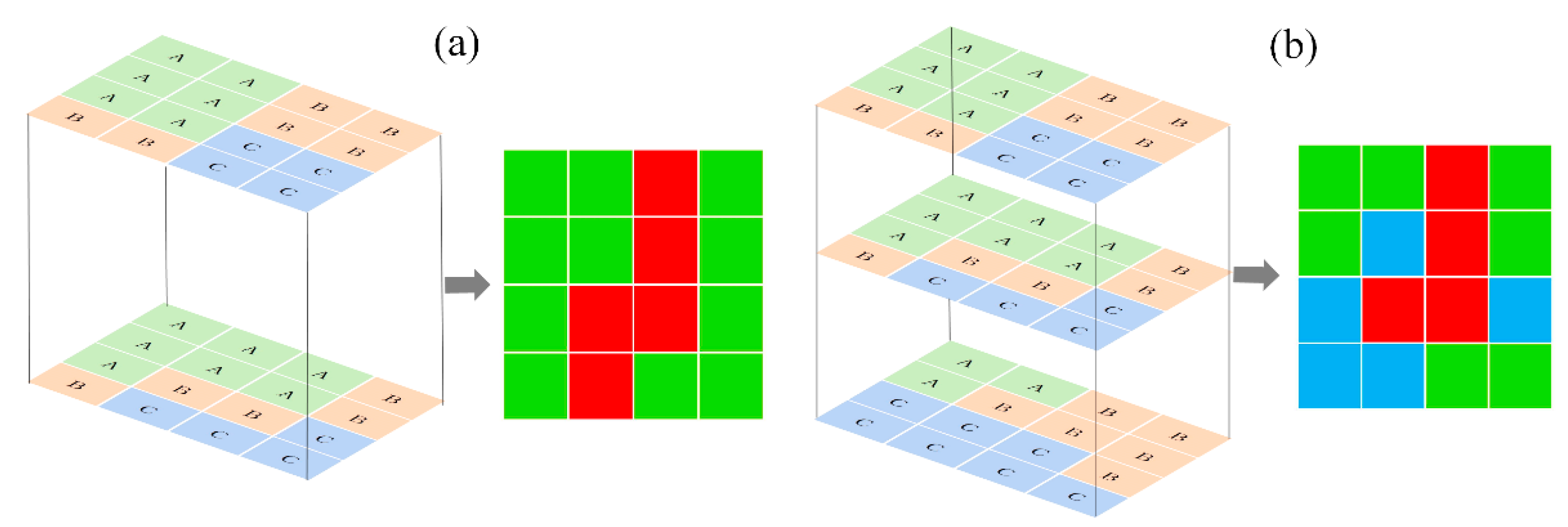
Figure 4.
The location of samples for nine LC types and sample sizes for each type are in the parentheses.
Figure 4.
The location of samples for nine LC types and sample sizes for each type are in the parentheses.
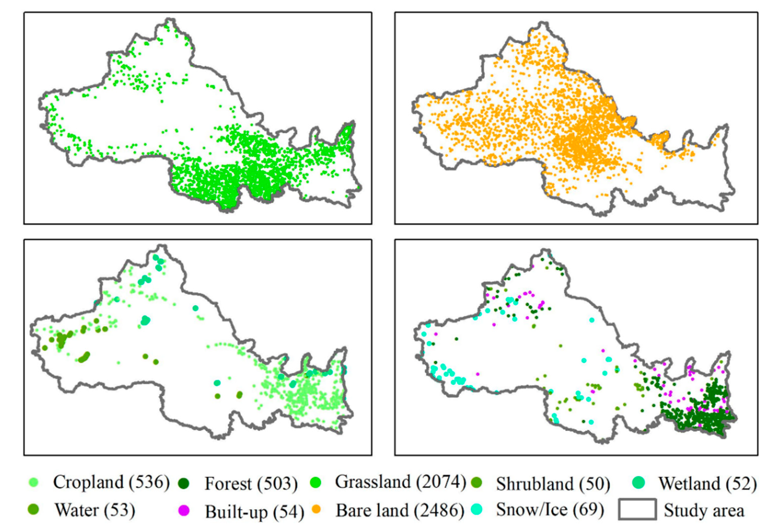
Figure 5.
The spatial (in)consistency of distribution of (a) three LC maps, (b) FROM vs. FCS, (c) FROM vs. Globe, and (d) FCS vs. Globe.
Figure 5.
The spatial (in)consistency of distribution of (a) three LC maps, (b) FROM vs. FCS, (c) FROM vs. Globe, and (d) FCS vs. Globe.

Figure 6.
Visual comparison between LC maps and Google Earth imagery for (a) completely correct, (b,c) basically correct, and (d) incorrect.
Figure 6.
Visual comparison between LC maps and Google Earth imagery for (a) completely correct, (b,c) basically correct, and (d) incorrect.


Table 1.
Main parameters of the three 30 m LC maps.
| LC Maps | First-Level LC Types | Time | Reported OA | Method | Satellite | Production Institution |
|---|---|---|---|---|---|---|
| FROM | 10 | 2017 | 72.76% | Random Forest | Landsat TM/ETM+/OLI | Tsinghua University |
| Globe | 10 | 2020 | 80.3% | POK (pixels, objects, knowledge) | Landsat TM/ETM+, HJ-1 A/B, GF-1 | National Geomatics Center of China |
| FCS | 9 | 2020 | 81.4% | Local random forest | Landsat TM/ETM+/OLI, Sentinel-1 SAR | Chinese Academy of science |
Table 2.
The grouped classification scheme and its response to the original classification schemes.
| Merged Type | Code | FROM | Code of FROM | Globe | Code of Globe | FCS | Code of FCS | Legend RGB Values |
|---|---|---|---|---|---|---|---|---|
| Cropland | 1 | Cropland | 10 | Cropland | 10 | Cropland | 10, 11, 12, 20 | 162, 255, 115 |
| Forest | 2 | Forest | 20 | Forest | 20 | Forest | 50, 60, 61, 62, 70, 71, 72, 80, 81, 82, 90 | 38, 115, 0 |
| Grassland | 3 | Grassland | 30 | Grassland | 30 | Grassland | 130 | 76, 230, 0 |
| Shrubland | 4 | Shrubland Tundra | 40 70 | Shrubl and Tundra | 40 70 | Shrubland | 120, 121, 122 | 112,168,0 |
| Wetland | 5 | Wetland | 50 | Wetland | 50 | Wetlands | 180 | 0, 220, 130 |
| Water | 6 | Water | 60 | Water | 60 | Waterbody | 210 | 0, 92, 255 |
| Built-up | 7 | Built-up | 80 | Impervious surfaces | 80 | Impervious surfaces | 190 | 197, 0, 255 |
| Bare land | 8 | Bare land | 90 | Bare land | 90 | Bare areas | 140, 150, 152, 153, 200, 201, 202 | 255, 170, 0 |
| Permanent Snow/Ice | 9 | Snow/Ice | 100 | Snow/Ice | 100 | Permanent ice and snow | 220 | 0, 255, 197 |
Table 3.
The area of nine classes of the three LC products (unit: km2).
| Classes | Code | FROM | Percentage in FROM | FCS | Percentage in FCS | Globe | Percentage in Globe | Mean | Percentage in Mean |
|---|---|---|---|---|---|---|---|---|---|
| Cropland | 1 | 216,212.68 | 7.02% | 261,122.23 | 8.47% | 287,936.88 | 9.34% | 255,090.60 | 8.28% |
| Forest | 2 | 181,001.87 | 5.87% | 204,152.61 | 6.63% | 171,546.38 | 5.57% | 185,566.96 | 6.02% |
| Grassland | 3 | 747,045.07 | 24.24% | 953,984.49 | 30.96% | 968,644.33 | 31.43% | 889,891.30 | 28.88% |
| Shrubland | 4 | 82,94.93 | 0.27% | 57,296.97 | 1.86% | 25,127.08 | 0.82% | 30,239.66 | 0.98% |
| Wetland | 5 | 6733.39 | 0.22% | 8236.69 | 0.27% | 15,379.13 | 0.50% | 10,116.41 | 0.33% |
| Water | 6 | 41,828.73 | 1.36% | 29,426.57 | 0.95% | 33,459.26 | 1.09% | 34,904.85 | 1.13% |
| Built-up | 7 | 28,424.48 | 0.92% | 19,117.23 | 0.62% | 26,492.52 | 0.86% | 24,678.08 | 0.80% |
| Bare land | 8 | 1,800,097.44 | 58.42% | 1,481,606.52 | 48.08% | 1,502,246.16 | 48.75% | 1,594,650.04 | 51.74% |
| Permanent Snow/Ice | 9 | 51,870.21 | 1.68% | 66,525.08 | 2.16% | 51,768.55 | 1.68% | 56,721.28 | 1.84% |
Table 4.
Overall similarity coefficient (OS) (%) and individual class similarity (CS) (%) coefficient among different maps.
Table 4.
Overall similarity coefficient (OS) (%) and individual class similarity (CS) (%) coefficient among different maps.
| LC Maps | OS | CScrop | CSForest | CSGrassland | CSShrubland | CSWetland | CSWater | CSBuilt-up | CSBareland | CSsnow/ice |
|---|---|---|---|---|---|---|---|---|---|---|
| Three Maps | 65.96% | 60.49% | 69.94% | 52.02% | 0.26% | 2.05% | 69.68% | 19.95% | 76.93% | 52.05% |
| FROM vs. FCS | 76.29% | 73.97% | 82.12% | 65.21% | 6.96% | 6.87% | 72.81% | 26.96% | 84.65% | 63.28% |
| FROM vs. Globe | 76.95% | 69.74% | 77.77% | 66.34% | 1.27% | 8.45% | 70.43% | 24.16% | 86.15% | 63.48% |
| FCS vs. Globe | 75.23% | 71.37% | 74.00% | 68.77% | 2.01% | 7.57% | 80.09% | 49.15% | 83.81% | 57.65% |
Table 5.
Accuracy measures were derived from confusion matrices of three LC maps.
| Products | FROM | FCS | Globe | |||
|---|---|---|---|---|---|---|
| Classes | PA | UA | PA | UA | PA | UA |
| Cropland | 74.07% | 86.68% | 89.74% | 87.45% | 88.62% | 78.64% |
| Forest | 92.05% | 91.14% | 91.25% | 92.47% | 79.72% | 87.36% |
| Grassland | 70.78% | 87.43% | 79.94% | 93.82% | 83.12% | 84.63% |
| Shrubland | 64.00% | 91.43% | 84.00% | 66.22% | 64.00% | 62.75% |
| Wetland | 55.77% | 80.56% | 80.77% | 85.71% | 94.23% | 73.13% |
| Water | 98.11% | 80% | 96.23% | 94.64% | 90.57% | 87.27% |
| Built-up | 64.62% | 56.76% | 83.08% | 90.00% | 86.15% | 70.89% |
| Bare land | 96.89% | 80.25% | 91.99% | 97.66% | 89.32% | 89.91% |
| Permanent Snow/Ice | 72.41% | 77.78% | 91.38% | 94.83% | 65.52% | 70.37% |
| OA | 83.49% | 87.07% | 85.69% | |||
| Kappa | 0.757 | 0.824 | 0.793 | |||
Disclaimer/Publisher’s Note: The statements, opinions and data contained in all publications are solely those of the individual author(s) and contributor(s) and not of MDPI and/or the editor(s). MDPI and/or the editor(s) disclaim responsibility for any injury to people or property resulting from any ideas, methods, instructions or products referred to in the content. |
© 2022 by the authors. Licensee MDPI, Basel, Switzerland. This article is an open access article distributed under the terms and conditions of the Creative Commons Attribution (CC BY) license (https://creativecommons.org/licenses/by/4.0/).
Share and Cite
MDPI and ACS Style
Bie, Q.; Shi, Y.; Li, X.; Wang, Y. Contrastive Analysis and Accuracy Assessment of Three Global 30 m Land Cover Maps Circa 2020 in Arid Land. Sustainability 2023, 15, 741. https://doi.org/10.3390/su15010741
AMA Style
Bie Q, Shi Y, Li X, Wang Y. Contrastive Analysis and Accuracy Assessment of Three Global 30 m Land Cover Maps Circa 2020 in Arid Land. Sustainability. 2023; 15(1):741. https://doi.org/10.3390/su15010741
Chicago/Turabian StyleBie, Qiang, Ying Shi, Xinzhang Li, and Yueju Wang. 2023. "Contrastive Analysis and Accuracy Assessment of Three Global 30 m Land Cover Maps Circa 2020 in Arid Land" Sustainability 15, no. 1: 741. https://doi.org/10.3390/su15010741
Note that from the first issue of 2016, this journal uses article numbers instead of page numbers. See further details here.