Quantitative Analysis and Correction of Temperature Effects on Fluorescent Tracer Concentration Measurement

1
College of Agriculture and Food, Kunming University of Science and Technology, Kunming 650500, China
2
USDA-ARS Application Technology Research Unit, Wooster, OH 44691, USA
3
Department of Agricultural Engineering and Technology, Ege University, 35040 Izmir, Turkey
*
Author to whom correspondence should be addressed.
Sustainability 2020, 12(11), 4501; https://doi.org/10.3390/su12114501
Submission received: 20 March 2020
/
Revised: 26 May 2020
/
Accepted: 27 May 2020
/
Published: 2 June 2020
(This article belongs to the Special Issue Precision Agriculture and Sustainability)
Abstract
:To ensure an accurate evaluation of pesticide spray application efficiency and pesticide mixture uniformity, reliable and accurate measurements of fluorescence concentrations in spray solutions are critical. The objectives of this research were to examine the effects of solution temperature on measured concentrations of fluorescent tracers as the simulated pesticides and to develop models to correct the deviation of measurements caused by temperature variations. Fluorescent tracers (Brilliant Sulfaflavine (BSF), Eosin, Fluorescein sodium salt) were selected for tests with the solution temperatures ranging from 10.0 °C to 45.0 °C. The results showed that the measured concentrations of BSF decreased as the solution temperature increased, and the decrement rate was high at the beginning and then slowed down and tended to become constant. In contrast, the concentrations of Eosin decreased slowly at the beginning and then noticeably increased as temperatures increased. On the other hand, the concentrations of Fluorescein sodium salt had little variations with its solution temperature. To ensure the measurement accuracy, correction models were developed using the response surface methodology to numerically correct the measured concentration errors due to variations with the solution temperature. Corrected concentrations using the models agreed well with the actual concentrations, and the overall relative errors were reduced from 42.36% to 2.91% for BSF, 11.72% to 1.55% for Eosin, and 2.68% to 1.17% for Fluorescein sodium salt. Thus, this approach can be used to improve pesticide sprayer performances by accurately quantifying droplet deposits on target crops and off-target areas.
1. Introduction
Applications of pesticide have ensured a noticeable increase in crop yields and high-quality food production [1,2,3,4]. However, excessive pesticide use due to improper spray applications has caused great concerns on risks to health and damage to the environment and sensitive ecosystems.
To reduce pesticide waste, the performances of agricultural sprayers need to be evaluated adequately and accurately [5,6]. Fluorescent tracers have been widely used to simulate pesticides in field tests, including the determination of pesticide spray distribution, deposition, and drift [7,8,9,10,11,12,13,14,15], and the assistance of sprayer design and improvement [16,17,18,19,20]. This is because fluorescent tracers are relatively highly sensitive, economical, practical, and non-poisonous compared to the analysis of active ingredients in pesticides [21,22,23,24]. During the field spray tests, fluorescent tracer is usually mixed in water first, and then the spray solution is discharged as spray droplets in a cloud to the plants. Some droplets deposit in the target area while some reach the ground or drift in the air. Collecting spray samples from target and off-target areas and quantifying the fluorescent tracers on the samples can help determine sprayer performances. The quantification of fluorescent tracers is processed by washing tracers off the samples with a given amount of distilled water, and then using a fluorometer to measure the fluorescent concentration in the washed solution. Because the fluorescent tracer concentration in the spray solution is a pre-determined constant, the amount of spray deposits on the samples can be calculated from the amount of fluorescent tracers measured.
For techniques associated with injection spray, the mixing of pesticide and diluent in the line to the nozzles should be adequate to make sure mixtures are uniform. Hence, quantifying mixing uniformity has been identified as an important subject for evaluating sprayer injection systems [25,26,27]. One effective method for performance evaluation utilizes fluorescent tracers which are injected into the carrier stream. The resulting concentrations of mixture are then estimated based on fluorescent analysis by fluorometers [28,29].
However, there are rising concerns about the measurement accuracy due to the stability of fluorescence during experiments. Various factors can cause a severe inaccuracy of fluorescence analysis. Considerable investigations have been reported on degradation by solar radiation and photodegradation of commonly used fluorescent tracers, which can result in a severe deviation of the test results [30,31,32]. The fluorescent strength of some fluorescent tracers behaved differently in alkaline or acidic solutions. For example, the fluorescence of Brilliant Sulfaflavine (BSF) and Eosin remained nearly constant over the solution pH range of 6.9–10.4; however, Fluorescein had much higher fluorescent sensitivity than BSF and Eosin [33,34]. The variation of solution temperature is another critical factor that can influence fluorescent measurement accuracy. For this reason, some fluorometer manufacturers suggest to keep solutions at stable ambient temperatures, but little information is available on how the temperature can affect fluorometer measurements. For example, Trilogy Laboratory Fluorometer specifies that the operating temperature for its fluorometer should be kept in the range of 15–40 °C, and recalibration is needed if the ambient temperature changes by ±10 °C [35]. In an actual experimental scenario, it is found that the effects of temperature on the deviation of fluorescent analysis varies with the type of fluorescent substances. For some types of fluorescent tracers, temperature effects on the concentration measurement have been underestimated. Taking BSF as an example, a slight variation in the solution temperature can lead to significant measurement errors by a fluorometer. However, there are few reports available about the effect of temperature on the measured concentration of fluorescent tracers commonly used in the evaluation of pesticide spray application efficiency and spray mixture uniformity.
Evaluating the effects of temperature on the measurement accuracy of fluorescent tracers is of importance, because it is difficult to maintain a constant solution temperature under certain analytical conditions. For example, some tests must be conducted with field in-situ measurements of spray deposition. For the field tests, the instruments generally operate in a wide range of outdoor temperatures, and the solution temperature also varies with the environment. Similarly, for indoor laboratory experiments, samples for measurements also have the temperature variation problem, which can be significantly lower or higher than the desired temperature. Therefore, the influence of the variation of temperature on the accuracy of fluorescent tracer analysis should be determined before and after the tests.
Furthermore, it is not only important to know the temperature dependence of the fluorescent tracers, but also to propose a method that can increase the accuracy of fluorescent tracer measurements. The behaviors of florescent tracers under various temperatures are predictable, and they have been generally used for thermometry purposes, such as non-contact measurement of fluid temperature at the microscale with high accuracy [36,37,38,39,40,41]. Therefore, it is also possible to develop reliable correction models [42] which can be used to compensate the deviation of measurement results caused by the solution’s temperature. Response surface analysis is a set of mathematical techniques. By graphing the results of polynomial regression analyses in a three-dimensional space, response surface analysis can provide relationships between predictor variables and an outcome variable [43,44]. In this study, response surface methodology was adopted to establish the relationship among measured concentration, temperature, and nominal concentration to correct the measurement errors.
The objectives of this research were to examine the effect of the changes of solution temperatures on the measured concentrations of fluorescent tracers, and to develop models to compensate the deviation of measurement results caused by temperature changes. The effort of this research was to minimize analytical errors in the concentration measurement of fluorescent tracers, in order to increase the accuracy of accessing pesticide spray mixture uniformity and quantifying spray deposition and drift.
2. Materials and Methods
2.1. Fluorescent Tracers Used
Three typical fluorescent tracers were selected for the tests: BSF (MP Biomedicals, Inc., Aurora, OH, USA), Eosin (Acros Organics, Thermo Fisher Scientific, Pittsburgh, PA, USA), and Fluorescein sodium salt (Sigma-Aldrich, Inc., Saint Louis, MO, USA). BSF and Eosin were the yellowish free acid dyes. Fluorescein sodium salt contained 70% dye content and 30% sodium salt. The excitation and emission wavelengths, Chemical Abstracts Service (CAS) registry number, molecular weight, chemical formula, and fluorescence quantum yield of these tracers, indicated by the manufacturers, are listed in Table 1.
2.2. Fluorescent Tracer Solutions
Pilot work is necessary to identify the linear range for each type of tested fluorescent tracers. In this study, the linear range for each tested fluorescent tracer was identified by preparing sample solutions at different concentrations. Then, linearity was checked by measuring sample solutions from minimum detectable concentrations. If the sample was still in the linear range, the reading would increase in direct proportion to the concentration. If the reading did not increase in direct proportion to the concentration, or if the reading decreased instead, this meant “signal quenching” had begun and the sample was beyond the linear range of the fluorophore. The pilot work of this study identified that the linear range was between 5.00 and 30.00 mg L−1 for BSF, 37.50 and 600.00 µg L−1 for Eosin, and 4.88 and 156.25 µg L−1 for Fluorescein sodium salt.
For each type of tested fluorescent tracer and at each concentration, initial solutions were prepared and then diluted to the desired concentrations. A digital scale with readability to 0.01 g was used to weigh each tracer. A graduated cylinder class with 1.0 mL subdivision and ±0.5 mL tolerance was used to measure the volume of purified distilled water. The concentrations of tracers in the solutions were 5.00, 10.00, 15.00, 20.00, 25.00, and 30.00 mg L−1 for BSF, 37.50, 75.00, 150.00, 300.00, and 600.00 µg L−1 for Eosin, and 4.88, 9.77, 19.53, 39.06, 78.12, and 156.25 µg L−1 for Fluorescein sodium salt, respectively. For each concentration, five samples were prepared for five replications and each sample was stored in a 3.5 mL transparent cuvette.
2.3. Solution Temperatures
Fluorescence intensities were measured with a portable fluorometer (Turner Designs, Inc., San Jose, CA, USA). This fluorometer used fluorescence optical modules which contained the necessary light source and pre-set filters for the required application. The tests were conducted with the fluorometer located inside a laboratory with a constant ambient temperature. The laboratory was equipped with an automatic controller and a Circular Chart Recorder (model: DR5000, Future Design Controls, Inc., Bridgeview, IL, USA) to control the ambient temperature continuously. During the measurement, if the cuvette was kept inside the fluorometer for too long, the fluorometer could raise the solution temperature significantly. Therefore, cuvettes that contained solution samples were inserted into the fluorometer for only about 6 s. Within the 6 s time duration, the increase of solution temperature was less than 0.3 °C.
Before each test, a digital scale (model: Practum1102-1S, Sartorius, Goettingen, Germany) with readability to 0.01 g was used to weight each tracer. The ratio between the fluorescent tracer weight and the distilled water volume was determined to represent the actual concentration or nominal concentration of the solution.
All tests were conducted with the ambient temperature ranging from 19.0 °C to 21.0 °C. As shown in Figure 1, temperatures of tracer solution samples were adjusted with the following step for analysis. The fluorometer cuvettes containing fluorescent tracer solution samples were submerged into the water bath container. Cold water and warm water were alternatively applied to adjust the temperature until the desired value was reached. A stirring rod was used to speed up heat exchange and temperature uniformity distribution. Probe digital thermometers (PDT650, UEi Test Instruments, Beaverton, OR, USA) were used to monitor the tracer solution temperatures in the cuvettes and the water temperature in the container consistently. The samples were kept in the container for at least 10 min, for the temperature reading of the thermometer placed in the cuvette to reach an interval of ±0.5 °C of the desired temperature.
Since the tests in this study were conducted in an indoor laboratory, the factor of photodegradation caused by solar exposure was excluded. To avoid other potential sources of degradation, for each type of fluorescent tracer and under each concentration condition, the time elapsed between the sample preparation and measurement were 4 h. This interval was used for weighing the tracers, mixing with distilled water, diluting, adjusting the temperature, and measuring with the fluorometer. Within such a short time duration, readings were stable. Moreover, the measurements of fluorescent intensity in this study have been based on the assumption that for the same concentration of fluorescent tracer solution with the same temperature and same pH value, readings from the same fluorometer should be constant. the pH value of the purified distilled water used in this study was 6.4. To avoid solution samples contacting with the ambient air containing CO2 and to keep the solution pH condition consistent, the cuvettes containing solution samples were sealed with air-tightened caps. After the solution samples in the cuvettes were sealed with air-tightened caps, their pH value could be kept constant. To avoid contaminations caused by opening and closing the cuvettes filled with fluorescent tracer solutions, five additional cuvettes filled only with distilled water were used to verify the solution temperatures. The five cuvettes were randomly distributed inside the water container. The temperatures in these five cuvettes were measured within the error range of 0.5 °C.
In this study, solution temperatures of 10.0 to 45.0 °C with 5.0 °C intervals were selected. The fluorometer manufacturer recommended that the ambient temperature should be within 15.0–40.0 °C during operation [35]. For some tests, the solution temperature could be higher or lower than the ambient temperature. Therefore, temperatures with ±5.0 °C above and below the fluorometer manufacturer’s recommended temperature range (10.0 and 45.0 °C) were used along with the recommended range.
2.4. Model Development
Response surface methodology was used to establish the relationships between the measured concentration, temperature, and corrected concentration. A statistical analysis and polynomial regression with response surface analysis was performed using the function Curve Fitting Toolbox™ in the Matlab software (ver. 8.5.1.281278 (R 2015a) Service Pack 1, MathWorks, Inc., Natick, MA, USA). The Curve Fitting application was used to fit response surfaces to fluorometer data to determine the effects of temperature on the measured concentrations.
In the response to the surface analysis approach, a polynomial regression with the third order functions was processed. This model was used for prediction of the corrected concentrations. The Fitting Tool was applied and the individual model could be interpreted as a surface fitting function of the experimental data.
The general form of a complete third-degree polynomial regression model in two variables (x, y) was expressed as:
where p00, p10, p01, p20, p11, p02, p30, p21, p12, and p03 are constants, x represents the solution temperature, and y represents measured concentration.
The constants of the equation were determined by the least square method. After fitting the models, surfaces and contour plots were constructed to predict the relationship between the independent variables and determine coefficient R2. R2 measured the successful level of the fit in explaining the variation of the data. An R2 closer to 1 indicated that a greater proportion of variance was accounted by the model and a better fitting result was reached. The residuals were the differences between the calculated and experimental results for a determined set of conditions. A satisfactory mathematical model fitted to experimental data must present low residual values. Therefore, residual plots of the fitted models were also constructed.
3. Results
3.1. Linear Range and Calibration Model
The fluorescent tracer calibration curves in Figure 2 were obtained with an ambient temperature ranging from 19.0 °C to 21.0 °C. The same ambient temperature range was used for establishing the correction model. The temperature of the solution samples in the cuvette for calibration was 20.0 ± 0.5 °C.
In order to achieve a fluorescent intensity that fell within the range of the fluorometer used, fluorescent tests were limited to the linear range of the response. As shown in Figure 2a–c, the linear range of concentrations used in this study was 5.00 to 30.00 mg L−1 for BSF, 37.50 to 600.00 μg L−1 for Eosin, and 4.88 to 156.25 μg L−1 for Fluorescein sodium salt, respectively.
The tracer concentration of the solution as a function of fluorescence intensity was calibrated before the tests. The calibration equation for the tracer concentration and fluorescence intensity was:
BSF tracer:
Eosin:
Fluorescein sodium salt:
where y is the tracer concentration in the solution and x is the fluorescence intensity.
3.2. Effect of Temperature on Measured Concentration of Fluorescent Tracers
3.2.1. Estimation of the Accuracy of the Fluorometer
Because random errors could be caused by tiny fluctuations in temperatures due to sample-to-sample variations—for example, because of temperature variations in the laboratory environment, the solution samples or the fluorometer itself—measuring the solution sample even with the same concentration by a fluorometer could result in slightly different readings each time. These errors could be reduced by taking the average of repeated measurements. To compare the fluorometer uncertainty regarding the observed sample-to-sample variations, overall average values for the coefficient of variation (CV) under tested nominal concentrations were calculated. For BSF with nominal concentrations ranging from 5.00 to 30.00 mg L−1, the overall average CV values were 1.01%, 0.97%, 1.16%, 1.29%, 1.66%, and 1.51%; for Eosin with nominal concentrations ranging from 37.50 to 600.00 µg L−1, the overall average CV values were 3.54%, 1.70%, 1.50%, 0.88%, and 0.74%; for Fluorescein sodium salt with nominal concentrations ranging from 4.88 to 156.25 µg L−1, the overall average CV values were 7.82%, 3.33%, 1.08%, 1.34%, 1.48%, and 0.69%, respectively. It was found that BSF had a slightly higher fluorometer measurement uncertainty at higher nominal concentrations. Conversely, Eosin and Fluorescein Sodium Salt had higher fluorometer uncertainty at lower concentrations.
3.2.2. BSF
Figure 3 shows the measured concentration of BSF solution with the variation of temperature from 10.0 to 45.0 °C. The measured concentration was obviously affected by the solution’s temperature. It was found that the measured concentration decreased as the solution temperature increased at all nominal concentrations. As the temperature was increased from 10.0 to 35.0 °C, a sharp drop in the measured concentration occurred over this temperature range. As the temperature increased further, the decrease rate slowed down, and the measured concentration tended to be consistent and stable. For example, at a nominal concentration of 20 mg L−1, the measured concentration was 36.41, 26.59, 20.45, 15.90, 12.83, 10.61, 8.92, and 7.78 mg L−1 when the solution temperature was 10.0, 15.0, 20.0, 25.0, 30.0, 35.0, 40.0, and 45.0 °C, respectively.
BSF should be considered as highly sensitive to temperatures, because a slight variation in solution temperatures could lead to a significant measurement error by the fluorometer. For instance, for the BSF solution of 30.00 mg L−1, the measured concentration decreased over 2.5 times (from 75.40 to 29.90 mg L−1) when the solution temperature increased from 10.0 to 20.0 °C.
For different nominal concentrations, the measured concentrations did not display a constant decrease trend with increased solution temperatures. As the temperature increased, the decrease of measured concentrations was found to be even more remarkable for samples with higher nominal concentrations. For example, at a nominal concentration of 5.00 mg L−1, the measured concentration was 7.65, 6.02, 4.95, 4.18, 3.50, 3.04, 2.66, and 2.37 mg L−1 when the solution temperature was 10.0, 15.0, 20.0, 25.0, 30.0, 35.0, 40.0, and 45.0 °C, respectively; however, at a nominal concentration of 30.00 mg L-1, the measured concentration was 75.44, 43.57, 29.88, 22.62, 17.61, 14.56, 11.90, and 9.92 mg L−1.
These results revealed that relatively higher nominal concentrations could aggravate a negative influence of the solution temperature on the measured concentrations and could reduce the detection accuracy. For the BSF solution, over the temperatures tested (10.0 to 45.0 °C), the relative error of measured concentrations to nominal concentrations fell in the range of 1.04–53.08% (average 32.44%), 1.28–60.38% (average 35.83%), 0.93–72.59% (average 39.17%), 2.23–82.07% (average 42.14%), 0.66–120.84% (average 49.39%), and 0.39–151.46% (average 55.21%) for the nominal concentrations of 5.00, 10.00, 15.00, 20.00, 25.00, and 30.00 mg L−1, respectively.
Table 2 shows the mean measured concentration and CV of the BSF solutions across the eight temperatures at six different nominal concentrations. The CV increased from 42.44% to 78.18% as the nominal concentration increased from 5.00 to 30.00 mg L−1. The results of the statistical analysis also indicated that for all the nominal concentrations (5.00, 10.00, 15.00, 20.00, 25.00, and 30.00 mg L−1), the means of measured concentrations were significantly different (p < 0.01) for the BSF solution under tested solution temperature conditions (10.0, 15.0, 20.0, 25.0, 30.0, 35.0, 40.0, and 45.0 °C). The solution temperature influenced the measured concentrations more significantly when the measurement was conducted at relatively higher nominal concentrations.
3.2.3. Eosin
As with BSF, the measured concentration of Eosin was also affected by the solution’s temperature (Figure 4). However, the measured concentration of Eosin slightly decreased at first when the temperature increased from 10.0 °C to 15.0 °C or 20.0 °C, and then increased smoothly as the temperature increased further. Compared to BSF, the measured concentration of Eosin was more temperature-independent at lower temperatures, but was more influenced by higher temperatures. For example, at a nominal concentration of 150.00 μg L−1, the measured concentrations were 151.69, 149.49, 148.76, 156.25, 163.93, 171.08, 179.66, and 194.09 μg L−1 when the solution temperatures were 10.0, 15.0, 20.0, 25.0, 30.0, 35.0, 40.0, and 45.0 °C, respectively.
For the tested nominal concentrations, the influence of temperature on the measured concentrations was lowest at the nominal concentration of 150.00 μg L−1. Relatively lower or higher nominal concentrations were more severely influenced by temperature, and the measurement accuracy was lower. For the Eosin solution, over the tested temperature range from 10 to 45 °C, the relative error of measured concentrations to nominal concentrations fell in the range of 0.14–34.43% (average 13.71%), 0.20–32.82% (average 12.58%), 0.34–29.40% (average 9.87%), 0.49–31.46% (average 11.15%), and 0.43–30.64% (average 11.29%) for the nominal concentrations of 37.50, 75.00, 150.00, 300.00, and 600.00 μg L−1, respectively.
The mean measured concentrations were affected by the solution temperature at different nominal concentrations. The CV decreased first from 10.62 to 9.90%, and then increased to 11.41% as the nominal concentration increased from 37.50 to 600.00 μg L−1 (Table 2). The results of the statistical analysis indicated that the differences in the means of measured concentrations were significant (p < 0.01) for Eosin solutions under tested solution temperature conditions (10.0, 15.0, 20.0, 25.0, 30.0, 35.0, 40.0, and 45.0 °C).
3.2.4. Fluorescein Sodium Salt
Figure 5 shows the effect of temperature on the measured concentration of Fluorescein sodium salt. Differently from BSF and Eosin, the measured concentrations of Fluorescein sodium salt did not display a constant increase or decrease trend with increased or decreased solution temperatures. Instead, it fluctuated slightly with the temperatures tested. It was also found that among the three tracers the measured concentration of Fluorescein sodium salt was the least affected by solution temperature. For example, at a nominal concentration of 39.06 μg L−1, the measured concentrations were 38.45, 38.87, 38.70, 38.57, 39.85, 38.89, 38.13, and 39.22 μg L−1 when the solution temperatures were 10.0, 15.0, 20.0, 25.0, 30.0, 35.0, 40.0, and 45.0 °C, respectively. Especially, low nominal concentrations led to a nearly constant measured concentration over the tested temperature range. At a nominal concentration of 4.88 μg L−1, the measured concentrations were 4.70, 5.50, 5.54, 5.15, 4.64, 4.45, 4.69, and 5.65 μg L−1 when the solution temperatures were 10.0, 15.0, 20.0, 25.0, 30.0, 35.0, 40.0, and 45.0 °C, respectively.
The least affected tracer by the variation of temperature had the highest measurement accuracy. For the Fluorescein sodium salt solution, over the temperature range from 10.0 to 45.0 °C, the relative error of the measured concentrations to nominal concentrations fell in the range of 0.01 to 1.82% (with an average of 0.95%), 0.09 to 3.02% (with an average of 1.08%), 0 to 4.91% (with an average of 2.61%), 0.23 to 6.85% (with an average of 2.81%), 0.04 to 5.50% (with an average of 2.30%), and 0.02 to 5.27% (with an average of 3.01%) for nominal concentrations of 4.88, 9.77, 19.53, 39.06, 78.12, and 156.25 μg L−1, respectively.
The coefficients of variation for the mean concentrations across the five temperatures at six different nominal concentrations fluctuated slightly between 1.10% and 2.26%—much less than those of the BSF and Eosin solutions. It was noted that for the nominal concentrations of 4.88 and 9.77 μg L−1 there was no significant difference (p > 0.05) between the means of measured concentrations. Hence, for these two concentrations, the measured concentration could be considered as agreeing satisfactorily with the nominal concentration. However, for the nominal concentrations of 19.53, 39.06, 78.12, and 156.25 μg L−1, the differences between means of measured concentration were significant (p < 0.01) under tested solution temperature conditions (10.0, 15.0, 20.0, 25.0, 30.0, 35.0, 40.0, and 45.0 °C).
Thus, the measured concentrations were strongly affected by the temperature of the fluorescent tracer solutions, except for Fluorescein sodium salt. BSF was the most sensitive to temperature changes among the tested nominal concentrations, followed by Eosin.
3.3. Correction Models
The experimental results showed that the variation in measured concentration with temperature depended on the type of tested florescent tracers; therefore, a specific response surface model was developed for a specific fluorescent tracer.
The surface response model for BSF was
for Eosin, it was
and for Fluorescein sodium salt, it was
The R2 values for the three models were 0.9957 for BSF, 0.9997 for Eosin, and 0.9996 for Fluorescein sodium salt. A higher R2 indicated a more satisfactory adjustment of the cubic polynomial model to the experimental data and a higher correlation between the measured and the predicted values.
A three-dimensional visualization of the predicted models could be obtained by the response surface plots shown in Figure 6.
The residual graphs were plotted in Figure 7a–c. The low residuals indicated that the regression models for BSF, Eosin, and Fluorescein sodium salt tracers agreed well with the actual solution concentrations. Thus, the models were adequate to make precise interpretations about the behavior of fluorescent tracers under various solution temperatures.
With the correction model, the analytical errors of corrected concentration and nominal concentration were calculated and evaluated. The corrected concentrations for the BSF tracer are shown in Figure 8a. The relative error of corrected concentrations to nominal concentrations fell in the range of 0.03–25.93% (6.86% average), 0.88–3.24% (1.72% average), 0.46–5.28% (2.29% average), 0.15–6.82% (2.80% average), 0.06–2.54% (1.29% average), and 0.08–4.55% (2.50% average) for the nominal concentrations of 5.00, 10.00, 15.00, 20.00, 25.00, and 30.00 mg L−1, respectively.
The coefficients of variation for the mean corrected concentrations of the BSF solution across eight temperatures at six different nominal concentrations, based on Equation (5), increased greatly (Table 3) compared to the values in Table 2. The highest coefficients of variation were recorded as 10.21% at the nominal concentration of 5 mg L−1, while the rest were lower than 2.94%.
The corrected concentrations for Eosin are shown in Figure 8b. For the tested temperatures (10.0 to 45.0 °C), the relative error of corrected concentrations to nominal concentrations fell in the ranges of 0.63–4.93% (2.87% average), 0.10–4.43% (2.30% average), 0.34–2.23% (1.09% average), 0.04–1.52% (0.77% average), and 0.03–1.39% (0.73% average) for the nominal concentrations of 37.50, 75.00, 150.00, 300.00, and 600.00 μg L−1, respectively.
The coefficients of variation for the mean corrected concentrations of Eosin decreased from 3.51% to 0.88% as the nominal concentrations increased from 37.50 to 600.00 μg L−1 (Table 3).
For Fluorescein sodium salt (Figure 8c), the differences between corrected concentrations and nominal concentrations at different temperatures were very small and could be negligible. The coefficients of variation for mean corrected concentrations across eight temperatures at four nominal concentrations fluctuated between 1.54% and 2.26% (Table 3). Thus, it was unnecessary to apply the correction model for Fluorescein sodium salt.
For the tracers of BSF, Eosin, and Fluorescein sodium salt with solution temperatures ranging from 10.0 to 45.0 °C, the above analyses showed that the relationships among the measured concentration, temperature, and corrected concentration were well correlated. The low relative errors and coefficients of variation with the correction models indicated that the variations in measured concentrations caused by the solution temperatures could be corrected accurately.
4. Discussion
The measured concentration of different fluorescent tracers responded differently to their solution temperatures. To avoid this problem, pilot works should be essential to figure out the desired temperature range for different types of fluorescent tracers for ensuring the accurate measurement.
For laboratory tests, it is necessary to follow the fluorometer manufacturer’s recommendations and control the ambient temperature within a specific range to reduce the analytical errors. If the tests require high-precision measurements for certain types of fluorescent tracers, pilot tests are necessary to identify desired temperature ranges that could provide measurement results with acceptable accuracy. If the temperature cannot be adjusted to a desired range, the temperature should be recorded along with the measured concentration, and the correction models should then be applied to correct the measured concentrations.
For instruments that are deployed for in-situ field measurements, due to the difficulty of controlling the ambient temperature, stable tracers should be used. Otherwise, it is necessary to determine the relationship between the solution temperature and the tracer concentration prior to its use. To minimize analytical errors, the solution temperature should also be measured and recorded. After the experiments, correction models should be used to compensate the deviation of measured concentrations caused by the solution temperature.
It should be noted that fluorometer manufacturers usually suggest a recalibration when new fluorescent tracers are used. Therefore, when the fluorescent tracer changes to a different provider, manufacture, or batch number, a recalibration is necessary. Accordingly, to ensure measurement precision and accuracy, correction models also need to be re-established by using the method presented in this study. Although the specific equations of the correction models obtained in this study may not be directly applied by other researchers, the methodology presented in this study could be effectively generalized and applied by other researchers to numerically correct the measured concentration errors due to variations in the solution temperature.
This study also provided a technique for developing fluorometers equipped with a temperature compensation function. In this way, when the fluorometer measured the fluorescent intensity, the solution temperatures were also acquired at the same time to fit into the correction models. As a result, the error caused by the temperature variation could be compensated by using specific correction models embedded in the fluorometer for different tracers.
Actually, the true concentration was not changed throughout the experiment. This is because the amount of fluorescent tracers (solute) in distilled water (solvent) was unchanged. However, during the reading, the variation of the measured concentrations was caused by the effects of the changes in the solution temperature on the fluorescent strengths. It has been found that the influence of temperature on the evolution of the fluorescence quantum yield is explained by the competition between the radiative relaxation mechanisms (fluorescence, phosphorescence) and the non-radiative relaxation mechanisms (inter-system crossing, internal conversion) [45]. For the future research, physical reasons for the temperature effect on the tracer concentration should be discovered, considering the following aspects: investigating the mechanisms of temperature effects based on spectroscopy, establishing models for the spectra of the dyes (both emission and absorption) as a function of the temperature, and analyzing the absorption of the incident excitation and fluorescence re-absorption. Because the temperature dependence of Eosin and Fluorescein disodium is driven by two mechanisms that are very different, one has a dependence on the quantum yield and the other on the absorption cross section. This has an influence on the interpretation of the results and should be explored and discussed in the future research.
5. Conclusions
The effect of solution temperatures on the measured fluorescent concentration for fluorescent tracers of BSF, Eosin, and Fluorescein sodium salt was investigated. The following conclusions are highlighted.
The measured concentrations of BSF, Eosin, and Fluorescein sodium salt were influenced by the solution temperature and the effect varied with the type of the tracer. Among the three fluorescent tracers, BSF was the most affected by the solution temperature, followed by Eosin, while the influence on Fluorescein sodium salt was negligible.
The measured concentrations of BSF decreased as the solution temperature increased. The decrement rate was high at first, then slowed down, and then tended to become constant as the temperature increased. In contrast, the measured concentrations of Eosin decreased slowly at first and then increased noticeably as the temperatures increased.
Third-order polynomial correction models were developed to minimize the error in the fluorescent analysis. These models, using the response surface methodology, enabled numerical corrections of the measured concentration errors due to variations of the solution temperatures. The corrected concentrations agreed well with the nominal concentrations. The overall relative errors were reduced from 42.36% to 2.91% for BSF, 11.72% to 1.55% for Eosin, and 2.68% to 1.17% for Fluorescein sodium salt.
Therefore, the accuracy of the fluorescent concentration measurements should be examined with the solution temperatures to minimize analysis errors during the fluorescent tracer selection, for accurate quantifications of spray deposition on targets and off-target losses, and for obtaining spray mixture uniformity. It was necessary to adjust the fluorescent tracer solution temperature to a specific desired range for sample analyses. If the solution temperature adjustment is not feasible, the temperature should be recorded for each concentration measurement, and then the correction models should be applied to avoid measurement errors.
As a result of this research, it is recommended that spray sample analyses use the correction models if the analyses must be processed in the field; otherwise, the samples should be calibrated and analyzed in laboratories with the same constant ambient temperature.
Author Contributions
Conceptualization, Z.Z., H.Z. and H.G.; methodology, Z.Z.; software, Z.Z.; validation, Z.Z., H.Z., and H.G.; investigation, Z.Z.; resources, H.Z.; data curation, Z.Z.; writing—original draft preparation, Z.Z.; writing—review and editing, H.G. and H.Z.; visualization, Z.Z.; supervision, H.Z.; project administration, H.Z.; funding acquisition, H.Z. All authors have read and agreed to the published version of the manuscript.
Funding
This research was funded by the USDA-NIFA Specialty Crop Research Initiative, grant number 2015-51181-24253.
Acknowledgments
The authors gratefully acknowledge Adam Clark, Barry Nudd, and Andy Doklovic for setting up the experimental instrumentations. Mention of company or trade names is for description only and does not imply endorsement by the USDA. The USDA is an equal opportunity provider and employer.
Conflicts of Interest
The authors declare no conflict of interest.
References
- Carvalho, F.D.P. Agriculture, pesticides, food security and food safety. Environ. Sci. Policy 2006, 9, 685–692. [Google Scholar] [CrossRef]
- Cooper, J.; Dobson, H. The benefits of pesticides to mankind and the environment. Crop. Prot. 2007, 26, 1337–1348. [Google Scholar] [CrossRef]
- Popp, J.; Pető, K.; Nagy, J. Pesticide productivity and food security. A review. Agron. Sustain. Dev. 2012, 33, 243–255. [Google Scholar] [CrossRef]
- Gil, E.; Arnó, J.; Llorens, J.; Sanz, R.; Llop, J.; Rosell-Polo, J.R.; Gallart, M.; Escola, A. Advanced Technologies for the Improvement of Spray Application Techniques in Spanish Viticulture: An Overview. Sensors 2014, 14, 691–708. [Google Scholar] [CrossRef] [PubMed] [Green Version]
- Pascuzzi, S. Outcomes on the Spray Profiles Produced by the Feasible Adjustments of Commonly Used Sprayers in “Tendone” Vineyards of Apulia (Southern Italy). Sustainability 2016, 8, 1307. [Google Scholar] [CrossRef] [Green Version]
- Bochniak, A.; Kluza, P.A.; Kuna-Broniowska, I.; Koszel, M. Application of Non-Parametric Bootstrap Confidence Intervals for Evaluation of the Expected Value of the Droplet Stain Diameter Following the Spraying Process. Sustainability 2019, 11, 7037. [Google Scholar] [CrossRef] [Green Version]
- Grella, M.; Gallart, M.; Marucco, P.; Balsari, P.; Gil, E. Ground Deposition and Airborne Spray Drift Assessment in Vineyard and Orchard: The Influence of Environmental Variables and Sprayer Settings. Sustainability 2017, 9, 728. [Google Scholar] [CrossRef] [Green Version]
- Qin, W.-C.; Xue, X.; Zhou, Q.; Cai, C.; Wang, B.-K.; Jin, Y.-K. Use of RhB and BSF as fluorescent tracers for determining pesticide spray distribution. Anal. Methods 2018, 10, 4073–4078. [Google Scholar] [CrossRef]
- Vieira, B.C.; Butts, T.R.; Rodrigues, A.O.; Golus, J.A.; Schroeder, K.; Kruger, G.R. Spray particle drift mitigation using field corn (Zea mays L.) as a drift barrier. Pest Manag. Sci. 2018, 74, 2038–2046. [Google Scholar] [CrossRef]
- Bueno, M.R.; da Cunha, J.P.A.R.; de Santana, D.G. Assessment of spray drift from pesticide applications in soybean crops. Biosyst. Eng. 2017, 154, 35–45. [Google Scholar] [CrossRef]
- Wang, G.; Lan, Y.; Yuan, H.; Qi, H.; Chen, P.; Ouyang, F.; Han, Y. Comparison of Spray Deposition, Control Efficacy on Wheat Aphids and Working Efficiency in the Wheat Field of the Unmanned Aerial Vehicle with Boom Sprayer and Two Conventional Knapsack Sprayers. Appl. Sci. 2019, 9, 218. [Google Scholar] [CrossRef] [Green Version]
- Wang, C.; He, X.; Wang, X.; Wang, Z.; Wang, S.; Li, L.; Bonds, J.; Herbst, A.; Wang, Z. Testing method and distribution characteristics of spatial pesticide spraying deposition quality balance for unmanned aerial vehicle. Int. J. Agric. Boil. Eng. 2018, 11, 18–26. [Google Scholar] [CrossRef] [Green Version]
- Llop, J.; Gil, E.; Gallart, M.; Contador, F.; Ercilla, M. Spray distribution evaluation of different settings of a hand-held-trolley sprayer used in greenhouse tomato crops. Pest Manag. Sci. 2015, 72, 505–516. [Google Scholar] [CrossRef] [PubMed]
- Nairn, J.J.; Forster, W.A. Due diligence required to quantify and visualise agrichemical spray deposits using dye tracers. Crop. Prot. 2019, 115, 92–98. [Google Scholar] [CrossRef]
- O’Donnell, C.; Hewitt, A.; Dorr, G.; Ferguson, C.; Ledebuhr, M.; Furness, G.; Roten, R. Spraying: Evaluating spray drift and canopy coverage for three types of vineyard sprayers. Wine Viticul. J. 2017, 32, 42. [Google Scholar]
- di Prinzio, A.; Behmer, S.; Magdalena, J.; Chersicla, G. Effect of Pressure on the Quality of Pesticide Application in Orchards. Chil. J. Agric. Res. 2010, 70, 674–678. [Google Scholar] [CrossRef] [Green Version]
- Chen, Y.; Ozkan, H.E.; Zhu, H.; Derksen, R.C.; Krause, C. Spray deposition inside tree canopies from a newly developed variable-rate air-assisted sprayer. Trans. ASABE 2013, 56, 1263–1272. [Google Scholar]
- Felsot, A.S.; Unsworth, J.; Linders, J.; Roberts, G.; Rautman, D.; Harris, C.; Carazo, E. Agrochemical spray drift; assessment and mitigation—A review. J. Environ. Sci. Heal. Part B 2010, 46, 1–23. [Google Scholar] [CrossRef]
- Hoffmann, W.; Farooq, M.; Walker, T.; Fritz, B.; Szumlas, D.; Quinn, B.; Bernier, U.; Hogsette, J.; Lan, Y.; Huang, Y.; et al. Canopy Penetration and Deposition of Barrier Sprays from Electrostatic and Conventional Sprayers1. J. Am. Mosq. Control. Assoc. 2009, 25, 323–331. [Google Scholar] [CrossRef]
- Zhu, H.; Liu, H.; Shen, Y.; Liu, H.; Zondag, R. Spray deposition inside multiple-row nursery trees with a laser-guided sprayer. J. Env. Hortic. 2017, 35, 13–23. [Google Scholar]
- Arvidsson, T.; Bergström, L.; Kreuger, J. Spray drift as influenced by meteorological and technical factors. Pest Manag. Sci. 2011, 67, 586–598. [Google Scholar] [CrossRef] [PubMed]
- Lebeau, F.; Verstraete, A.; Stainier, C.; Destain, M. RTDrift: A real time model for estimating spray drift from ground applications. Comput. Electron. Agric. 2011, 77, 161–174. [Google Scholar] [CrossRef]
- Arvidsson, T.; Bergström, L.; Kreuger, J. Comparison of collectors of airborne spray drift. Experiments in a wind tunnel and field measurements. Pest Manag. Sci. 2011, 67, 725–733. [Google Scholar] [CrossRef] [PubMed]
- Xue, X.; Tu, K.; Qin, W.; Lan, Y.; Zhang, H. Drift and deposition of ultra-low altitude and low volume application in paddy field. Int. J. Agric. Biol. Eng. 2014, 7, 23–28. [Google Scholar]
- Zhu, H.; Ozkan, H.E.; Fox, R.D.; Brazee, R.D.; Derksen, R.C. Mixture uniformity in supply lines and spray patterns of a laboratory injection sprayer. Appl. Eng. Agric. 1998, 14, 223–230. [Google Scholar] [CrossRef]
- Lammers, P.S.; Vondricka, J. Direct InjectionDirect Injection Sprayer. In Precision Crop Protection—the Challenge and Use of Heterogeneity; Springer Science and Business Media LLC: Berlin/Heidelberg, Germany, 2010; pp. 295–310. [Google Scholar]
- Zhu, H.; Fox, R.D.; Ozkan, H.E.; Brazee, R.D.; Derksen, R.C. A system to determine lag time and mixture uniformity for inline injection sprayers. Appl. Eng. Agric. 1998, 14, 103–110. [Google Scholar] [CrossRef]
- Shen, Y.; Zhu, H. Embedded computer-controlled premixing inline injection system for air-assisted variable-rate sprayers. Trans. ASABE 2015, 58, 39–46. [Google Scholar]
- Zhang, Z.; Zhu, H.; Guler, H.; Shen, Y. Developing of Premixing Inline Injection System for Agricultural Sprayers Based on Arduino, and Its Performance Evaluation. In Proceedings of the 2018 ASABE Annual International Meeting, Detroit, MI, USA, 29 July–1 August 2018; pp. 1–8. [Google Scholar]
- Bechtold, H.; Rosi, E.; Warren, D.R.; Cole, J. A practical method for measuring integrated solar radiation reaching streambeds using photodegrading dyes. Freshw. Sci. 2012, 31, 1070–1077. [Google Scholar] [CrossRef]
- Khot, L.R.; Salyani, M.; Sweeb, R.D. Solar and Storage Degradations of Oil- and Water-Soluble Fluorescent Dyes. Appl. Eng. Agric. 2011, 27, 211–216. [Google Scholar] [CrossRef]
- You, K.; Zhu, H.; Abbott, J.R. Recovery rates of fluorescent dye on screens and plates as spray deposition collectors. In Proceedings of the 2018 ASABE Annual International Meeting, Detroit, MI, USA, 29 July–1 August 2018; pp. 1–9. [Google Scholar]
- Zhu, H.; Derksen, R.C.; Krause, C.R.; Fox, R.D.; Brazee, R.D.; Ozkan, H.E. Effect of solution pH conditions on fluorescence of spray deposition tracers. Appl. Eng. Agric. 2005, 21, 325–329. [Google Scholar] [CrossRef] [Green Version]
- Zhu, H.; Derksen, R.; Krause, C.; Fox, R.; Brazee, R.; Ozkan, H. Fluorescent Intensity of Dye Solutions under Different pH Conditions. J. ASTM Int. 2005, 2, 12926. [Google Scholar] [CrossRef] [Green Version]
- Turner Designs. Trilogy Laboratory Fluorometer User’s Manual; Turner Designs: San Jose, CA, USA, 2019. [Google Scholar]
- Sutton, J.; Fisher, B.T.; Fleming, J.W. A laser-induced fluorescence measurement for aqueous fluid flows with improved temperature sensitivity. Exp. Fluids 2008, 45, 869–881. [Google Scholar] [CrossRef]
- Deprédurand, V.; Miron, P.; Labergue, A.; Wolff, M.; Castanet, G.; Lemoine, F. A temperature-sensitive tracer suitable for two-colour laser-induced fluorescence thermometry applied to evaporating fuel droplets. Meas. Sci. Technol. 2008, 19, 105403. [Google Scholar] [CrossRef]
- Koch, J.; Hanson, R. Temperature, and excitation wavelength dependencies of 3-pentanone absorption and fluorescence for PLIF applications. Appl. Phys. A 2003, 76, 319–324. [Google Scholar] [CrossRef]
- Estrada-Peérez, C.E.; Hassan, Y.A.; Tan, S. Experimental characterization of temperature sensitive dyes for laser induced fluorescence thermometry. Rev. Sci. Instruments 2011, 82, 74901. [Google Scholar] [CrossRef]
- Ebert, S.; Travis, K.; Lincoln, B.; Guck, J. Fluorescence ratio thermometry in a microfluidic dual-beam laser trap. Opt. Express 2007, 15, 15493–15499. [Google Scholar] [CrossRef]
- Kim, H.J.; Kihm, K.D.; Allen, J.S. Examination of radiometric laser induced fluorescence thermometry for microscale spatial measurement resolution. Int. J. Heat Mass Trans. 2003, 46, 3967–3974. [Google Scholar] [CrossRef]
- Li, Y.; Peng, Y.; Qin, J.; Chao, K. A Correction Method of Mixed Pesticide Content Prediction in Apple by Using Raman Spectra. Appl. Sci. 2019, 9, 1699. [Google Scholar] [CrossRef] [Green Version]
- Gunst, R.F.; Myers, R.H.; Montgomery, D.C. Response Surface Methodology: Process and Product Optimization Using Designed Experiments. Technometrics 1996, 38, 285. [Google Scholar] [CrossRef]
- Myers, R.H.; Khuri, A.I.; Carter, W.H. Response Surface Methodology: 1966–1988. Technometrics 1989, 31, 137. [Google Scholar] [CrossRef]
- Tran, K.H.; Morin, C.; Kühni, M.; Guibert, P. Fluorescence spectroscopy of anisole at elevated temperatures and pressures. Appl. Phys. A 2013, 115, 461–470. [Google Scholar] [CrossRef]
Figure 1.
Schematic view of the water bath container and the other apparatus used to control the temperatures of fluorescent tracer solutions. The temperatures of the fluorescent samples were maintained by immersing the cuvettes in a manually temperature-controlled water bath container.
Figure 1.
Schematic view of the water bath container and the other apparatus used to control the temperatures of fluorescent tracer solutions. The temperatures of the fluorescent samples were maintained by immersing the cuvettes in a manually temperature-controlled water bath container.

Figure 2.
Calibration curves of three different fluorescent tracers: (a) BSF; (b) Eosin; (c) Fluorescein sodium salt. RFU represents Relative Fluorescence Units.
Figure 2.
Calibration curves of three different fluorescent tracers: (a) BSF; (b) Eosin; (c) Fluorescein sodium salt. RFU represents Relative Fluorescence Units.
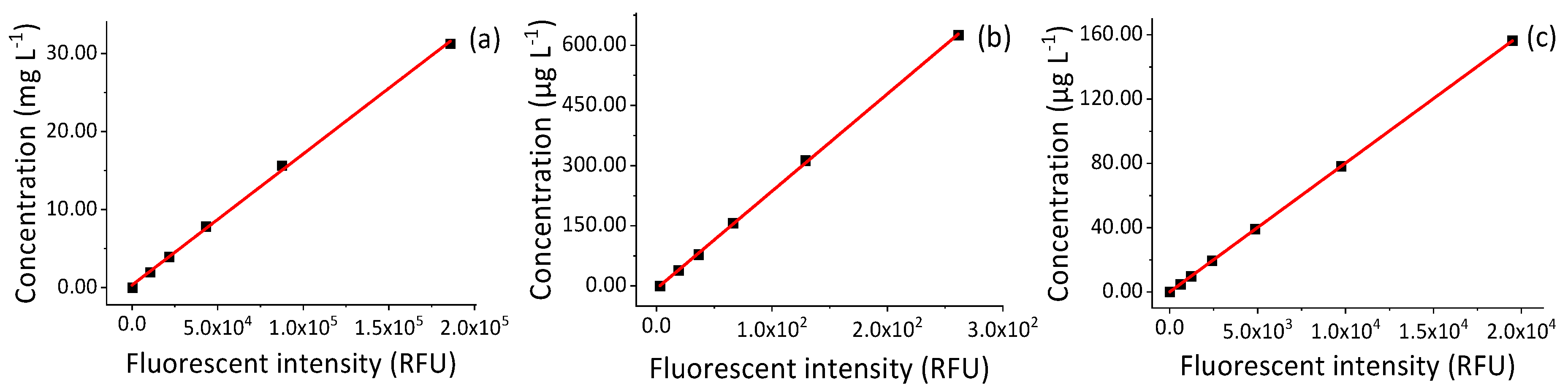
Figure 3.
The effect of temperature on the measured concentration of BSF solutions at nominal concentrations of 5.00, 10.00, 15.00, 20.00, 25.00, and 30.00 mg L−1 (error bars represent the doubled standard deviation (±2σ)).
Figure 3.
The effect of temperature on the measured concentration of BSF solutions at nominal concentrations of 5.00, 10.00, 15.00, 20.00, 25.00, and 30.00 mg L−1 (error bars represent the doubled standard deviation (±2σ)).

Figure 4.
The effect of temperature on the measured concentration of Eosin solutions at nominal concentrations of 37.50, 75.00, 150.00, 300.00, and 600.00 μg L−1 (error bars represent the doubled standard deviation (±2σ)).
Figure 4.
The effect of temperature on the measured concentration of Eosin solutions at nominal concentrations of 37.50, 75.00, 150.00, 300.00, and 600.00 μg L−1 (error bars represent the doubled standard deviation (±2σ)).

Figure 5.
The effect of temperature on the measured concentration of Fluorescein sodium salt solutions at nominal concentrations of 4.88, 9.77, 19.53, 39.06, 78.12, and 156.25 μg L−1 (error bars represent the doubled standard deviation (±2σ)).
Figure 5.
The effect of temperature on the measured concentration of Fluorescein sodium salt solutions at nominal concentrations of 4.88, 9.77, 19.53, 39.06, 78.12, and 156.25 μg L−1 (error bars represent the doubled standard deviation (±2σ)).
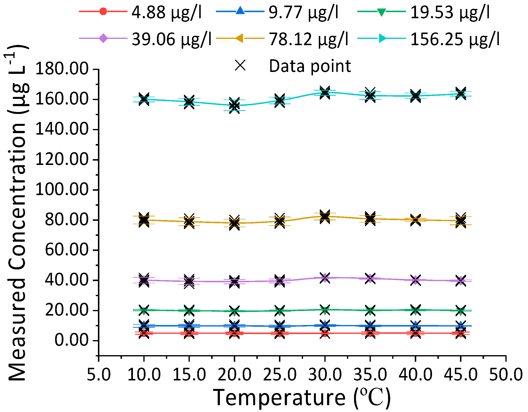
Figure 6.
Response surface graph for BSF, Eosin and Fluorescein sodium salt: (a) BSF; (b) Eosin; (c) Fluorescein sodium salt.
Figure 6.
Response surface graph for BSF, Eosin and Fluorescein sodium salt: (a) BSF; (b) Eosin; (c) Fluorescein sodium salt.

Figure 7.
Residual plots of the response surface graph: (a) BSF; (b) Eosin; (c) Fluorescein sodium salt.
Figure 7.
Residual plots of the response surface graph: (a) BSF; (b) Eosin; (c) Fluorescein sodium salt.

Figure 8.
Corrected concentrations: (a) BSF tracer; (b) Eosin; (c) Fluorescein sodium salt.


Table 1.
Fluorescent tracers used in the tests.
| Fluorescence Tracers | Excitation (nm) | Emission (nm) | CAS Number | Molecular Weight | Formula | Fluorescence Quantum Yield |
|---|---|---|---|---|---|---|
| BSF | 460 | 500 | 2391-30-2 | 404.4 | C19H13N2NaO5S | 0.27 |
| Eosin | 525 | 545 | 15086-94-9 | 647.9 | C20H8Br4O5 | 0.63 |
| Fluorescein sodium salt | 460 | 515 | 518-47-8 | 376.27 | C20H10Na2O5 | 0.97 |
Table 2.
Mean measured concentrations for BSF, Eosin and Fluorescein sodium salt solutions at different nominal concentrations across eight solution temperatures (10.0, 15.0, 20.0, 25.0, 30.0, 35.0, 40.0, and 45.0 °C).
Table 2.
Mean measured concentrations for BSF, Eosin and Fluorescein sodium salt solutions at different nominal concentrations across eight solution temperatures (10.0, 15.0, 20.0, 25.0, 30.0, 35.0, 40.0, and 45.0 °C).
| Fluorescent Tracer | BSF | ||||||
| Nominal concentration (mg L−1) | 5.00 | 10.00 | 15.00 | 20.00 | 25.00 | 30.00 | |
| Measured concentration (mg L−1) (CV (%)) | 4.3 (42.44) | 8.52 (47.58) | 12.83 (52.97) | 17.44 (56.90) | 22.74 (68.87) | 28.19 (78.18) | |
| Fluorescent tracer | Eosin | ||||||
| Nominal concentration (μg L−1) | 37.50 | 75.00 | 150.00 | 300.00 | 600.00 | ||
| Measured concentration (μg L−1) (CV (%)) | 42.64 (10.62) | 84.09 (10.32) | 164.37 (9.90) | 331.64 (10.68) | 655.93 (11.41) | ||
| Fluorescent tracer | Fluorescein sodium salt | ||||||
| Nominal concentration (μg L−1) | 4.88 | 9.77 | 19.53 | 39.06 | 78.12 | 156.25 | |
| Measured concentration (μg L−1) (CV (%)) | 4.90 (1.10) | 9.82 (1.37) | 20.04 (1.54) | 40.16 (2.26) | 79.91 (1.64) | 160.95 (1.79) | |
Table 3.
Mean corrected concentrations for BSF, Eosin and Fluorescein sodium salt solutions at different nominal concentrations across eight solution temperatures (10.0, 15.0, 20.0, 25.0, 30.0, 35.0, 40.0, and 45.0 °C).
Table 3.
Mean corrected concentrations for BSF, Eosin and Fluorescein sodium salt solutions at different nominal concentrations across eight solution temperatures (10.0, 15.0, 20.0, 25.0, 30.0, 35.0, 40.0, and 45.0 °C).
| Fluorescent Tracer | BSF | |||||
| Nominal concentration (mg L−1) | 5.00 | 10.00 | 15.00 | 20.00 | 25.00 | 30.00 |
| Corrected concentration (mg L−1) (CV (%)) | 4.68 (10.21) | 10.09 (1.76) | 15.22 (2.38) | 20.39 (2.94) | 25.04 (1.62) | 29.52 (2.62) |
| Fluorescent tracer | Eosin | |||||
| Nominal concentration (μg L−1) | 37.50 | 75.00 | 150.00 | 300.00 | 600.00 | |
| Measured concentration (μg L−1) (CV (%)) | 37.53 (3.51) | 75.59 (2.87) | 148.96 (1.19) | 300.74 (0.94) | 599.89 (0.88) | |
| Fluorescent tracer | Fluorescein sodium salt | |||||
| Nominal concentration (μg L−1) | 4.88 | 9.77 | 19.53 | 39.06 | 78.12 | 156.25 |
| Measured concentration (μg L−1) (CV (%)) | 4.90 (1.10) | 9.82 (1.39) | 20.04 (1.53) | 40.16 (2.26) | 79.91 (1.64) | 160.95 (1.79) |
© 2020 by the authors. Licensee MDPI, Basel, Switzerland. This article is an open access article distributed under the terms and conditions of the Creative Commons Attribution (CC BY) license (http://creativecommons.org/licenses/by/4.0/).
Share and Cite
MDPI and ACS Style
Zhang, Z.; Zhu, H.; Guler, H. Quantitative Analysis and Correction of Temperature Effects on Fluorescent Tracer Concentration Measurement. Sustainability 2020, 12, 4501. https://doi.org/10.3390/su12114501
AMA Style
Zhang Z, Zhu H, Guler H. Quantitative Analysis and Correction of Temperature Effects on Fluorescent Tracer Concentration Measurement. Sustainability. 2020; 12(11):4501. https://doi.org/10.3390/su12114501
Chicago/Turabian StyleZhang, Zhihong, Heping Zhu, and Huseyin Guler. 2020. "Quantitative Analysis and Correction of Temperature Effects on Fluorescent Tracer Concentration Measurement" Sustainability 12, no. 11: 4501. https://doi.org/10.3390/su12114501
Note that from the first issue of 2016, this journal uses article numbers instead of page numbers. See further details here.