Resource Use in Mariculture: A Case Study in Southeastern China
by

Tomás Marín
1, 
Jing Wu
1,
Xu Wu
2,3,
Zimin Ying
1,
Qiaoling Lu
1,
Yiyuan Hong
1,
Xiaoyan Wang
1 and
Wu Yang
1,* 1
College of Environmental and Resource Sciences, Zhejiang University, Hangzhou 310058, China
2
Zhejiang Economic Information Center, Hangzhou 310006, China
3
College of Economics, Zhejiang University, Hangzhou 310058, China
*
Author to whom correspondence should be addressed.
Sustainability 2019, 11(5), 1396; https://doi.org/10.3390/su11051396
Submission received: 26 January 2019
/
Revised: 16 February 2019
/
Accepted: 26 February 2019
/
Published: 6 March 2019
(This article belongs to the Section Sustainable Agriculture)
Abstract
:China is the biggest provider of aquaculture products, and the industry is still growing rapidly. Further development of the sector will affect the provision of ecosystem services that maintain the livelihood of local populations. In particular, the current size and growth rate of China’s mariculture has raised many environmental concerns, but very few studies of this sector have been conducted to date. Here, we report the resource use in the production of six main Chinese mariculture products (Larimichthys crocea, Apostichopus japonicus, Haliotis spp., Laminaria japonica, Gracilaria spp., Porphyra spp.), taking the city of Ningde as a case study. We used the life cycle assessment framework and the Cumulated Exergy Demand indicator to quantify resource use, and implemented a Monte Carlo simulation where model uncertainty was included using various methods. The mean exergy demand values of the production of one live-weight ton of large yellow croaker, sea cucumber, abalone, laminaria, gracilaria, and porphyra are 106 GJ eq., 65 GJ eq., 126 GJ eq., 0.25 GJ eq., 1.55 GJ eq., and 0.98 GJ eq., respectively. For animal products, 45–90% of the impacts come from the feed requirements, while in seaweed production, 83–99% of the impacts are linked to the fuel used in operation and maintenance activities. Policies oriented toward efficient resource management in the mariculture sector thus should take the farm design, input management, and spatial planning of marine areas as the main targets to guide current practices into more sustainable ones in the future. Improvements in all those aspects can effectively increase resource efficiency in local mariculture production and additionally reduce other environmental impacts both locally and globally.
1. Introduction
Aquaculture is an important sector in the food industry. It constitutes a source of both income and livelihood to 19.4 million people and it is currently among one of the main sources of growth in the food industry worldwide [1]. This is the result of the increase in the demand for aquatic products, the improvement of distribution channels, and the limited capacity of wild fisheries to meet the rising demand. This rapid growth has generated numerous concerns about the environmental impacts caused by this industry.
The development of aquaculture in coastal and marine locations has become a big issue in sustainable development. These areas have important ecological functions, including the support of fisheries and nursery habitats, the development of coastal land, the support of recreation, tourism, and retirement industries, the recycling of global materials, the transformation, detoxification, and sequestration of pollutants and societal wastes, the provision of cultural and future scientific values, and the provision of raw materials [2,3,4]. The expansion of aquaculture into these areas affects the local environment in several ways. First, it changes the land use and land cover both in the land and the sea [5]. Second, it increases the release of organic and chemical waste effluents as well as the risk of escaped species and diseases into the local environment [5]. Third, it aggravates the pressure on natural resources, such as water, energy, and land, both locally and globally [6,7]. Resource overexploitation and environmental pollution by the development of the aquaculture industry thus will impair the function of all those ecosystems linked to the supply chain of aquaculture production. These negative consequences will also have socioeconomic impacts, because the welfare of the people involved in aquaculture activities depends on the productive capacity of these ecosystems to supply aquatic products in adequate quantities and with satisfactory quality. This supply constitutes both a direct subsistence resource and the source of income for many communities, particularly in underdeveloped areas [5,8]. All these environmental impacts thus may harm these stocks of natural resources and aggravate poverty issues in the long term.
As the biggest provider of aquaculture products in the world, China is particularly vulnerable to these impacts [9]. As a result, some case studies of inland and coastal aquaculture have been conducted in this country from a systems perspective. Most of these publications have assessed the environmental burden of inland aquaculture systems [10,11,12,13,14], which play a central role in the Chinese aquaculture and include important products, such as shrimp and tilapia [15,16]. However, these studies have considered products farmed in fresh and brackish water systems, and very few have focused on the environmental impacts of Chinese mariculture. The impacts of these systems can be disproportionately large in relation to its production volume as a result of the dependence on wild fish for feed, the introduction and spread of invasive species, and the generation of marine pollution [17,18]. The magnitude of the environmental impacts due to mariculture production is likely to increase in the next years due to the rapid expansion of the sector, with an average growth rate of 6% in the annual production between 2011 and 2016 [19]. This industry is expected to supply the majority of the total marine production in China in the future [20], as the productivity of wild fisheries is not expected to increase [1]. Moreover, previous studies have already highlighted the impact of anthropogenic activities in the marine areas of China as being among the highest in the world [21], and the Chinese Government is currently promoting policies to make this sector, and aquaculture production in general, a more sustainable industry [1]. More studies on the environmental burden caused by this growing industry and its effects on sustainable development are thus necessary.
The main objective of this study is to quantify the resource use due to mariculture production in the city of Ningde, one of the main centers of mariculture production in China. For this purpose, we conducted a life cycle assessment (LCA) of the main mariculture products farmed in the area and calculated the amount of resources required in their production. The analysis of these results will raise the current challenges and opportunities in resource use and management in the systems under study. The findings of this case study also aim to serve as a reference of the current trends of the environmental impacts of mariculture in China.
2. Materials and Methods
2.1. Study Area
Ningde city (N 26°39′42″ E 119°31′23″) is a coastal prefecture-level city located in Fujian province (Figure 1). The total aquaculture production in its coastal and marine areas accounts for 20% and 4.5% of the total coastal and marine aquaculture production in Fujian and China, respectively [22]. A wide complex of farms is currently installed in the sea and its surrounding areas, and approximately 475 km2 of the sea surface is occupied by mariculture systems [22]. Although there are a few commercial farms, most farms are managed by individual households who sell their products to the local markets and intermediary traders. A wide variety of animal and seaweed species are farmed in the sea, including many characteristic products of the area. Many of these products have high socioeconomic importance among the local agricultural products as they constitute one of the main sources of income of a big proportion of the local population. However, to the best of our knowledge, very few environmental assessments of this rapidly growing industry have been conducted.
2.2. Survey Data
We conducted a survey in August 2017 and January 2018 in which we interviewed a total of 321 households in the four coastal administrative districts of Ningde (Figure 1). During the survey, we selected the household heads or their spouses as interviewees because they are most familiar with the farming practices. We surveyed household demographic information (e.g., household size, educational level, gender, education) and aquaculture production data (e.g., products, farmed area, production volume, unit price, gross income, and material and labor expenditures). In this study, we focused on the main mariculture products farmed in the area during 2016. From these households, we chose those products that account for more than 2% of the total number of records (mixed finfish was excluded because it includes many species). A total of six products were thus included in our assessment: Large yellow croaker (Larimichthys crocea), sea cucumber (Apostichopus japonicus), abalone (Haliotis spp.), laminaria (Laminaria japonica, commonly referred to as kelp), gracilaria (Gracilaria spp.), and porphyra (Porphyra spp., commonly referred to as nori) (Table 1). For large yellow croaker and sea cucumber, products were further classified into categories according to the type of feeds reported in the survey.
2.3. Description of the Aquaculture Production Process
The main aquaculture production chain has four stages: Broodstock collection, seed production, seed nursery, and juvenile grow-out. Broodstock is first collected from natural or aquaculture stocks and transported to a hatchery, where fry, spats, and sporelings are produced in controlled conditions. The seeds are either kept in the hatchery for nursery before being transported to farms for grow-out or sold directly to nursing farms outside the hatchery. Transport is done via small lorries and boats, which carry the seeds in plastic bags or water tanks to the farms for nursery or grow-out.
In Ningde, grow-out stages are completed on marine farms (for sea cucumber and abalone, other systems are also commonly used in other provinces of China, see [23] and [24]). Cage farms are used for animal species while raft farms are used for seaweed. The cage system for finfish consists of a wooden grid where fish is farmed inside a net layer which hangs into the water between the frames. For non-finfish animals, the cage system consists of a plastic cage, which holds a number of individuals inside. Besides the frames, cage farms usually include areas where auxiliary tools and machinery are kept. The raft system consists of a group of ropes with attached seaweed seeds deployed in the sea surface. This system usually uses plastic bottles to float and a mooring system keeps the farms in a fixed location. In Ningde, most products are farmed in monoculture systems. However, some farms have polyculture systems where many species are produced together, particularly finfish farms. For instance, in some farms, the large yellow croaker is produced together with black porgy (Sparus macrocephlus) and rainbow trout (Oncorphynchus mykiss) in multi-layer nets.
In the production of animal products, an active trade of intermediate products (juveniles of various sizes) exists. Some farmers often buy seeds and small juveniles to farm them for a period of time, and then sell them as a larger juvenile, depending on the season and the species. In particular, the juveniles of sea cucumber and abalone are commonly traded and transported to areas where the seawater temperature is more adequate for further growth. They are usually transported to northern provinces during summer and to southern provinces during winter [24,25].
One of the main inputs required for animal species is the feedstuff and it can be classified into two types: Formulated feed and artisanal feed. The formulated feed is manufactured by an external company from processed ingredients based on a specific formula. There is a wide variety of feeds available in the market, ranging from generic feeds to highly specific feeds. All these can differ in price, quality, and composition. The artisanal feed is produced on-site by the farmers themselves based on ingredients with minimal processing. Differences in the composition of artisanal feed can also vary widely due to the availability and quality of ingredients in each case.
As a process that is highly dependent on the ecosystem, local mariculture production can be highly heterogeneous. Natural factors, such as weather, season, and geographical location, all have a significant influence on the process. Other factors, such as the availability of inputs, equipment, infrastructure, and personal practices, in each stage of the production chain also have effects on the production process.
2.4. Life Cycle Assessment Model
Our model was based on the LCA framework, defined by the International Organization for Standardization (ISO14044) standard as the compilation and evaluation of the inputs, outputs, and potential environmental impacts of a product throughout its life cycle [26,27]. This method has already been successfully applied to a number of aquaculture systems to measure the environmental impacts of different products through a number of indicators [28,29]. We conducted our assessment on each of the products selected from cradle-to-farm-gate and took one live-weight ton of product as the functional unit. The main objective of our analysis was to estimate the average resource consumption of the species farmed in Ningde. Therefore, the analysis took an attributional approach and included the production of fry, spat, and sporelings in the hatchery, the nursery of seeds, the grow-out of juveniles, and the feed production (Figure 2). We also included the production and supply of energy inputs, feed ingredients, transport services, and other minor inputs required in the process. Infrastructure and equipment were not included because of the high efforts needed for data collection in relation to their impact on the final values [30]. Broodstock collection was also not included due to the lack of reliable data and to the small contribution it may have on the final results.
We constructed a life cycle inventory of mariculture production both from survey data and scientific references. We collected primary data for the grow-out stages and secondary data to model other processes, such as seed and juvenile production, feed production, and transport requirements. We used allocation by mass throughout our analysis, following recommended guidelines [31]. More details about primary data analysis, secondary data sources, and input allocation can be found in the Supplementary Materials.
The life cycle impact assessment took the Cumulated Exergy Demand (CExD) as the indicator for our analysis [32]. The CExD indicator represents the exergy of natural resources required throughout the life cycle of a product. It accounts for energy inputs and non-energy inputs, such as metal ores, minerals, and water [32]. Exergy-based approaches in the LCA of aquaculture systems are relatively recent, and only a few related studies have been published to date [33,34,35,36,37]. We obtained the impacts’ factors of the background processes from the Ecoinvent database (v.3.5) [38]. Although there are more comprehensive indicators, such as the Cumulative Exergy Extraction from the Natural Enviroment [39], in this work, we did not consider them for practical reasons because no models for these indicators were available within the newest versions of the Ecoinvent database. The specific datasets and estimated values used as impact factors can be found in the Supplementary Materials.
To account for the variability of the system under study, we implemented a Monte Carlo simulation [40] in the R software (v.3.3.2) [41]. Each unit process was characterized by a set of input parameters, a geographical location, and, for the grow-out stages, a correlation matrix. We used 2000 iterations in the simulation, and included the variability of the unit processes due to inherent uncertainty, spread, and unrepresentativeness [42]. Inherent uncertainty was included by assuming a coefficient of variation of 5% [36], spread was calculated from primary and secondary data, and unrepresentativeness was addressed by using the Pedigree approach [43,44]. The correlation between process chains was included by using dependent sampling in each iteration [45], and the correlation between process variables was addressed by using copula functions (package “copula” [46]) to model the relationship between the variables of a unit process.
To model the correlation among variables of a unit process in the LCA, we used copula functions to obtain the correlated instances in each Monte Carlo iteration. A copula is a multivariate probability distribution function represented by two or more uniform marginal probability distributions [47]. A process unit can thus be modeled in terms of the univariate marginal distributions of each parameter and a copula function, where the former describes the distribution of the individual random variables and the latter describes the relationship between these variables. To describe the correlations between the unit process variables in the simulation, we employed the Spearman’s rank correlation coefficient. We included correlations among the variables in the grow-out stages by using the correlation matrix from our primary data, and assumed the correlations among the variables for the other processes to be zero. Because our data were not sufficient to fit an optimal copula among the existing functions, we obtained correlated instances using a t-copula.
Although some previous studies [48,49] have included correlations among process variables in the LCA, it is not a standard practice. Consequently, we constructed two versions of the LCA model, where correlations among variables were ignored in one (uncorrelated model) and included in the other (correlated model). We ran each version 100 times to estimate the variability of the median and the standard error of the total exergy demand for each product. We used identical random sampling in both models. We considered that the correlated model should give more accurate estimates, and we thus showed and analyzed the inventory and impact assessment calculated from the correlated model. These final results correspond to the mean of the 100 values calculated for each parameter.
Due to the complexity of the local mariculture industry, we had to use a number of assumptions to construct our simulation. In the model, we assumed that all the biomass increase is sold as a finished product, but in animal farming (grow-out stages), a part of the production is composed by juveniles, which do not enter the market as a fully-grown product, but are either sold to other farms or kept at the same farm for further growth. Moreover, we considered that the environmental burden of production losses (e.g., fallen stock, fish escape, etc.) are attributed to the production output. This way, the assessment reflects the performance of the farms in terms of the inputs required to obtain a given output, including losses. Furthermore, we assumed an average process for the production of seeds and juveniles with well-defined stages of growth (Table 2). Finally, we used a sampling procedure in each iteration to specify the source of a specific input, where the probability for an input to come from a particular location was equal to the proportion of the total production volume of that location. This accounts for differences in the distances traveled by inputs between stages and in the impact factors of equivalent inputs in different areas (e.g., electricity). We considered this procedure only for calculation purposes and the final results (inventories and impact assessment) are shown as aggregated values.
2.5. Statistical Analysis
Dependent sampling allows for paired statistical tests, which gives more statistical power compared with independent sampling in the analysis of the results of Monte Carlo simulations [45]. Due to the non-normality of most of the data, we used the Wilcoxon signed-rank test to explore differences between samples. This test allows an estimate for the pseudomedian (i.e., the difference in the location parameters between two samples) to be obtained, and also establishes whether differences between samples are statistically significant.
3. Results
3.1. Comparison between Correlated and Uncorrelated Model Versions
The parameter estimates obtained from the correlated and uncorrelated models are different from each other for most products (see Supplementary Materials Table S21 for details). Moreover, a comparison between the models using the Wilcoxon signed-rank test shows that these differences are statistically significant in some cases. By including correlations among variables, the statistically significant median values and standard errors decreased by 1.0–6.5% (Figure 3) and 2.6–18.4% (Figure 4), respectively. The product with the biggest difference between the median values is gracilaria, followed by abalone and sea cucumber (Figure 3). For standard error values, considerable differences occur in sea cucumber, abalone, and gracilaria production, with a relatively small difference for large yellow croaker (Figure 4).
3.2. Life Cycle Inventory
The life cycle inventory reflects the different input requirements and the economic feed conversion ratio (FCR, the ratio between the total amount of feed used and the total biomass obtained) for each product (Table 3 and Table 4). For animal products, most of the material requirements are due to the feed, whereas in seaweed production, the fuel used in operation and maintenance activities constitutes the bulk of the material requirements. The inventory also shows that most farmers in Ningde have a preference towards the artisanal feed, and formulated feed is used in comparatively small quantities. Moreover, the estimates for the FCR values are high and show that the amounts of feed used are considerably bigger than the amount of biomass obtained from the process. The survey also showed that a number of chemical products are used in the area, including antimicrobials (e.g., oxytetracycline dehydrate) and probiotics (e.g., bacteria powder). However, the data available do not specify the type of chemicals used and were thus considered together as one type of input.
3.3. Life Cycle Impact Assessment
The total exergy demand disaggregated by the inputs required along the process show distinct patterns for each product (Figure 5). On average, feed inputs account for 45–90% of the total exergy demand in animal production, the proportion being the lowest for abalone (46%), intermediate for sea cucumber (58–71%), and the highest for large yellow croaker (87–89%). Most of this exergy demand comes from the fuel required in the production of trash fish and raw seaweed used as feed. The production of small juveniles of yellow croaker, sea cucumber, and abalone contributes 6–9%, 11–16%, and 26% of the total exergy demand value, respectively. For seaweed products, the main source of impacts comes from the use of fuel in the farming stage, accounting for 83–99% of the total exergy demand, and impacts from other inputs are comparatively small. The figure also indicates that seeds and juveniles are often produced in other areas, and that impacts due to production are thus distributed between different geographical regions. This is particularly the case for sea cucumber and abalone, whose impacts due to seed and small juvenile production are considerable when compared to their total exergy demand.
The total exergy demand for each product also shows distinctive trends in terms of the central tendency and variability (Figure 6). The mean and standard error values for the total exergy demand of animal production are 115 ± 86 GJ eq. and 97 ± 68 GJ eq. for yellow croaker (categories A1 and A2, respectively), 84 ± 44 GJ eq., 65 ± 46 GJ eq., and 45 ± 30 GJ eq. for sea cucumber (categories B1, B2, and B3, respectively), and 126 ± 158 GJ eq. for abalone, respectively. The corresponding mean and standard error values for seaweed production are 0.25 ± 0.32 GJ eq. for laminaria, 1.55 ± 2.83 GJ eq. for gracilaria, and 0.98 ± 1.04 GJ eq. for porphyra, respectively (Figure 6). For all products, the primary resources required in the productive process come mostly from the fossil energy category (Figure 7). Biomass and water resources have a fair contribution for animal products, and the share of the other impact categories is comparatively low for all products.
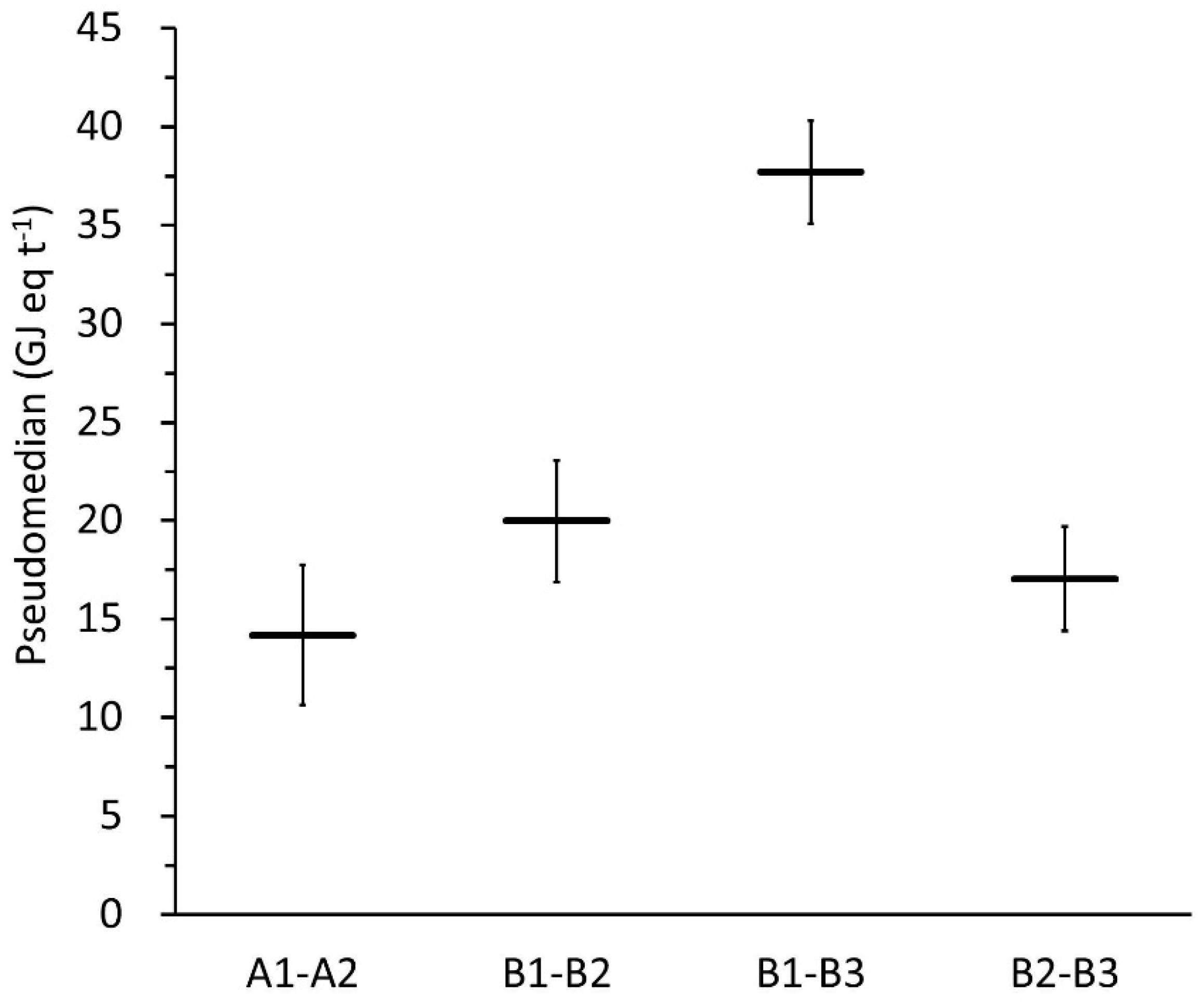
The comparison between categories shows that the environmental impacts in the farms that use artisanal feeds are lower in magnitude to those farms that use formulated feeds (Figure 8). For both large yellow croaker and sea cucumber, the results of the paired tests show a significant difference between the categories in terms of their resource consumption.
4. Discussion
We assessed the resource use in the production of the six most important mariculture products in Ningde by calculating the total exergy demand of the production process in each case. Our findings show that each product has distinctive patterns of resource use. Below we discuss these results and their main implications on resource management and environmental protection.
4.1. Local and Global Impacts of Resource Use
The source of inputs required for aquaculture production commonly include both local and remote locations, particularly when feed is required. In our analysis, remote impacts from the local mariculture industry are mainly due to the production of seeds and juveniles and of formulated feed. Remote impacts due to feed production have already been identified in many reports [58,59,60], and the results of our assessment indicate that seed and juvenile production may also have impacts on remote locations.
The feed type used in mariculture production (formulated or artisanal feed) is closely related to both the magnitude and location of the corresponding environmental impacts. For artisanal feeds, most of its environmental impacts occur at a local level, because it is both produced and utilized by the local industry. Its use pollutes the water, makes farmed individuals more susceptible to diseases, reduces the quality and quantity of the harvested products, and increases the pressure on wild fish resources [20,61,62]. On the other hand, the impacts due to the use of formulated feeds occur in remote locations, particularly in the areas where the production of its ingredients takes place. For example, the formulated feed of yellow croaker and sea cucumber have fish-derived and soybean sub-products among their ingredients. Most of the production of these ingredients occurs in North and South America and they are imported to China [63]. Therefore, there is a tradeoff between the impacts of formulated feed and artisanal feed. Artisanal feeds have comparatively higher impacts (e.g., water pollution) on the local environment. Formulated feeds, although having lower environmental impacts at the local level, generate impacts in those areas where the feed ingredients are extracted, processed, and imported to China [64].
Seed and juvenile production also have spillover effects on remote places. For some species, many of the seeds and juveniles are produced outside the area of study [19]. This is particularly the case for sea cucumber and abalone production, both being species traditionally farmed in Northeastern China. The farmers of these products have adopted the practice of carrying out part of the grow-out stages in Southeastern China (including Ningde) during winter months, when the water temperature is more favorable for the growth of juveniles [24,25].
4.2. Input Management
The life cycle assessment results reflect the different trends among households in the amount and type of inputs used and their environmental impacts. In general, the variability in the amount of inputs used points to the lack of standard practices, the low degree of formal input management, and the natural variability of the process (species requirements, environmental factors, etc.). In animal farming, the use of artisanal feeds is a widespread practice in the surveyed area due to its cost, its availability, and to personal preferences. The FCR values of feed categories and the proportion between feed types suggests that formulated feed is mostly used in the production of small juveniles and that the bulk of feed requirements is thus satisfied by using artisanal feeds. Additionally, the comparison between feed categories suggests that the use of different feed types is related to different magnitudes of environmental impacts. In seaweed farming, most of the resource use and associated impacts are due to fuel usage. All these findings highlight the need to improve the management of these inputs in the local mariculture industry.
For animal products, feed constitutes the main source of resource consumption. This is consistent with previous studies, where the feed is highlighted as the main source of environmental impacts in open water systems [29]. The need to optimize the production and management of feedstuff has already been highlighted in several studies [16,60,65,66], and the high values of the estimated FCR values also point to the need to improve the efficiency of feed usage. Feed management is thus one of the key factors to enhance the performance of local cage mariculture, and not only contributes to the reduction of resource use, but also helps to attenuate other environmental impacts. Improvements in efficiency may be achieved by using polyculture systems, where the outputs and excess feed of one species can be consumed by another species. Polyculture farm designs have already been implemented in some farms of Ningde, where finfish is farmed in multilayer nets and different species are farmed in different water levels. Moreover, this design can be complemented with other measures to reduce the impacts of the farming effluents, such as the use of detritivorous fish and invertebrates to harvest organic matter from the enriched seabed, or the use of pelagic biofilters around aquaculture cages to reduce the local environmental load and obtain a valuable sub-product [9,67].
In the case of seaweed species, the main source of impact is the fuel required in operation activities. Fuel consumption is mainly determined by the frequency of operation activities and on the distances covered by each farmer. For some households, it also depends on the number of products a household is producing, because many households farm more than one product and different products are often not farmed in the same location. Hence, both the standardization of operations and improvements in local spatial planning can help to reduce the distances covered in the trips. To the best of our knowledge, no centralized efforts have been done to optimize local mariculture production, and spatial planning and management of the marine areas plays a key role in sustainable practices [68]. As laminaria and porphyra both constitute ingredients for feed, an efficient use of fuel in daily operations will also reduce the resource requirements for the production of other species.
Overall, individual practices and system design all play a role in the efficient management of resource use, and the results of this study point to the need to implement formal training programs and to establish and improve standard practices in farming operations. Further increases in production will make it necessary to regulate the use of feed and chemicals to preserve the integrity of the local ecosystem.
4.3. Correlation among Unit Process Variables
In our study, the model results only included the correlation among process variables in the grow-out stages, and the correlations in other processes were not considered. Nevertheless, our results show that this type of correlation may affect the estimated results, particularly in the parameters describing the variability of the system. When the variables describing the inputs and outputs of a process are correlated to each other to some extent, both the sampling space and simulation results change accordingly when LCA models account for this effect [48]. The approach we took in this study allows the integration of this correlation within the standard framework of LCA studies, where Monte Carlo simulations are often based on marginal distribution data for each variable. However, the decision of whether to include correlations among process variables in other studies should mainly depend on two factors. First, the characteristics of the specific system under study and the importance of the correlation among its variables should be considered. Previous knowledge and preliminary analyses can help to establish whether it is worthwhile to include this effect in the model. As shown in our work, the change in the results can be comparatively small in some cases, and other methodological choices may be of more relevance (e.g., allocation criteria). Second, the amount of data required should also be considered. The data required to obtain reliable estimates of the correlation coefficients is considerable, and may render this method as unfeasible in those cases where data availability is limited.
4.4. Limitations
We identified two main limitations of our results. First, we did not include human labor nor land use in the analysis. Human labor usually is not considered in the analysis of aquaculture production systems, but it is a relevant factor in the local industry because it is one of the key requirements of the production process. With respect to land and marine occupation, its importance in agriculture and aquaculture production suggests that the impacts of the local aquaculture industry are higher than our estimations, as suggested by previous studies [34,69]. Although some indicators have been created to account for these factors [39,70,71], none have been formally integrated in the most recent Ecoinvent databases and they were not considered in our analysis for practical reasons.
Second, we also acknowledge limitations in our model due to the available data and to the simplifications and methodological choices made to address time horizons, spatial variation, and system dynamics in the model. For instance, the modeling of some processes, particularly in the production of sea cucumber and abalone juveniles, is partly based on experimental data and discrepancies between our estimates and real data may exist. Likewise, unit process locations were obtained from available publications and they only constitute an estimate. Much more detailed data would be necessary to perform a more complete analysis and overcome some of these limitations, many of which arise from the inherent problems of the LCA framework [27]. Despite these shortcomings, we consider that our results constitute a representative estimate of the environmental impacts of the local mariculture due to resource use.
4.5. Future Research
We identified several issues for further investigation. First, future research should conduct a more comprehensive assessment by including other indicators (e.g., eutrophication, seafloor damage, biodiversity loss, and microplastic pollution) that may be relevant in our area of study. Such an analysis could give additional insights about the environmental impacts of the local mariculture industry. Second, we identify the need for a systematic study about polyculture systems in the area under study. Polyculture systems are not commonly employed and an analysis of the feasibility and benefits of these systems in the local context could provide valuable input to local policy. Thirdly, future work should also explore alternative feed formulations for animal products and their environmental impacts, similar to what has already been done for salmonids [60,69,72,73]. A more detailed assessment is necessary to provide concrete guidelines to produce more sustainable feeds. Such a study could also quantify the impacts of each ingredient in different locations and account for the tradeoff between local and remote impacts due to feed use. Finally, further research can also take a coupled human and natural systems approach [74,75] to identify the causal mechanisms of the rapid expansion of Chinese aquaculture in coastal areas, and its associated environmental and socioeconomic impacts in other places around the world. This is critical to the long-term management of the local aquaculture industry as well as global sustainability.
5. Conclusions
The rapid growth of mariculture production in China places an increasing pressure on natural resources and is also increasing environmental damage, generating significant impacts across local, national, and global scales. Our study assessed the exergy demand of some of the main local species from a life cycle perspective to find the main environmental hotspots of the process. Our results show that the main contributors to resource use in animal and seaweed production are feed and fuel, respectively. Feed represents 45–90% of the environmental impacts of animal mariculture, and fuel accounts for 83–99% of the environmental impacts due to seaweed production. Policies oriented to improve resource management should thus take feed and fuel consumption as the main targets to guide current practices into more sustainable ones. Improvements in farm design and management can effectively reduce the resource consumption of the production process. Likewise, improvements in training programs, production standards, and spatial planning are also necessary to improve the efficiency of local mariculture production. These measures may additionally reduce other environmental and socioeconomic impacts, both at the local and global scales.
Supplementary Materials
The following are available online at https://www.mdpi.com/2071-1050/11/5/1396/s1, Table S1: Summary of the data used to calculate allocation parameters, Table S2: Distributions and parameters used to fit the primary data of the case study, Tables S3–S18: Distribution parameters and correlation matrices of each farming process, Table S19: Data sources for the life cycle inventory of feed production, Table S20: Data sources for the life cycle inventory of the main chain of mariculture production, Table S21: Parameters of the total exergy demand calculated from the uncorrelated and the correlated model, Table S22: Ecoinvent models used in the life cycle impact assessment of the case study. R scripts are available under request.
Author Contributions
Funding acquisition, W.Y. and X.W. (Xu Wu); investigation, J.W., Z.Y., Q.L., Y.H., X.W. (Xiaoyan Wang), and W.Y.; methodology: T.M. and W.Y.; formal analysis, T.M.; writing—original draft preparation, T.M.; writing—review & editing, T.M., X.W. (Xu Wu), and W.Y.; supervision, W.Y.
Funding
This research was funded by the National Natural Science Foundation of China (71673247), Ministry of Science and Technology of China (2016YFC0503404), Outstanding Youth Fund of Zhejiang Province (LR18D010001), and Zhejiang Provincial Natural Science Foundation (LQ18G030002).
Acknowledgments
We thank Thomas Schaubroeck for his helpful comments on an earlier draft.
Conflicts of Interest
The authors declare no conflict of interest.
References
- FAO. The State of World Fisheries and Aquaculture 2018—Meeting the Sustainable Development Goals; FAO: Roma, Italy, 2018. [Google Scholar]
- Barbier, E.B.; Hacker, S.D.; Kennedy, C.; Koch, E.W.; Stier, A.C.; Silliman, B.R. The value of estuarine and coastal ecosystem services. Ecol. Monogr. 2011, 81, 169–193. [Google Scholar] [CrossRef] [Green Version]
- Kaufman, L.; Dayton, P. Impacts of marine resource extraction on ecosystem services and sustainability. In Nature’s Services: Societal Dependence on Natural Ecosystems; Daily, G.C., Ed.; Island Press: Washington, DC, USA, 1997. [Google Scholar]
- Peterson, C.H.; Lubchenco, J. Marine Ecosystem Services. In Nature’s Services: Societal Dependence on Natural Ecosystems; Daily, G.C., Ed.; Island Press: Washington, DC, USA, 1997. [Google Scholar]
- Little, D.C.; Newton, R.W.; Beveridge, M.C.M. Aquaculture: A rapidly growing and significant source of sustainable food? Status, transitions and potential. Proc. Nutr. Soc. 2016, 75, 274–286. [Google Scholar] [CrossRef] [PubMed]
- Dasgupta, P.S.; Ehrlich, P.R. Pervasive Externalities at the Population, Consumption, and Environment Nexus. Science 2013, 340, 324–328. [Google Scholar] [CrossRef] [PubMed]
- Liu, J.; Yang, W.; Li, S. Framing ecosystem services in the telecoupled Anthropocene. Front. Ecol. Environ. 2016, 14, 27–36. [Google Scholar] [CrossRef]
- Sumaila, U.R.; Bellmann, C.; Tipping, A. Fishing for the future: An overview of challenges and opportunities. Mar. Policy 2016, 69, 173–180. [Google Scholar] [CrossRef]
- Liang, Y.X.; Cheng, X.W.; Zhu, H.; Shutes, B.; Yan, B.X.; Zhou, Q.W.; Yu, X.F. Historical Evolution of Mariculture in China During Past 40 Years and Its Impacts on Eco-environment. Chin. Geogr. Sci. 2018, 28, 363–373. [Google Scholar] [CrossRef]
- Garcia, F.; Kimpara, J.M.; Valenti, W.C.; Ambrosio, L.A. Emergy assessment of tilapia cage farming in a hydroelectric reservoir. Ecol. Eng. 2014, 68, 72–79. [Google Scholar] [CrossRef]
- Liu, J.; Zhou, H.P.; Qin, P.; Zhou, J.; Wang, G.X. Comparisons of ecosystem services among three conversion systems in Yancheng National Nature Reserve. Ecol. Eng. 2009, 35, 609–629. [Google Scholar] [CrossRef]
- Zhang, L.X.; Song, B.; Chen, B. Emergy-based analysis of four farming systems: Insight into agricultural diversification in rural China. J. Clean. Prod. 2012, 28, 33–44. [Google Scholar] [CrossRef]
- Lu, H.F.; Tan, Y.W.; Zhang, W.S.; Qiao, Y.C.; Campbell, D.E.; Zhou, L.; Ren, H. Integrated emergy and economic evaluation of lotus-root production systems on reclaimed wetlands surrounding the Pearl River Estuary, China. J. Clean. Prod. 2017, 158, 367–379. [Google Scholar] [CrossRef] [PubMed]
- Shi, H.H.; Zheng, W.; Zhang, X.L.; Zhu, M.Y.; Ding, D.W. Ecological-economic assessment of monoculture and integrated multi-trophic aquaculture in Sanggou Bay of China. Aquaculture 2013, 410, 172–178. [Google Scholar] [CrossRef]
- Cao, L.; Diana, J.S.; Keoleian, G.A.; Lai, Q. Life Cycle Assessment of Chinese Shrimp Farming Systems Targeted for Export and Domestic Sales. Environ. Sci. Technol. 2011, 45, 6531–6538. [Google Scholar] [CrossRef] [PubMed]
- Cao, L.; Naylor, R.; Henriksson, P.; Leadbitter, D.; Metian, M.; Troell, M.; Zhang, W. China’s aquaculture and the world’s wild fisheries. Science 2015, 347, 133–135. [Google Scholar] [CrossRef] [PubMed]
- Bostock, J.; McAndrew, B.; Richards, R.; Jauncey, K.; Telfer, T.; Lorenzen, K.; Little, D.; Ross, L.; Handisyde, N.; Gatward, I.; et al. Aquaculture: Global status and trends. Philos. Trans. R. Soc. B Biol. Sci. 2010, 365, 2897–2912. [Google Scholar] [CrossRef] [PubMed]
- Volpe, J.; Gee, J.; Ethier, V.; Beck, M.; Wilson, A. Global Aquaculture Performance Index (GAPI): The First Global Environmental Assessment of Marine Fish Farming; University of Victoria: Victoria, BC, Canada, 2010. [Google Scholar]
- Fishery Policy and Administration Bureau, Ministry of Agriculture of China. China Fisheries Yearbook; China Agriculture Press: Beijing, China, 2012–2017. (In Chinese)
- Chen, J.X.; Guang, C.T.; Xu, H.; Chen, Z.X.; Xu, P.; Yan, X.M.; Wang, Y.T.; Liu, J.F. A review of cage and pen aquaculture: China. In Cage Aquaculture—Regional Reviews and Global Overview; Halwart, M., Soto, D., Arthur, J.R., Eds.; FAO Fisheries Technical Paper No. 498; FAO: Rome, Italy, 2007; 241p. [Google Scholar]
- Halpern, B.S.; Walbridge, S.; Selkoe, K.A.; Kappel, C.V.; Micheli, F.; D’Agrosa, C.; Bruno, J.F.; Casey, K.S.; Ebert, C.; Fox, H.E.; et al. A global map of human impact on marine ecosystems. Science 2008, 319, 948–952. [Google Scholar] [CrossRef] [PubMed]
- Ningde Municipal Statistical Bureau. Ningde Statistical Yearbook; China Statistical Press: Beijing, China, 2017.
- Han, Q.; Keesing, J.K.; Liu, D. A Review of Sea Cucumber Aquaculture, Ranching, and Stock Enhancement in China. Rev. Fish. Sci. Aquac. 2016, 24, 326–341. [Google Scholar] [CrossRef] [Green Version]
- Wu, F.; Zhang, G. Pacific Abalone Farming in China: Recent Innovations and Challenges. J. Shellfish Res. 2007, 35, 703–710. [Google Scholar] [CrossRef]
- Jiang, S.; Ren, Y.; Tang, B.; Li, C.; Jiang, C. Development status and countermeasures of Apostichopus japonicus culture industry in China. J. Agric. Sci. Technol. 2017, 19, 15–23. [Google Scholar]
- International Organization for Standardization. ISO 14044:2006 Environmental Management—Life Cycle Assessment—Requirements and Guidelines; International Organization for Standardization: Geneva, Switzerland, 2006. [Google Scholar]
- International Organization for Standardization. ISO 14040:2006 Environmental Management—Life Cycle Assessment—Principles and Framework; International Organization for Standardization: Geneva, Switzerland, 2006. [Google Scholar]
- Cao, L.; Diana, J.S.; Keoleian, G.A. Role of life cycle assessment in sustainable aquaculture. Rev. Aquac. 2013, 5, 61–71. [Google Scholar] [CrossRef] [Green Version]
- Tyedmers, P.; Pelletier, N. Biophysical accounting in aquaculture: Insights from current practice and the need for methodological development. In Comparative Assessment of the Environmental Costs of Aquaculture and Other Food Production Sectors: Methods for Meaningful Comparisons, Proceedings of the FAO/WFT Expert Workshop, Vancouver, BC, Canada, 24–28 April 2006; Bartley, D.M., Brugère, C., Soto, D., Gerber, P., Harvey, B., Eds.; FAO: Roma, Italy, 2006; pp. 229–241. [Google Scholar]
- Henriksson, P.J.G.; Guinee, J.B.; Kleijn, R.; de Snoo, G.R. Life cycle assessment of aquaculture systems-a review of methodologies. Int. J. Life Cycle Assess. 2012, 17, 304–313. [Google Scholar] [CrossRef] [PubMed]
- British Standards Institution. Assessment of Life Cycle Greenhouse Gas Emissions. Supplementary Requirements for the Application of PAS 2050:2011 to Seafood and Other Aquatic Products; BSI Standards Limited: London, UK, 2012. [Google Scholar]
- Boesch, M.E.; Hellweg, S.; Huijbregts, M.A.J.; Frischknecht, R. Applying cumulative exergy demand (CExD) indicators to the ecoinvent database. Int. J. Life Cycle Assess. 2007, 12, 181–190. [Google Scholar] [CrossRef]
- Bosma, R.; Anh, P.T.; Potting, J. Life cycle assessment of intensive striped catfish farming in the Mekong Delta for screening hotspots as input to environmental policy and research agenda. Int. J. Life Cycle Assess. 2011, 16, 903–915. [Google Scholar] [CrossRef] [Green Version]
- Huysveld, S.; Schaubroeck, T.; De Meester, S.; Sorgeloos, P.; Van Langenhove, H.; Van Linden, V.; Dewulf, J. Resource use analysis of Pangasius aquaculture in the Mekong Delta in Vietnam using Exergetic Life Cycle Assessment. J. Clean. Prod. 2013, 51, 225–233. [Google Scholar] [CrossRef]
- Nhu, T.T.; Dewulf, J.; Serruys, P.; Huysveld, S.; Nguyen, C.V.; Sorgeloos, P.; Schaubroeck, T. Resource usage of integrated Pig-Biogas-Fish system: Partitioning and substitution within attributional life cycle assessment. Resour. Conserv. Recycl. 2015, 102, 27–38. [Google Scholar] [CrossRef]
- Nhu, T.T.; Schaubroeck, T.; Henriksson, P.J.G.; Bosma, R.; Sorgeloos, P.; Dewulf, J. Environmental impact of non-certified versus certified (ASC) intensive Pangasius aquaculture in Vietnam, a comparison based on a statistically supported LCA. Environ. Pollut. 2016, 219, 156–165. [Google Scholar] [CrossRef] [PubMed]
- Taelman, S.E.; De Meester, S.; Roef, L.; Michiels, M.; Dewulf, J. The environmental sustainability of microalgae as feed for aquaculture: A life cycle perspective. Bioresour. Technol. 2013, 150, 513–522. [Google Scholar] [CrossRef] [PubMed]
- Wernet, G.; Bauer, C.; Steubing, B.; Reinhard, J.; Moreno-Ruiz, E.; Weidema, B. The ecoinvent database version 3 (part I): Overview and methodology. Int. J. Life Cycle Assess. 2016, 21, 1218–1230. [Google Scholar] [CrossRef]
- Dewulf, J.; Boesch, M.E.; De Meester, B.; Van der Vorst, G.; Van Langenhove, H.; Hellweg, S.; Huijbregts, M.A.J. Cumulative exergy extraction from the natural environment (CEENE): A comprehensive life cycle impact assessment method for resource accounting. Environ. Sci. Technol. 2007, 41, 8477–8483. [Google Scholar] [CrossRef] [PubMed]
- Groen, E.A.; Heijungs, R.; Bokkers, E.A.M.; de Boer, I.J.M. Methods for uncertainty propagation in life cycle assessment. Environ. Model. Softw. 2014, 62, 316–325. [Google Scholar] [CrossRef]
- The R Core Team. R: A Language and Environment for Statistical Computing. Available online: https://www.R-project.org/ (accessed on 1 February 2019).
- Henriksson, P.J.G.; Guinee, J.B.; Heijungs, R.; de Koning, A.; Green, D.M. A protocol for horizontal averaging of unit process data-including estimates for uncertainty. Int. J. Life Cycle Assess. 2014, 19, 429–436. [Google Scholar] [CrossRef]
- Muller, S.; Lesage, P.; Ciroth, A.; Mutel, C.; Weidema, B.P.; Samson, R. The application of the pedigree approach to the distributions foreseen in ecoinvent v3. Int. J. Life Cycle Assess. 2016, 21, 1327–1337. [Google Scholar] [CrossRef]
- Weidema, B.; Bauer, C.; Hischier, R.; Mutel, C.; Nemecek, T.; Reinhard, J.; Vadenbo, C.; Wernet, G. Overview and Methodology. Data Quality Guideline for the Ecoinvent Database Version 3; Ecoinvent Report 1(v3); The Ecoinvent Centre: St. Gallen, Switzerland, 2013. [Google Scholar]
- Henriksson, P.J.G.; Heijungs, R.; Dao, H.M.; Phan, L.T.; de Snoo, G.R.; Guinee, J.B. Product Carbon Footprints and Their Uncertainties in Comparative Decision Contexts. PLoS ONE 2015, 10, e0121221. [Google Scholar] [CrossRef] [PubMed]
- Hofert, M.; Kojadinovic, I.; Maechler, M.; Yan, J. Copula: Multivariate Dependence with Copulas. R Package Version 0.999-18. Available online: https://CRAN.R-project.org/package=copula (accessed on 1 February 2019).
- Nelsen, R. An Introduction to Copulas; Springer: New York, NY, USA, 2006. [Google Scholar]
- Bojaca, C.R.; Schrevens, E. Parameter uncertainty in LCA: Stochastic sampling under correlation. Int. J. Life Cycle Assess. 2010, 15, 238–246. [Google Scholar] [CrossRef]
- Sugiyama, H.; Fukushima, Y.; Hirao, M.; Hellweg, S.; Hungerbuhler, K. Using standard statistics to consider uncertainty in industry-based life cycle inventory databases. Int. J. Life Cycle Assess. 2005, 10, 399–405. [Google Scholar] [CrossRef]
- Chen, H. Large yellow croaker seedling production technology. Fisher. Sci. Technol. Inf. 2001, 28, 212–214. (In Chinese) [Google Scholar]
- Mercier, A.; Hamel, J.F. Sea cucumber aquaculture: Hatchery production, juvenile growth and industry challenges. In Advances in Aquaculture Hatchery Technology; Allan, G., Burnell, G., Eds.; Woodhead Publishing Series in Food Science, Technology and Nutrition; Woodhead Publishing: Sawston, UK, 2013; pp. 431–454. [Google Scholar] [CrossRef]
- Liu, H.; Xu, Q.; Liu, S.; Zhang, L.; Yang, H. Evaluation of body weight of sea cucumber Apostichopus japonicus by computer vision. Chin. J. Oceanol. Limnol. 2015, 33, 114–120. [Google Scholar] [CrossRef]
- Mardones, A.; Augsburger, A.; Vega, R.; de Los Rios-Escalante, P. Growth rates of Haliotis rufescens and Haliotis discus hannai in tank culture systems in southern Chile (41.5 degrees S). Latin Am. J. Aquat. Res. 2013, 41, 959–967. [Google Scholar] [CrossRef]
- FAO. Training Manual on Artificial Breeding of Abalone (Haliotis discus hannai) in Korea DPR; Training Manual 7; FAO: Roma, Italy, 1990. [Google Scholar]
- Sun, H.; Liang, M.; Yan, J.; Chen, B. Nutrient requirements and growth of the sea cucumber, Apostichopus japonicus. In Advances in Sea Cucumber Aquaculture and Management; Lovatelli, A., Conand, C., Purcell, S., Uthicke, S., Hamel, J.F., Mercier, A., Eds.; FAO Fisheries Technical Paper No. 463; FAO: Rome, Italy, 2004; pp. 327–331. [Google Scholar]
- Han, C. General Secretary of the Ningde Fishery Society: Next Year the Large Yellow Croaker Branch Will Have a Promising Set Up. Mod. Aquac. 2013, 10, 46–47. (In Chinese) [Google Scholar]
- Frischknecht, R.; Jungbluth, N.; Althaus, H.; Bauer, C.; Doka, G.; Dones, R.; Hischier, R.; Hellweg, S.; Humbert, S.; Köllner, T.; et al. Implementation of Life Cycle Impact Assessment Methods. Data (v2.0); Swiss Centre for Life Cycle Inventories: Edinburgh, UK, 2007. [Google Scholar]
- Abdou, K.; Aubin, J.; Romdhane, M.S.; Le Loc’h, F.; Lasrama, F.B.R. Environmental assessment of seabass (Dicentrarchus labrax) and seabream (Sparus aurata) farming from a life cycle perspective: A case study of a Tunisian aquaculture farm. Aquaculture 2017, 471, 204–212. [Google Scholar] [CrossRef]
- Aubin, J.; Papatryphon, E.; van der Werf, H.M.G.; Chatzifotis, S. Assessment of the environmental impact of carnivorous finfish production systems using life cycle assessment. J. Clean. Prod. 2009, 17, 354–361. [Google Scholar] [CrossRef]
- Boissy, J.; Aubin, J.; Drissi, A.; van der Werf, H.M.G.; Bell, G.J.; Kaushik, S.J. Environmental impacts of plant-based salmonid diets at feed and farm scales. Aquaculture 2011, 321, 61–70. [Google Scholar] [CrossRef]
- Guan, Y.; Hu, B.; Ai, C.; Zhang, J. Research and development of formulated feed and the feeding technology strategy on large yellow croaker. Feed Ind. 2014, 35, 27–32. (In Chinese) [Google Scholar]
- Hu, B. Application status of formulated feed for large yellow croaker. Chin. Aquac. 2015, 3, 48–50. (In Chinese) [Google Scholar]
- Henriksson, P.J.G.; Zhang, W.; Nahid, S.; Newton, R.; Phan, L.; Dao, H.; Zhang, Z.; Jaithiang, J.; Andong, R.; Chaimanuskul, K.; et al. Primary Data and Literature Sources Adopted in the SEAT LCA Studies; SEAT: Martorell, Spain, 2014. [Google Scholar]
- Chatvijitkul, S.; Boyd, C.E.; Davis, D.A.; McNevin, A.A. Embodied Resources in Fish and Shrimp Feeds. J. World Aquac. Soc. 2017, 48, 7–19. [Google Scholar] [CrossRef]
- Medeiros, M.V.; Aubin, J.; Camargo, A.F.M. Life cycle assessment of fish and prawn production: Comparison of monoculture and polyculture freshwater systems in Brazil. J. Clean. Prod. 2017, 156, 528–537. [Google Scholar] [CrossRef]
- Pelletier, N.; Tyedmers, P.; Sonesson, U.; Scholz, A.; Ziegler, F.; Flysjo, A.; Kruse, S.; Cancino, B.; Silverman, H. Not All Salmon Are Created Equal: Life Cycle Assessment (LCA) of Global Salmon Farming Systems. Environ. Sci. Technol. 2009, 43, 8730–8736. [Google Scholar] [CrossRef] [PubMed] [Green Version]
- Angel, D.L.; Katz, T.; Eden, N.; Spanier, E.; Black, K.D. Damage control in the coastal zone: Improving water quality by harvesting aquaculture-derived nutrients. In Strategic Management of Marine Ecosystems; Levner, E., Linkov, I., Proth, J.M., Eds.; Springer: Amsterdam, The Netherlands, 2005. [Google Scholar]
- Soto, D.; Manjarrez, J.A.; Brummet, R. Aquaculture zoning, site selection and area management under the ecosystem approach to aquaculture. IEEE Trans. Power Appar. Syst. 2015, 50, 593–597. [Google Scholar]
- Mungkung, R.; Aubin, J.; Prihadi, T.H.; Slernbrouck, J.; van der Werf, H.M.G.; Legendre, M. Life Cycle Assessment for environmentally sustainable aquaculture management: A case study of combined aquaculture systems for carp and tilapia. J. Clean. Prod. 2013, 57, 249–256. [Google Scholar] [CrossRef]
- Langlois, J.; Freon, P.; Steyer, J.-P.; Delgenes, J.-P.; Helias, A. Sea-use impact category in life cycle assessment: State of the art and perspectives. Int. J. Life Cycle Assess. 2014, 19, 994–1006. [Google Scholar] [CrossRef]
- Taelman, S.E.; De Meester, S.; Schaubroeck, T.; Sakshaug, E.; Alvarenga, R.A.F.; Dewulf, J. Accounting for the occupation of the marine environment as a natural resource in life cycle assessment: An exergy based approach. Resour. Conserv. Recycl. 2014, 91, 1–10. [Google Scholar] [CrossRef]
- Draganovic, V.; Jorgensen, S.E.; Boom, R.; Jonkers, J.; Riesen, G.; van der Goot, A.J. Sustainability assessment of salmonid feed using energy, classical exergy and eco-exergy analysis. Ecol. Indic. 2013, 34, 277–289. [Google Scholar] [CrossRef]
- Papatryphon, E.; Petit, J.; Kaushik, S.J.; van der Werf, H.M.G. Environmental impact assessment of salmonid feeds using Life Cycle Assessment (LCA). Ambio 2004, 33, 316–323. [Google Scholar] [CrossRef] [PubMed]
- Liu, J.; Dietz, T.; Carpenter, S.R.; Folke, C.; Alberti, M.; Redman, C.L.; Schneider, S.H.; Ostrom, E.; Pell, A.N.; Lubchenco, J.; et al. Coupled human and natural systems. Ambio 2007, 36, 639–649. [Google Scholar] [CrossRef]
- Liu, J.; Mooney, H.; Hull, V.; Davis, S.J.; Gaskell, J.; Hertel, T.; Lubchenco, J.; Seto, K.C.; Gleick, P.; Kremen, C.; et al. Systems integration for global sustainability. Science 2015, 347. [Google Scholar] [CrossRef] [PubMed]
Figure 1.
Study area. The prefecture-level city of Ningde comprises a group of districts and counties, of which Fuding city (A), Xiapu County (B), Fu’an city (C), and Jiaocheng district (D) are next to the sea and were included in our assessment. A total of 321 households were randomly sampled in the area in August 2017 and January 2018, and we analyzed the data from 292 households that had mariculture production during 2016.

Figure 2.
General diagram of the system under study. The system includes energy production (red), feed production (green), the main chain of aquaculture production (blue), and the production of other inputs (purple). The dashed line indicates the system boundary.
Figure 2.
General diagram of the system under study. The system includes energy production (red), feed production (green), the main chain of aquaculture production (blue), and the production of other inputs (purple). The dashed line indicates the system boundary.

Figure 3.
Comparison between the median values of the total exergy demand obtained from the correlated and the uncorrelated model. The figure summarizes the results of the Wilcoxon signed-rank test and shows the estimate for the pseudomedian (horizontal line), the 99% confidence interval (whiskers), and the difference between the values from the correlated and uncorrelated models as a percentage value (x-axis, over the product label). The y-axis (pseudomedian) represents the difference of the median values between the correlated and uncorrelated models. For a description of the feed categories (A1-A2, B1-B3), see the footnote of Table 1.
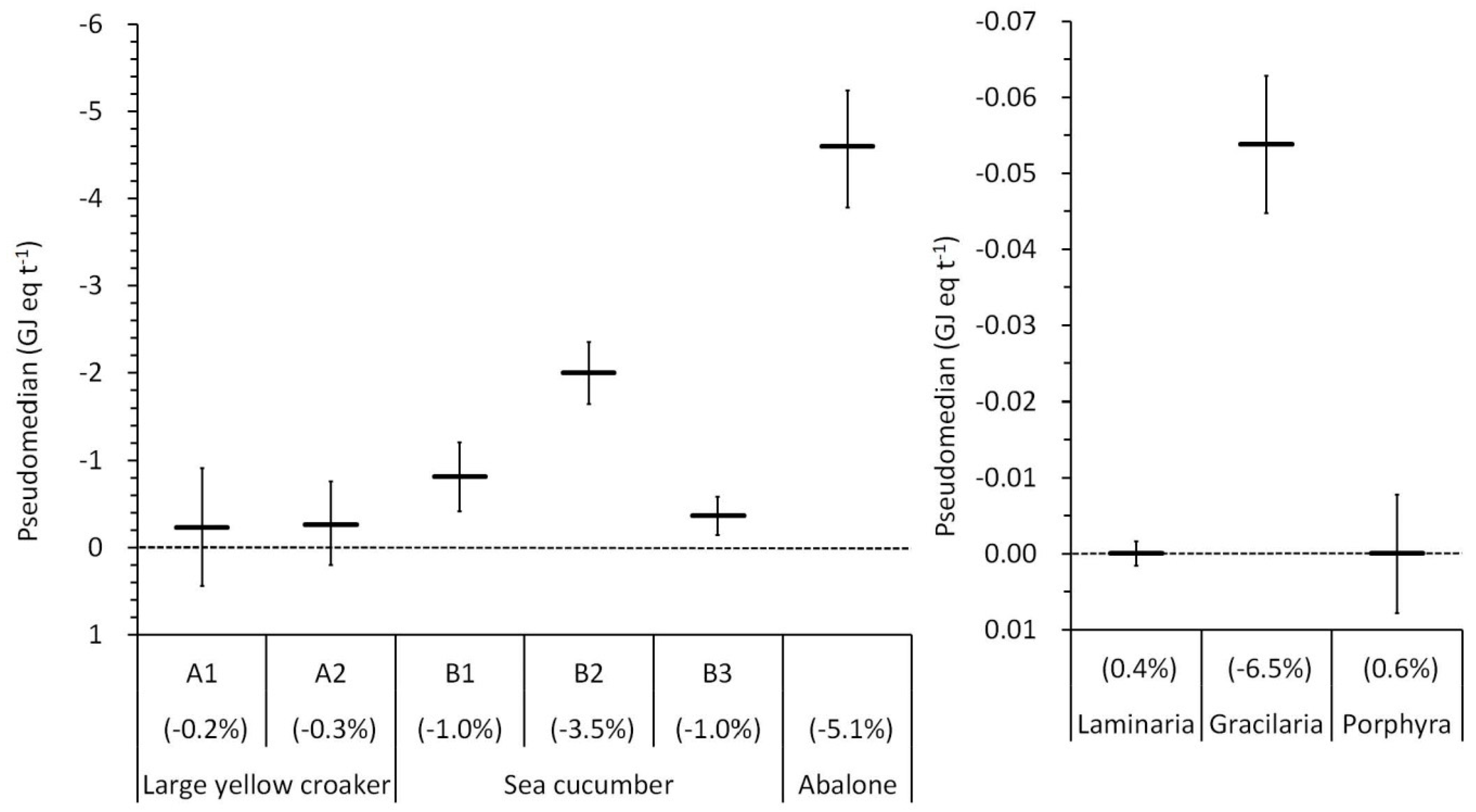
Figure 4.
Comparison between the standard error values of the total exergy demand obtained from the correlated and the uncorrelated model. The figure summarizes the results of the Wilcoxon signed-rank test and shows the estimate for the pseudomedian (horizontal line), the 99% confidence interval (whiskers), and the difference between the values from the correlated and uncorrelated models as a percentage value (x-axis, over the product label). The y-axis (pseudomedian) represents the difference of the standard error values between the correlated and uncorrelated models. For a description of the feed categories (A1-A2, B1-B3), see the footnote of Table 1.
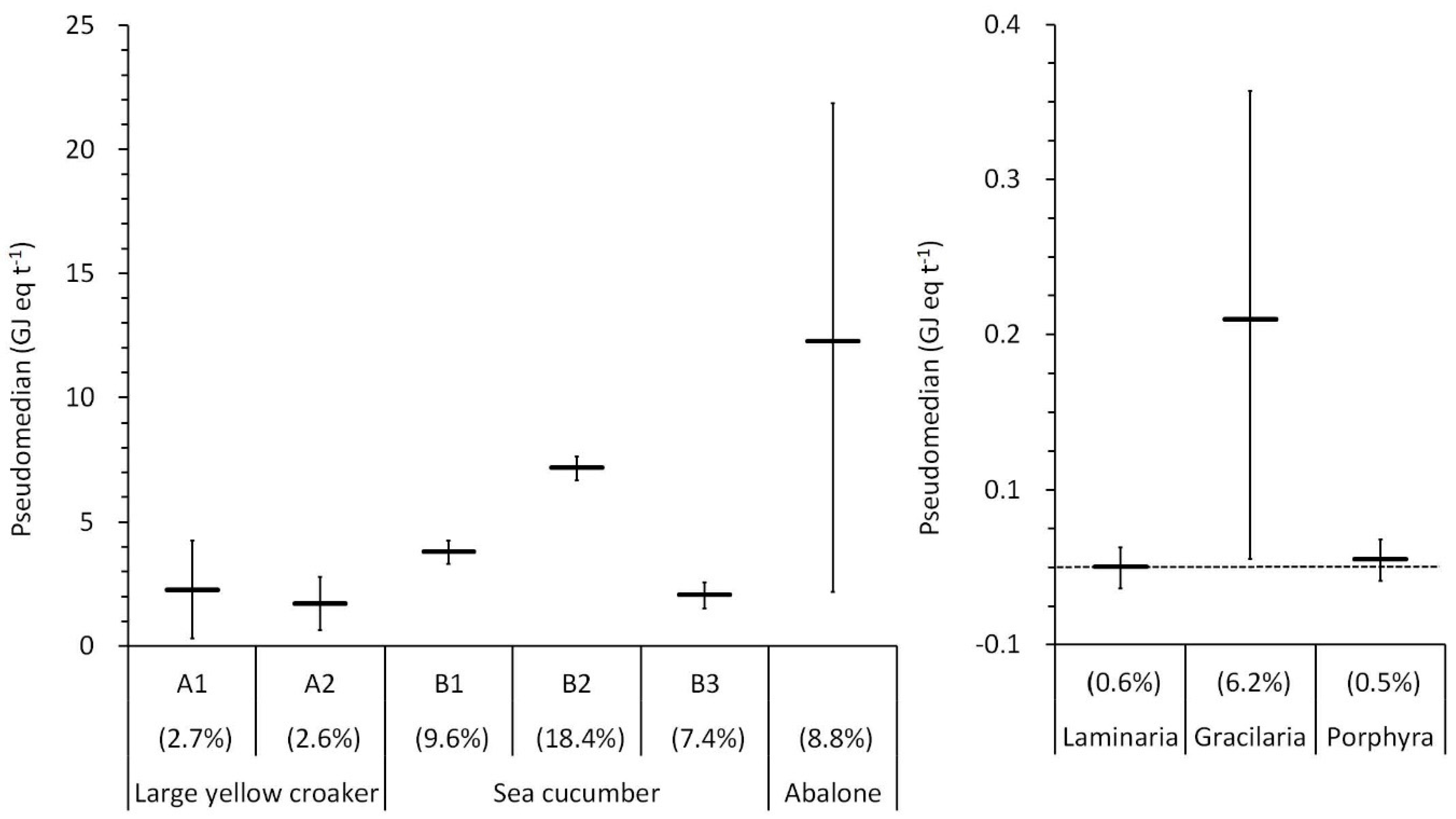
Figure 5.
Cumulated exergy demand of one live-weight ton of each product disaggregated by input contribution. The diagram shows the main stages of the production process (formulated feed, trash fish, and the main mariculture production chain), the inputs required in each stage and their respective contribution to the total exergy demand as a percentage value, and the locations of each unit process. (a) Large yellow croaker, abalone, and seaweed. (b) Sea cucumber. For a description of the feed categories (A1-A2, B1-B3), see the footnote in Table 1.

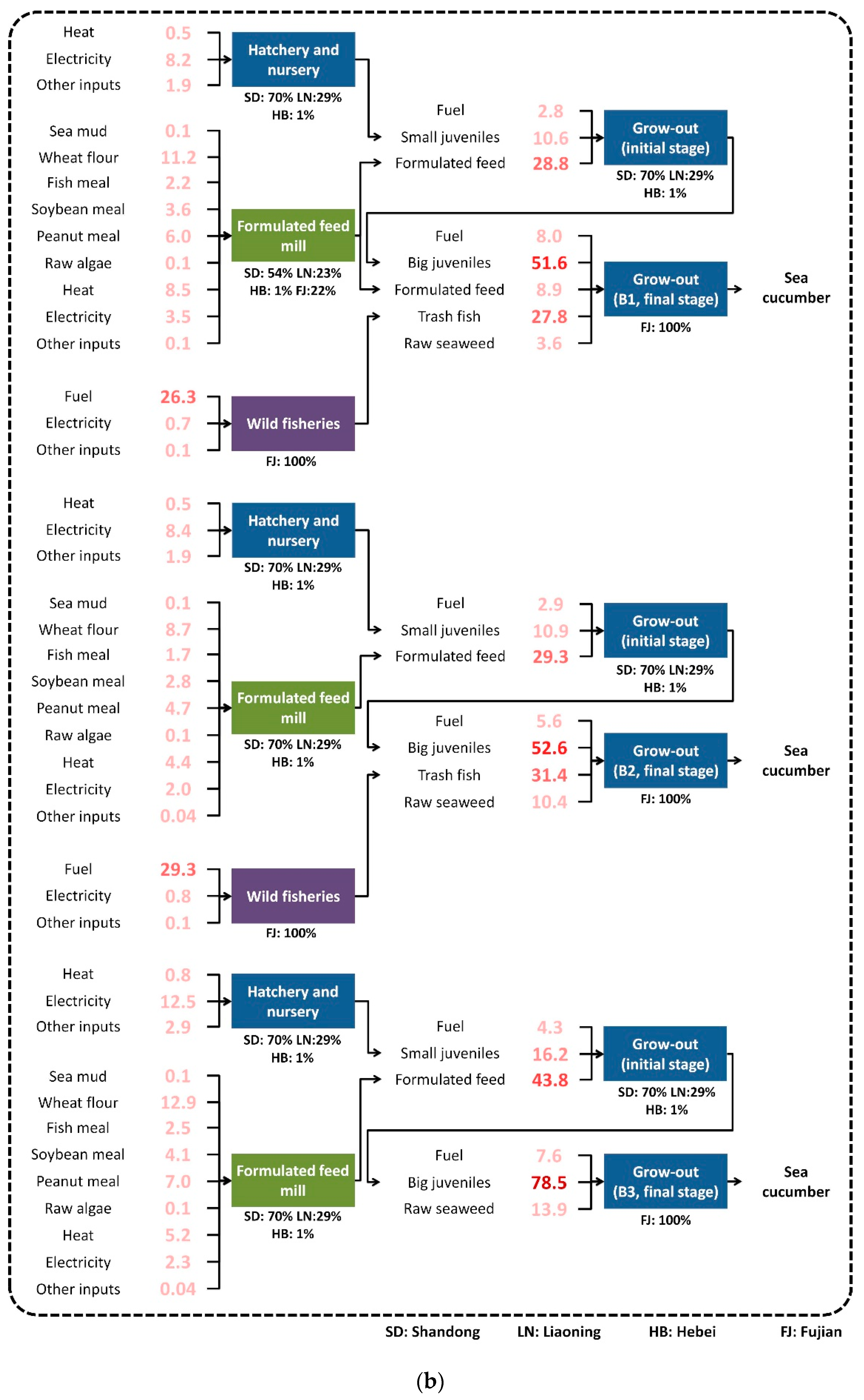
Figure 6.
Total exergy demand of one live-weight ton of each product. The boxes indicate the median, 25th and 75th percentiles, and the whiskers show the 90% confidence interval. For a description of the feed categories (A1-A2, B1-B3), see the footnote in Table 1.
Figure 6.
Total exergy demand of one live-weight ton of each product. The boxes indicate the median, 25th and 75th percentiles, and the whiskers show the 90% confidence interval. For a description of the feed categories (A1-A2, B1-B3), see the footnote in Table 1.
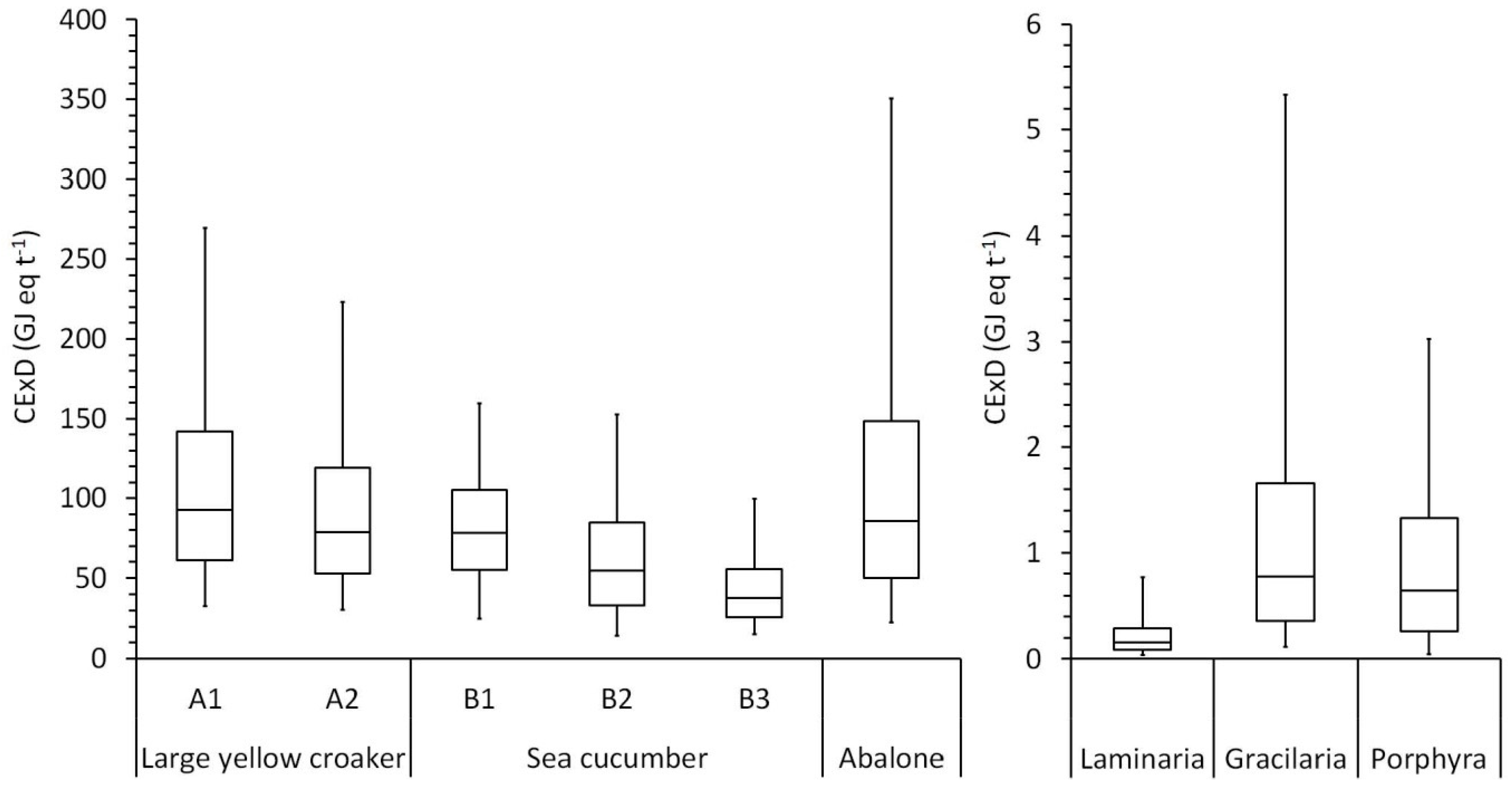
Figure 7.
Cumulated exergy demand (CExD) of one live-weight ton of each product by impact category based on the Ecoinvent database (v.3.5) [57]. The values show the contribution of each impact category of the CExD indicator to the total exergy demand as a percentage value. For a description of the feed categories (A1-A2, B1-B3), see the footnote in Table 1.

Figure 8.
Comparison between the total exergy demand values of different product categories. The figure summarizes the results of the Wilcoxon signed-rank test and shows the estimate for the pseudo-median (horizontal line) and the 99% confidence interval (whiskers). The labels indicate the categories that are being compared (e.g., A1-A2 is the difference in the total exergy demand between categories A1 and A2). For a description of the feed categories (A1-A2, B1-B3), see the footnote in Table 1.

Table 1.
Summary of the data collected in the survey.
| Product | Data Points (318 Households) | Product Proportion (292 Households) | Data Points Used in Modeling * |
|---|---|---|---|
| Large yellow croaker | 115 | 27.3 | 84 (A1); 18 (A2) |
| Sea cucumber | 44 | 10.5 | 10 (B1); 15 (B2); 11 (B3) |
| Abalone | 52 | 12.4 | 49 |
| Laminaria | 67 | 15.9 | 61 |
| Gracilaria | 61 | 14.5 | 61 |
| Porphyra | 39 | 9.3 | 36 |
| Other finfish | 43 | 10.1 | Not included |
| Other products ** | 57 | Not included | Not included |
Note: * Feed categories defined for animal products: A1: Formulated feed and trash fish; A2: Only trash fish; B1: Formulated feed, trash fish, and raw seaweed; B2: Trash fish and raw seaweed; B3: Only raw seaweed. ** This category includes non-finfish species, such as mudskipper, crab, oyster, razor clam, and shrimp.
Table 2.
Parameters of individual size (animal products) in each stage.
| Stage | Output | Large Yellow Croaker | Sea Cucumber | Abalone | |||
|---|---|---|---|---|---|---|---|
| Weight (g/unit) | Total Residence Time (months) | Weight (g/unit) | Total Residence Time (months) | Weight (g/unit) | Total Residence Time (months) | ||
| Hatchery/ nursery | Small juvenile | 0.39–2.16 * | 2 [50] | 0.20–2.50 [51,52] | 3 [51] | 0.04–1.21 [24,53] | 8 [54] |
| Initial grow-out (1) | Intermediate juvenile | - | - | 34.00–110.00 * [52] | 10 [55] | 2.10–5.00 * [24,53] | 12 [54] |
| Initial grow-out (2) | Big juvenile | - | - | - | - | 15.00–22.00 * [24,53] | 20 [54] |
| Final grow-out | Market-size product | 250.00–350.00 * [56] | 18 * | 138.00–169.00 * [52] | 16 * | 39.00–44.00 * [24,53] | 30 [54] |
Note: * Our survey data.
Table 3.
Life cycle inventory (median and coefficient of variation values) of the production of one live-weight ton of large yellow croaker, sea cucumber, and abalone. For a description of the feed categories (A1-A2, B1-B3), see the footnote in Table 1.
Table 3.
Life cycle inventory (median and coefficient of variation values) of the production of one live-weight ton of large yellow croaker, sea cucumber, and abalone. For a description of the feed categories (A1-A2, B1-B3), see the footnote in Table 1.
| Stage | Inputs/Outputs | Yellow Croaker | Sea Cucumber | Abalone | Unit | |||
|---|---|---|---|---|---|---|---|---|
| A1 | A2 | B1 | B2 | B3 | ||||
| Seed production inputs | Heat | 378.50 (1.49) | 486.70 (1.47) | 180.70 (1.62) | 118.20 (1.89) | 141.60 (1.68) | 681.50 (1.86) | MJ |
| Electricity | 287.20 (1.50) | 369.60 (1.47) | 402.00 (0.79) | 249.50 (1.04) | 288.60 (0.87) | 1386.20 (1.03) | kWh | |
| Fry feed | 1.10 (1.52) | 1.40 (1.49) | - | - | - | - | kg | |
| Liquid oxygen | 0.60 (1.53) | 0.80 (1.48) | 3.10 (0.84) | 1.90 (1.09) | 2.30 (0.92) | 10.80 (1.08) | kg | |
| Calcium carbonate | 11.10 (1.51) | 14.40 (1.50) | 57.10 (0.84) | 35.70 (1.09) | 41.40 (0.92) | 199.50 (1.08) | kg | |
| Chlorine | 0.01 (1.52) | 0.01 (1.50) | 0.04 (0.80) | 0.03 (1.04) | 0.03 (0.88) | 0.14 (1.04) | kg | |
| Intermediate inputs and exchanges | Juvenile transport to local farm | - | - | 2.70 (0.79) | 1.70 (1.04) | 2.00 (0.88) | 9.40 (1.03) | t km |
| Small juveniles | - | - | 14.20 (0.75) | 8.70 (0.99) | 10.10 (0.83) | 48.40 (0.99) | kg | |
| Initial grow-out inputs | Fuel | - | - | 18.60 (1.92) | 12.20 (2.17) | 14.60 (1.97) | 70.80 (2.05) | kg |
| Formulated feed | - | - | 1010.00 (0.63) | 618.00 (0.88) | 687.80 (0.72) | - | kg | |
| Raw seaweed (laminaria) | - | - | - | - | - | 1847.00 (1.10) | kg | |
| Raw seaweed (gracilaria) | - | - | - | - | - | 10842.90 (1.09) | kg | |
| Juvenile transport between farms (intermediate) | - | - | - | - | - | 633.30 (1.03) | t km | |
| Intermediate inputs and exchanges | Juvenile transport to Fujian province | - | - | 937.60 (0.72) | 585.10 (0.97) | 659.00 (0.80) | 378.70 (1.57) | t km |
| Juvenile transport to local farm | 0.50 (1.50) | 0.70 (1.47) | 105.20 (0.66) | 65.10 (0.91) | 72.90 (0.75) | 249.10 (0.78) | t km | |
| Big juveniles | 2.70 (1.46) | 3.50 (1.43) | 550.00 (0.61) | 335.40 (0.87) | 372.60 (0.70) | 1273.70 (0.73) | kg | |
| Final grow-out inputs | Fuel | 30.50 (0.78) | 33.60 (0.85) | 68.50 (1.29) | 41.60 (1.05) | 41.00 (1.00) | 58.50 (1.57) | kg |
| Formulated feed | 428.90 (1.59) | - | 280.20 (0.68) | - | - | - | kg | |
| Trash fish | 3588.40 (0.63) | 4197.90 (0.45) | 986.60 (0.84) | 889.50 (0.80) | - | - | kg | |
| Raw seaweed (laminaria) | - | - | 3097.00 (0.57) | 7041.00 (0.54) | 5130.50 (0.98) | 3154.20 (0.99) | kg | |
| Raw seaweed (gracilaria) | - | - | 753.40 (0.63) | 1714.90 (0.60) | 1258.10 (1.04) | 18627.10 (0.96) | kg | |
| Chemicals | 1.00 (2.05) | 0.40 (1.49) | - | - | - | - | kg | |
| System output parameters | Market-size product | 1.00 | 1.00 | 1.00 | 1.00 | 1.00 | 1.00 | t |
| Economic feed conversion ratio | 4.40 (0.58) | 4.20 (0.45) | 6.40 (0.50) | 10.60 (0.53) | 7.30 (0.91) | 38.80 (0.81) | - | |
Table 4.
Life cycle inventory (median and coefficient of variation values) of the production of one live-weight ton of laminaria, gracilaria, and porphyra.
Table 4.
Life cycle inventory (median and coefficient of variation values) of the production of one live-weight ton of laminaria, gracilaria, and porphyra.
| Stage | Inputs/Outputs | Laminaria | Gracilaria | Porphyra | Unit |
|---|---|---|---|---|---|
| Seed production inputs | Heat | 8.00 × 10⁻⁴ (0.80) | - | 1.22 × 10⁻² (0.31) | MJ |
| Electricity | 4.00 × 10⁻⁴ (0.80) | - | 6.60 × 10⁻³ (0.31) | kWh | |
| Intermediate inputs and exchanges | Seed transport to Fujian province | - | - | 0.87 (0.28) | t km |
| Seed transport to local farm | 0.01 (0.72) | - | 0.20 (0.21) | t km | |
| Seeds | 0.06 (0.70) | 145.32 (1.96) | 2.46 (0.85) | kg | |
| Grow-out inputs | Fuel | 2.32 (1.38) | 9.47 (2.01) | 10.92 (1.07) | kg |
| Chemicals | 0.01 (0.53) | - | - | kg | |
| System output parameters | Market-size product | 1.00 | 1.00 | 1.00 | t |
© 2019 by the authors. Licensee MDPI, Basel, Switzerland. This article is an open access article distributed under the terms and conditions of the Creative Commons Attribution (CC BY) license (http://creativecommons.org/licenses/by/4.0/).
Share and Cite
MDPI and ACS Style
Marín, T.; Wu, J.; Wu, X.; Ying, Z.; Lu, Q.; Hong, Y.; Wang, X.; Yang, W. Resource Use in Mariculture: A Case Study in Southeastern China. Sustainability 2019, 11, 1396. https://doi.org/10.3390/su11051396
AMA Style
Marín T, Wu J, Wu X, Ying Z, Lu Q, Hong Y, Wang X, Yang W. Resource Use in Mariculture: A Case Study in Southeastern China. Sustainability. 2019; 11(5):1396. https://doi.org/10.3390/su11051396
Chicago/Turabian StyleMarín, Tomás, Jing Wu, Xu Wu, Zimin Ying, Qiaoling Lu, Yiyuan Hong, Xiaoyan Wang, and Wu Yang. 2019. "Resource Use in Mariculture: A Case Study in Southeastern China" Sustainability 11, no. 5: 1396. https://doi.org/10.3390/su11051396
Note that from the first issue of 2016, this journal uses article numbers instead of page numbers. See further details here.