Prioritizing Spatially Aggregated Cost-Effective Sites in Natural Reserves to Mitigate Human-Induced Threats: A Case Study of the Qinghai Plateau, China

Abstract
:1. Introduction
2. Materials and Methods
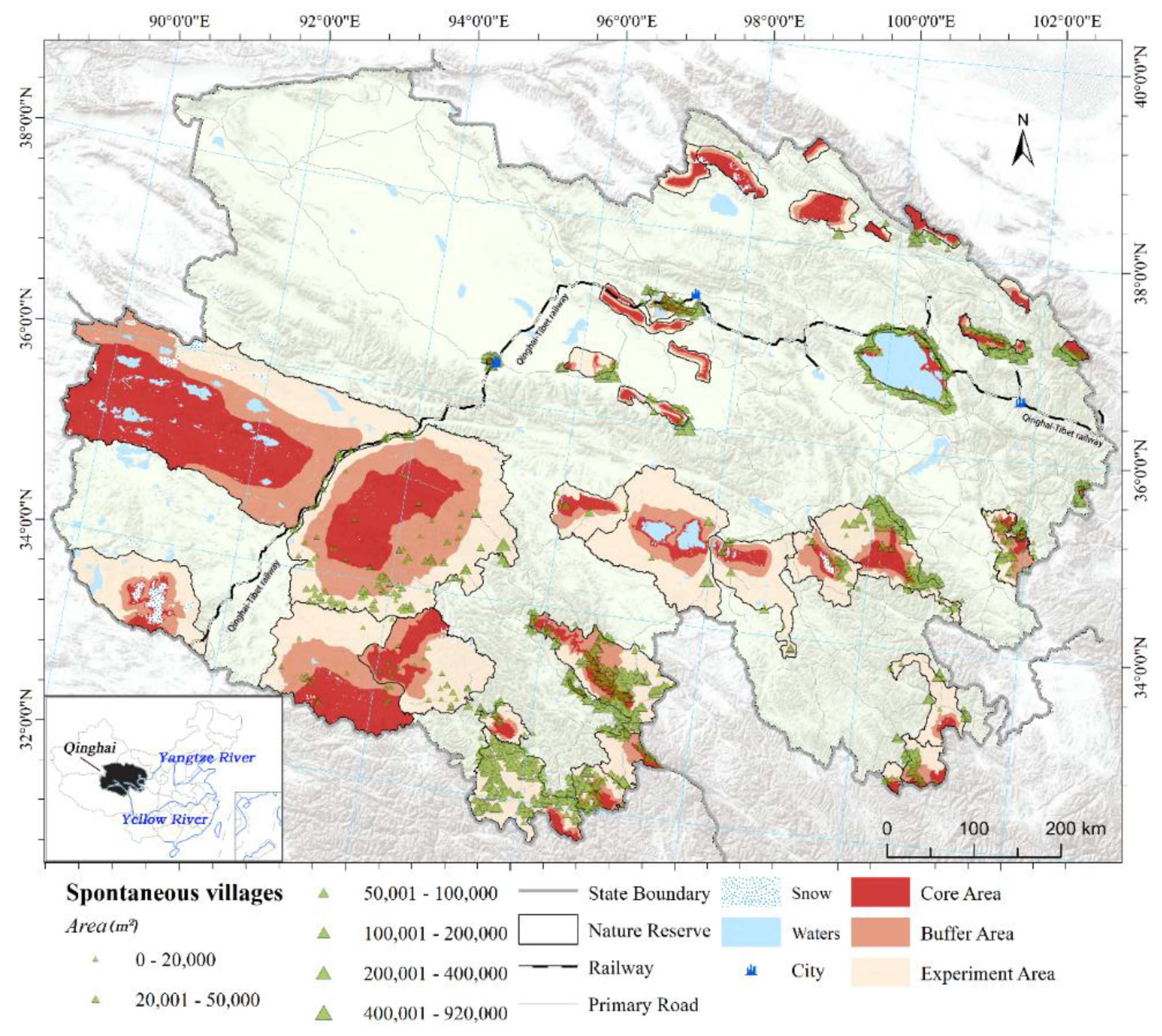
2.1. Study Area
2.2. Materials
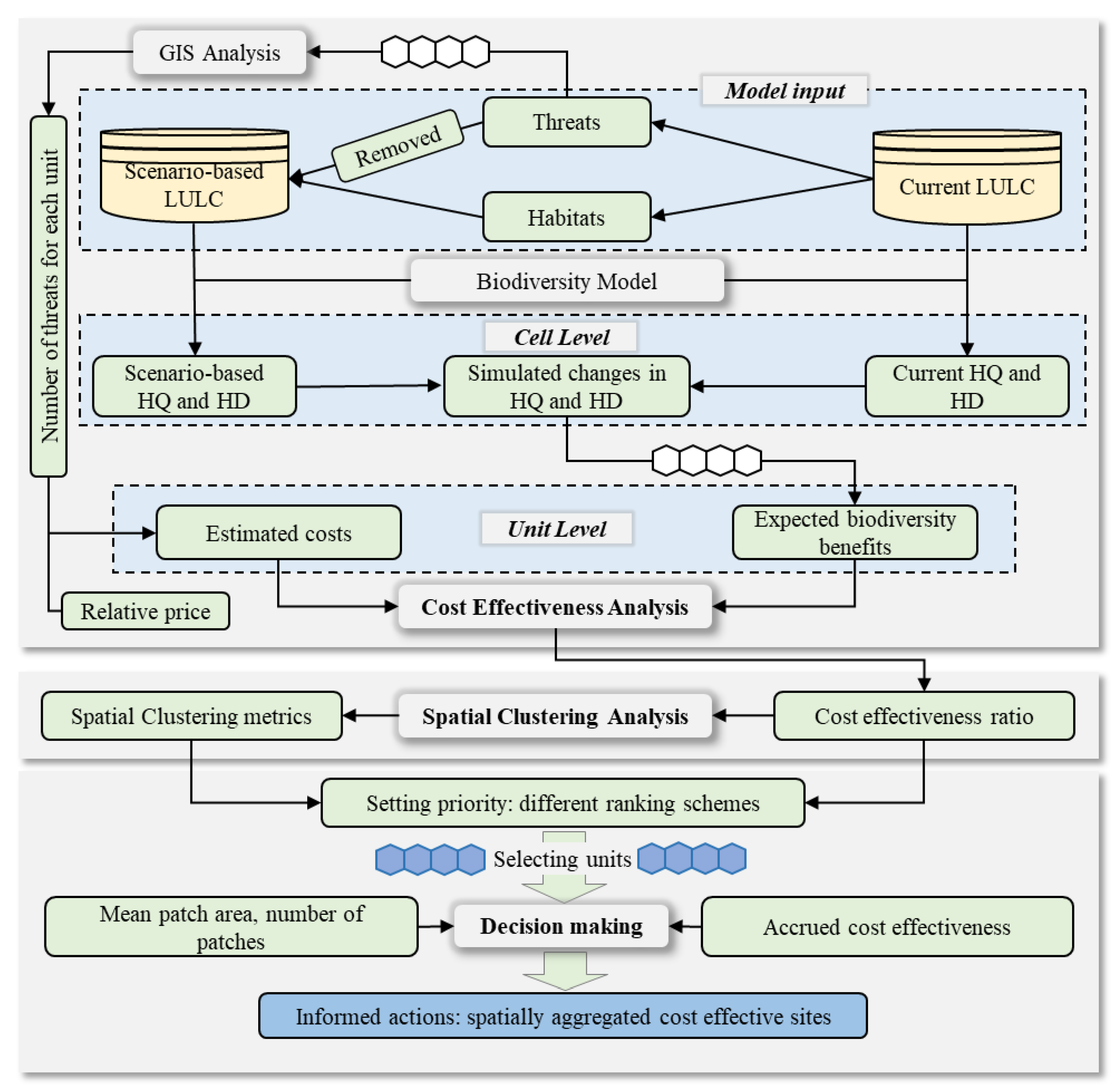
2.3. Methods
2.3.1. Cost Effectiveness Analysis
- Evaluation of expected biodiversity benefits
- Estimation of threat management costs
- Calculation of cost effectiveness ratio
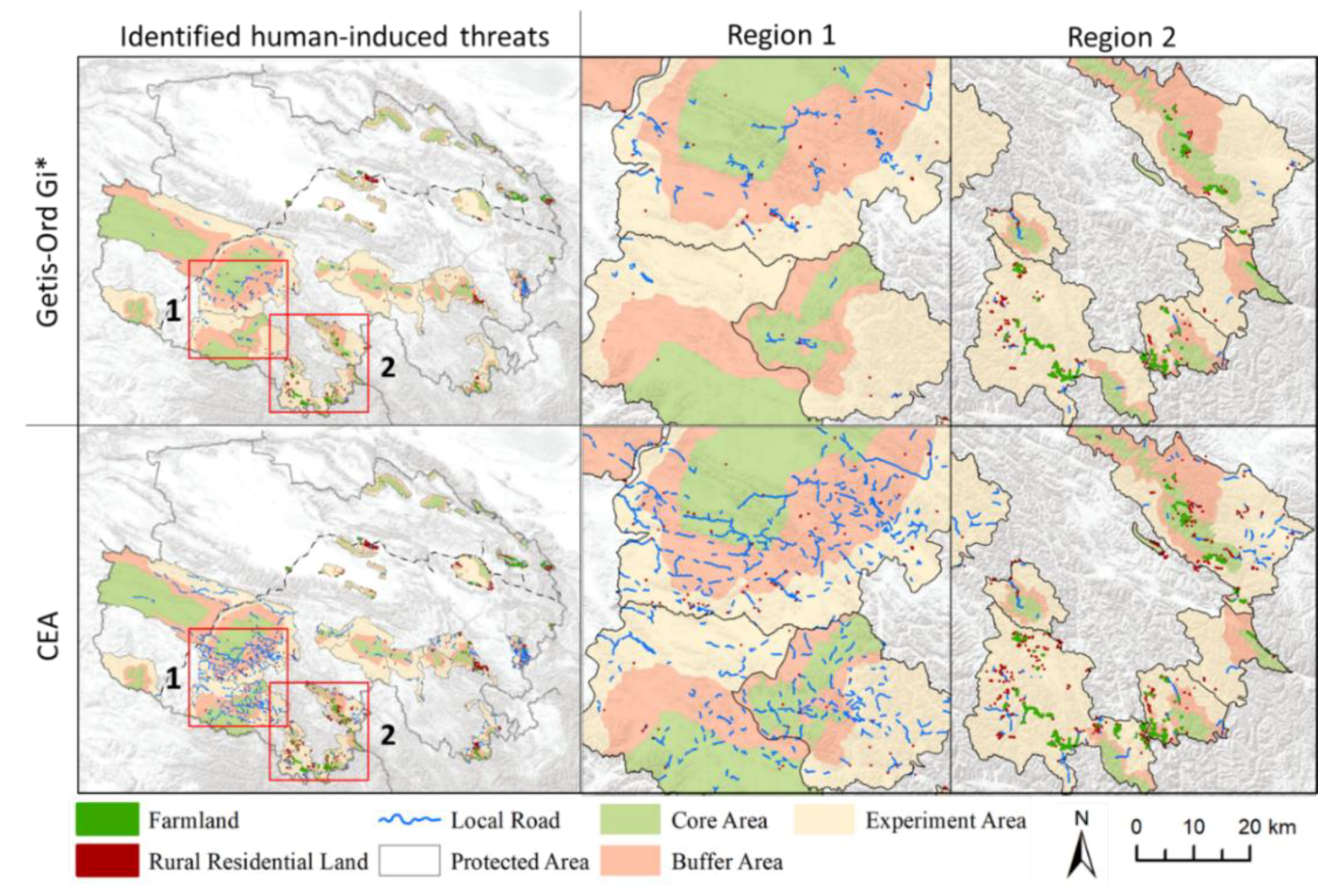
2.3.2. Identifying Spatially Clustered Sites for Threat Management
2.3.3. Priority Setting
2.3.4. Comparison with Traditional Prioritization Index
3. Results
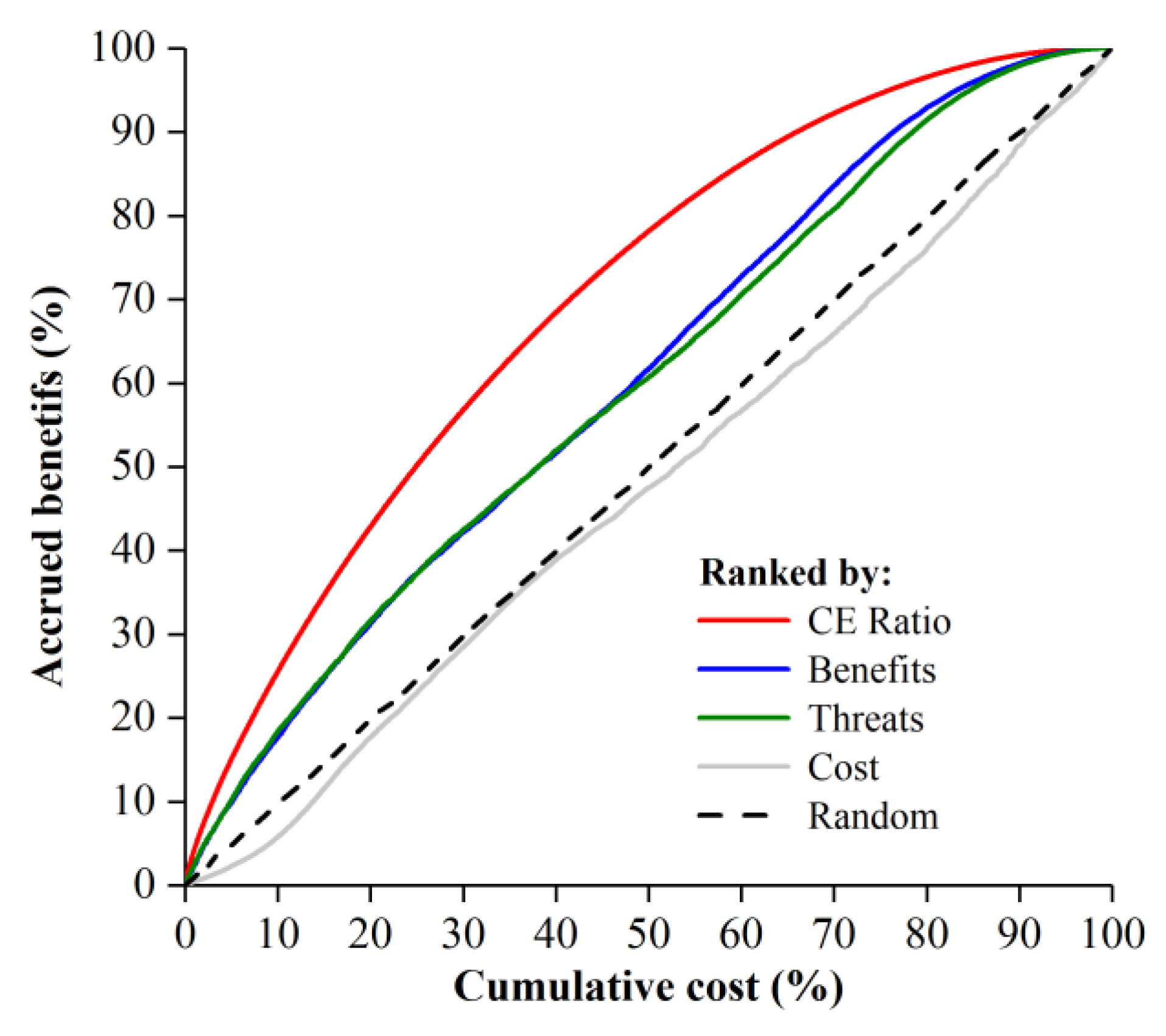
3.1. Cost Effectiveness of Units Prioritized by CEA and Traditional Index
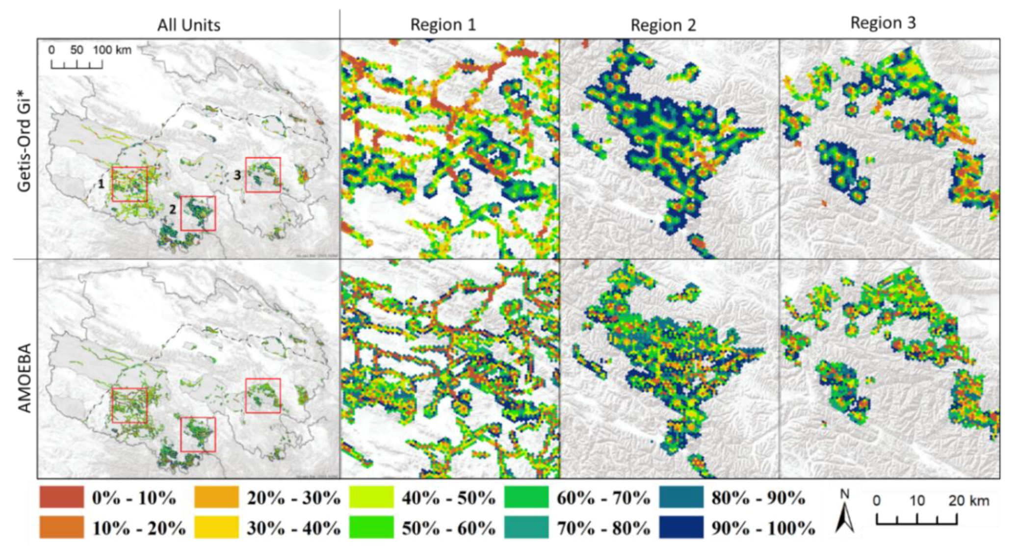
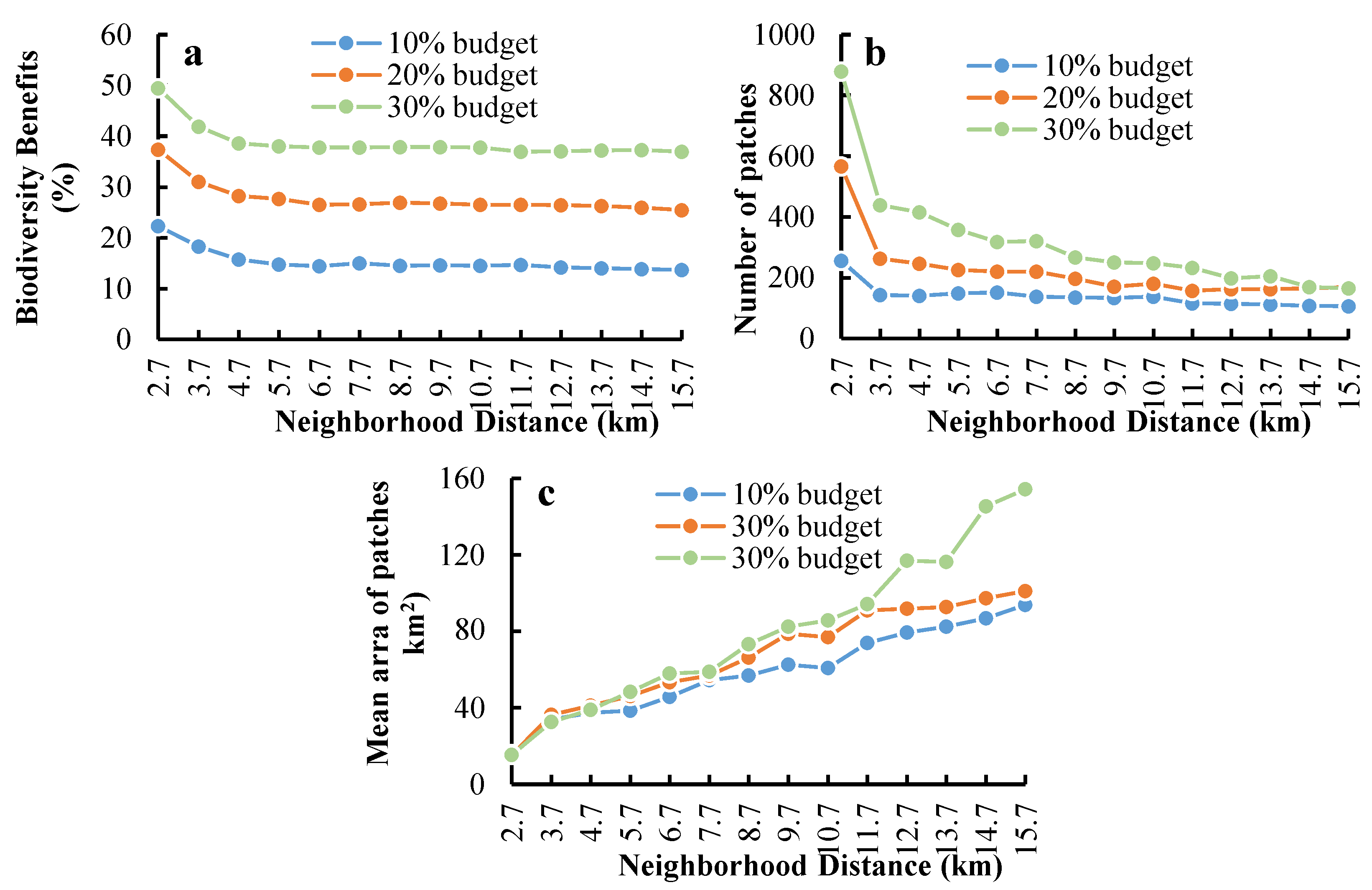
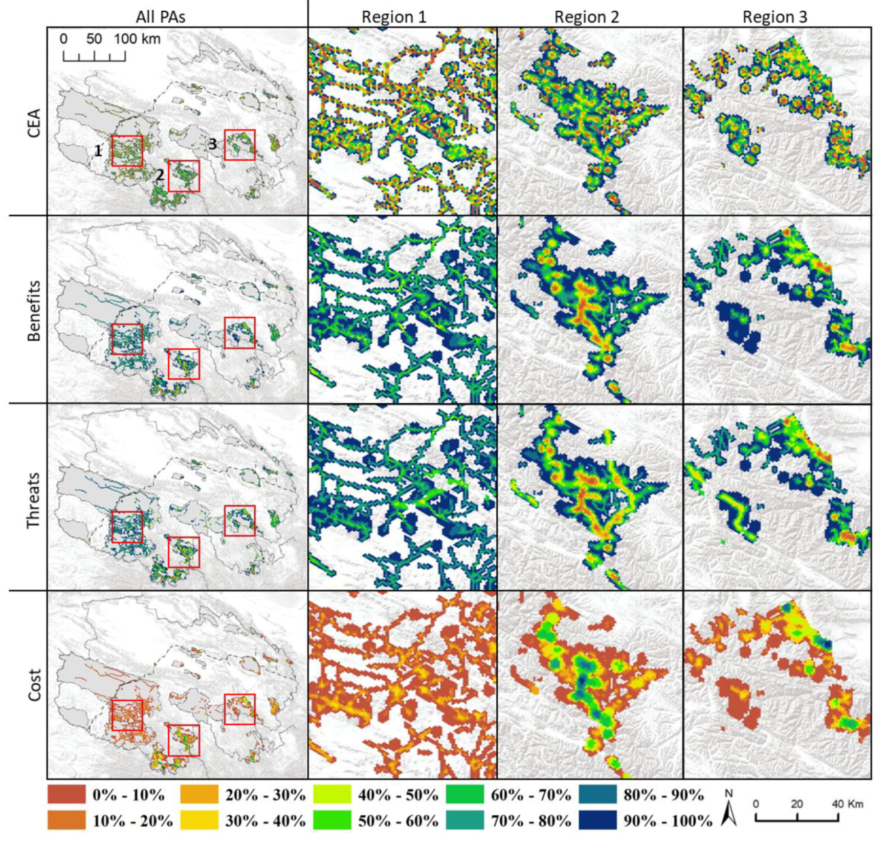
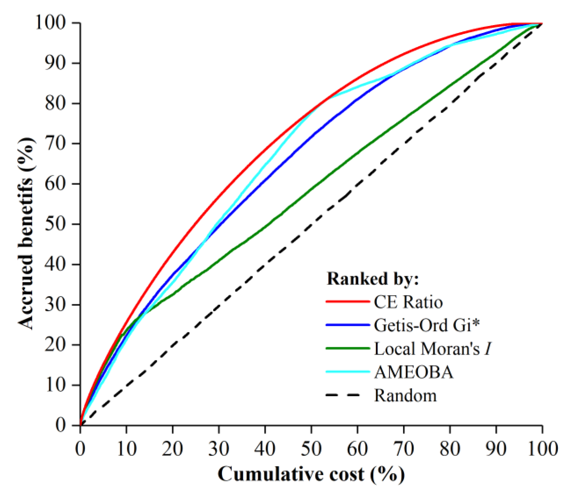
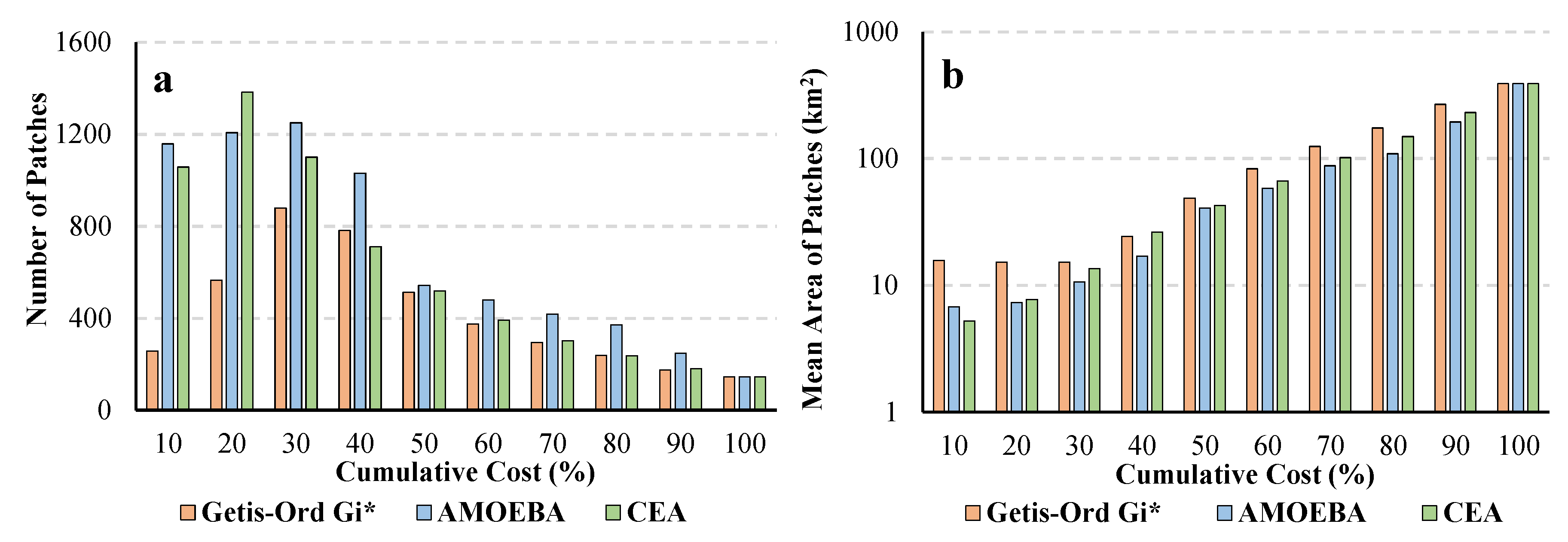
3.2. Spatial Aggregation and Cost Effectiveness of Units Prioritized by Spatial Clustering Statistics
3.3. Actual Costs of Units Identified by Spatial Clustering Statistics
4. Discussion
4.1. Feasibility of the CEA Method
4.2. Spatial Clustering Statistics Identify Spatially Aggregated Cost-Effective Sites
4.3. Differences between Sites from Alternative Spatial Clustering Statistics
5. Conclusions
Supplementary Materials
Author Contributions
Funding
Acknowledgments
Conflicts of Interest
References
- Cegielska, K.; Kukulska-Kozieł, A.; Salata, T.; Piotrowski, P.; Szylar, M. Shannon entropy as a peri-urban landscape metric: Concentration of anthropogenic land cover element. J. Sp. Sci. 2018. [Google Scholar] [CrossRef]
- Noszczyk, T.; Rutkowska, A.; Hernik, J. Exploring the land use changes in Eastern Poland: Statistics-based modeling. Hum. Ecol. Risk Assess. Int. J. 2019. [Google Scholar] [CrossRef]
- Newbold, T.; Hudson, L.N.; Arnell, A.P.; Contu, S.; De Palma, A.; Ferrier, S.; Hill, S.L.; Hoskins, A.J.; Lysenko, I.; Phillips, H.R. Has land use pushed terrestrial biodiversity beyond the planetary boundary? A global assessment. Science 2016, 353, 288–291. [Google Scholar] [CrossRef] [PubMed] [Green Version]
- Bartula, M.; Stojšić, V.; Perić, R.; Kitnæs, K.S. Protection of Natura 2000 habitat types in the Ramsar Site “Zasavica Special Nature Reserve” in Serbia. Nat. Areas J. 2011, 31, 349–357. [Google Scholar] [CrossRef]
- Run, S.; Shuangling, W.; Linqiao, W.; Hui, A.; Shiying, Q.; Youjun, L.; Weifu, T. How to balance development between nature reserves and community: A case study in Shiwandashan National Nature Reserve, Guangxi. Biodivers. Sci. 2017, 25, 437–448. [Google Scholar]
- Hobbs, R.J.; Norton, D.A. Towards a conceptual framework for restoration ecology. Restor. Ecol. 1996, 4, 93–110. [Google Scholar] [CrossRef]
- Margules, C.; Sarkar, S. Systematic Conservation Planning; Cambridge University Press: Cambridge, UK, 2007. [Google Scholar]
- Kimball, S.; Lulow, M.; Sorenson, Q.; Balazs, K.; Fang, Y.-C.; Davis, S.J.; O’Connell, M.; Huxman, T.E. Cost-effective ecological restoration. Restor. Ecol. 2015, 23, 800–810. [Google Scholar] [CrossRef] [Green Version]
- Knight, A.T.; Cowling, R.M.; Rouget, M.; Balmford, A.; Lombard, A.T.; Campbell, B.M. Knowing but not doing: Selecting priority conservation areas and the research-implementation gap. Conserv. Biol. 2008, 22, 610–617. [Google Scholar] [CrossRef] [PubMed]
- Carwardine, J.; O’Connor, T.; Legge, S.; Mackey, B.; Possingham, H.P.; Martin, T.G. Prioritizing threat management for biodiversity conservation. Conserv. Lett. 2012, 5, 196–204. [Google Scholar] [CrossRef] [Green Version]
- Tulloch, V.J.D.; Tulloch, A.I.T.; Visconti, P.; Halpern, B.S.; Watson, J.E.M.; Evans, M.C.; Auerbach, N.A.; Barnes, M.; Beger, M.; Chadès, I.; et al. Why do we map threats? Linking threat mapping with actions to make better conservation decisions. Front. Ecol. Environ. 2015, 13, 91–99. [Google Scholar] [CrossRef] [Green Version]
- Naidoo, R.; Balmford, A.; Ferraro, P.J.; Polasky, S.; Ricketts, T.H.; Rouget, M. Integrating economic costs into conservation planning. Trends Ecol. Evol. 2006, 21, 681–687. [Google Scholar] [CrossRef] [PubMed]
- Tear, T.H.; Stratton, B.N.; Game, E.T.; Brown, M.A.; Apse, C.D.; Shirer, R.R. A return-on-investment framework to identify conservation priorities in Africa. Biol. Conserv. 2014, 173, 42–52. [Google Scholar] [CrossRef] [Green Version]
- Murdoch, W.; Polasky, S.; Wilson, K.A.; Possingham, H.P.; Kareiva, P.; Shaw, R. Maximizing return on investment in conservation. Biol. Conserv. 2007, 139, 375–388. [Google Scholar] [CrossRef]
- Donlan, C.J.; Luque, G.M.; Wilcox, C. Maximizing return on investment for island restoration and species conservation. Conserv. Lett. 2015, 8, 171–179. [Google Scholar] [CrossRef]
- Bottrill, M.C.; Joseph, L.N.; Carwardine, J.; Bode, M.; Cook, C.; Game, E.T.; Grantham, H.; Kark, S.; Linke, S.; McDonald-Madden, E. Is conservation triage just smart decision making? Trends Ecol. Evol. 2008, 23, 649–654. [Google Scholar] [CrossRef] [PubMed]
- Balana, B.B.; Vinten, A.; Slee, B. A review on cost-effectiveness analysis of agri-environmental measures related to the EU WFD: Key issues, methods, and applications. Ecol. Econ. 2011, 70, 1021–1031. [Google Scholar] [CrossRef]
- Weinstein, M.C.; Stason, W.B. Foundations of cost-effectiveness analysis for health and medical practices. N. Engl. J. Med. 1977, 296, 716–721. [Google Scholar] [CrossRef] [PubMed]
- Gren, I.-M.; Baxter, P.; Mikusinski, G.; Possingham, H. Cost-effective biodiversity restoration with uncertain growth in forest habitat quality. J. For. Econ. 2014, 20, 77–92. [Google Scholar] [CrossRef]
- Underwood, E.C.; Shaw, M.R.; Wilson, K.A.; Kareiva, P.; Klausmeyer, K.R.; McBride, M.F.; Bode, M.; Morrison, S.A.; Hoekstra, J.M.; Possingham, H.P. Protecting biodiversity when money matters: Maximizing return on investment. PLoS ONE 2008, 3, e1515. [Google Scholar] [CrossRef] [PubMed]
- Arponen, A.; Cabeza, M.; Eklund, J.; Kujala, H.; Lehtomaeki, J. Costs of integrating economics and conservation planning. Conserv. Biol. 2010, 24, 1198–1204. [Google Scholar] [CrossRef] [PubMed]
- Boyd, J.; Epanchin-Niell, R.; Siikamäki, J. Conservation return on investment analysis: A review of results, methods, and new directions. Resources for the Future Discussion Paper, 10 January 2012. [Google Scholar]
- Kramer, D.B.; Zhang, T.; Cheruvelil, K.S.; Ligmann-Zielinska, A.; Soranno, P.A. A multi-objective, return on investment analysis for freshwater conservation planning. Ecosystems 2013, 16, 823–837. [Google Scholar] [CrossRef]
- Auerbach, N.A.; Tulloch, A.I.T.; Possingham, H.P. Informed actions: Where to cost effectively manage multiple threats to species to maximize return on investment. Ecol. Appl. 2014, 24, 1357–1373. [Google Scholar] [CrossRef] [PubMed]
- Murdoch, W.; Ranganathan, J.; Polasky, S.; Regetz, J. Using return on investment to maximize conservation effectiveness in Argentine grasslands. Proc. Natl. Acad. Sci. USA 2010, 107, 20855–20862. [Google Scholar] [CrossRef] [PubMed] [Green Version]
- Kovacs, K.; Polasky, S.; Nelson, E.; Keeler, B.L.; Pennington, D.; Plantinga, A.J.; Taff, S.J. Evaluating the return in ecosystem services from investment in public land acquisitions. PLoS ONE 2013, 8, e62202. [Google Scholar] [CrossRef] [PubMed]
- Di Minin, E.; Soutullo, A.; Bartesaghi, L.; Rios, M.; Szephegyi, M.N.; Moilanen, A. Integrating biodiversity, ecosystem services and socio-economic data to identify priority areas and landowners for conservation actions at the national scale. Biol. Conserv. 2017, 206, 56–64. [Google Scholar] [CrossRef]
- Lewis, D.J.; Plantinga, A.J.; Nelson, E.; Polasky, S. The efficiency of voluntary incentive policies for preventing biodiversity loss. Resour. Energy Econ. 2011, 33, 192–211. [Google Scholar] [CrossRef] [Green Version]
- Joseph, L.N.; Maloney, R.F.; Possingham, H.P. Optimal allocation of resources among threatened species: A project prioritization protocol. Conserv. Biol. 2009, 23, 328–338. [Google Scholar] [CrossRef] [PubMed]
- Cullen, R.; White, P.C. Prioritising and evaluating biodiversity projects. Wildl. Res. 2013, 40, 91–93. [Google Scholar] [CrossRef] [Green Version]
- Williams, J.C.; ReVelle, C.S.; Levin, S.A. Spatial attributes and reserve design models: A review. Environ. Model. Assess. 2005, 10, 163–181. [Google Scholar] [CrossRef]
- Wilson, K.A.; Lulow, M.; Burger, J.; Fang, Y.-C.; Andersen, C.; Olson, D.; O’Connell, M.; McBride, M.F. Optimal restoration: Accounting for space, time and uncertainty. J. Appl. Ecol. 2011, 48, 715–725. [Google Scholar] [CrossRef]
- Auerbach, N.A.; Wilson, K.A.; Tulloch, A.I.; Rhodes, J.R.; Hanson, J.O.; Possingham, H.P. Effects of threat management interactions on conservation priorities. Conserv. Biol. 2015, 29, 1626–1635. [Google Scholar] [CrossRef] [PubMed] [Green Version]
- Kukkala, A.S.; Moilanen, A. Core concepts of spatial prioritisation in systematic conservation planning. Biol. Rev. 2013, 88, 443–464. [Google Scholar] [CrossRef] [PubMed]
- Brudvig, L.A.; Damschen, E.I.; Tewksbury, J.J.; Haddad, N.M.; Levey, D.J. Landscape connectivity promotes plant biodiversity spillover into non-target habitats. Proc. Natl. Acad. Sci. USA 2009, 106, 9328–9332. [Google Scholar] [CrossRef] [PubMed] [Green Version]
- Blitzer, E.J.; Dormann, C.F.; Holzschuh, A.; Klein, A.-M.; Rand, T.A.; Tscharntke, T. Spillover of functionally important organisms between managed and natural habitats. Agric. Ecosyst. Environ. 2012, 146, 34–43. [Google Scholar] [CrossRef] [Green Version]
- Wan, G.H.; Cheng, E.J. Effects of land fragmentation and returns to scale in the Chinese farming sector. Appl. Econ. 2001, 33, 183–194. [Google Scholar] [CrossRef]
- Drechsler, M.; Watzold, F.; Johst, K.; Shogren, J.F. An agglomeration payment for cost-effective biodiversity conservation in spatially structured landscapes. Resour. Energy Econ. 2010, 32, 261–275. [Google Scholar] [CrossRef] [Green Version]
- Hanley, N.; Banerjee, S.; Lennox, G.D.; Armsworth, P.R. How should we incentivize private landowners to ‘produce’more biodiversity? Oxf. Review Econ. Policy 2012, 28, 93–113. [Google Scholar] [CrossRef]
- Forman, R. Land Mosaics: The Ecology of Landscapes and Regions 1995; Island Press: Washington, DC, USA, 2014. [Google Scholar]
- Jongman, R.H.; Külvik, M.; Kristiansen, I. European ecological networks and greenways. Landsc. Urban Plan. 2004, 68, 305–319. [Google Scholar] [CrossRef]
- BenDor, T.K.; Spurlock, D.; Woodruff, S.C.; Olander, L. A research agenda for ecosystem services in American environmental and land use planning. Cities 2017, 60, 260–271. [Google Scholar] [CrossRef]
- Armsworth, P.R.; Cantu-Salazar, L.; Parnell, M.; Davies, Z.G.; Stoneman, R. Management costs for small protected areas and economies of scale in habitat conservation. Biol. Conserv. 2011, 144, 423–429. [Google Scholar] [CrossRef] [Green Version]
- Lawley, C.; Yang, W.H. Spatial interactions in habitat conservation: Evidence from prairie pothole easements. J. Environ. Econ. Manag. 2015, 71, 71–89. [Google Scholar] [CrossRef]
- Ndubisi, F.O. The Ecological Design and Planning Reader; Island Press: Washington, DC, USA, 2014. [Google Scholar]
- Boyd, J.; Epanchin-Niell, R.; Siikamäki, J. Conservation planning: A review of return on investment analysis. Rev. Environ. Econ. Policy 2015, 9, 23–42. [Google Scholar] [CrossRef]
- Ball, I.R.; Possingham, H.P.; Watts, M. Marxan and relatives: Software for spatial conservation prioritisation. In Spatial Conservation Prioritization: Quantitative Methods and Computational Tools; Cambridge University Press: Cambridge, UK, 2009; Volume 14, pp. 185–195. [Google Scholar]
- Liu, Y.L.; Peng, J.J.; Jiao, L.M.; Liu, Y.F. PSOLA: A Heuristic Land-Use Allocation Model Using Patch-Level Operations and Knowledge-Informed Rules. PLoS ONE 2016, 11, e0157728. [Google Scholar] [CrossRef] [PubMed]
- Liu, D.; Tang, W.; Liu, Y.; Zhao, X.; He, J. Optimal rural land use allocation in central China: Linking the effect of spatiotemporal patterns and policy interventions. Appl. Geogr. 2017, 86, 165–182. [Google Scholar] [CrossRef]
- Kaim, A.; Cord, A.F.; Volk, M. A review of multi-criteria optimization techniques for agricultural land use allocation. Environ. Model. Softw. 2018, 105, 79–93. [Google Scholar] [CrossRef]
- Schröter, M.; Remme, R.P. Spatial prioritisation for conserving ecosystem services: Comparing hotspots with heuristic optimisation. Landsc. Ecol. 2016, 31, 431–450. [Google Scholar] [CrossRef] [PubMed]
- Possingham, H.; Ball, I.; Andelman, S. Mathematical Methods for Identifying Representative Reserve Networks. In Quantitative Methods for Conservation Biology; Springer: New York, NY, USA, 2000; pp. 291–306. [Google Scholar]
- Anselin, L. Local indicators of spatial association—LISA. Geogr. Anal. 1995, 27, 93–115. [Google Scholar] [CrossRef]
- Getis, A.; Ord, J.K. The analysis of spatial association by use of distance statistics. Geogr. Anal. 1992, 24, 189–206. [Google Scholar] [CrossRef]
- Bagstad, K.J.; Reed, J.M.; Semmens, D.J.; Sherrouse, B.C.; Troy, A. Linking biophysical models and public preferences for ecosystem service assessments: A case study for the Southern Rocky Mountains. Reg. Environ. Chang. 2016, 16, 2005–2018. [Google Scholar] [CrossRef]
- Sallustio, L.; De Toni, A.; Strollo, A.; Di Febbraro, M.; Gissi, E.; Casella, L.; Geneletti, D.; Munafo, M.; Vizzarri, M.; Marchetti, M. Assessing habitat quality in relation to the spatial distribution of protected areas in Italy. J. Environ. Manag. 2017, 201, 129–137. [Google Scholar] [CrossRef] [PubMed]
- Grubesic, T.H.; Wei, R.; Murray, A.T. Spatial clustering overview and comparison: Accuracy, sensitivity, and computational expense. Ann. Assoc. Am. Geogr. 2014, 104, 1134–1156. [Google Scholar] [CrossRef]
- Xu, X.; Lu, C.; Shi, X.; Gao, S. World water tower: An atmospheric perspective. Geophys. Res. Lett. 2008, 35. [Google Scholar] [CrossRef] [Green Version]
- Myers, N.; Mittermeier, R.A.; Mittermeier, C.G.; Da Fonseca, G.A.; Kent, J. Biodiversity hotspots for conservation priorities. Nature 2000, 403, 853–858. [Google Scholar] [CrossRef] [PubMed]
- Le Saout, S.; Hoffmann, M.; Shi, Y.; Hughes, A.; Bernard, C.; Brooks, T.M.; Bertzky, B.; Butchart, S.H.; Stuart, S.N.; Badman, T.; et al. Protected areas and effective biodiversity conservation. Science 2013, 342, 803–805. [Google Scholar] [CrossRef] [PubMed]
- Hull, V.; Xu, W.; Liu, W.; Zhou, S.; Viña, A.; Zhang, J.; Tuanmu, M.-N.; Huang, J.; Linderman, M.; Chen, X. Evaluating the efficacy of zoning designations for protected area management. Biol. Conserv. 2011, 144, 3028–3037. [Google Scholar] [CrossRef] [Green Version]
- Li, X.-l.; Brierley, G.; Shi, D.-j.; Xie, Y.-l.; Sun, H.-q. Ecological protection and restoration in Sanjiangyuan national nature reserve, Qinghai Province, China. In Perspectives on Environmental Management and Technology in Asian River Basins; Springer: Dordrecht, The Netherlands, 2012; pp. 93–120. [Google Scholar]
- Chen, H.; Zhu, Q.; Peng, C.; Wu, N.; Wang, Y.; Fang, X.; Gao, Y.; Zhu, D.; Yang, G.; Tian, J. The impacts of climate change and human activities on biogeochemical cycles on the Qinghai-Tibetan Plateau. Glob. Chang. Biol. 2013, 19, 2940–2955. [Google Scholar] [CrossRef] [PubMed] [Green Version]
- Li, S.; Zhang, Y.; Wang, Z.; Li, L. Mapping human influence intensity in the Tibetan Plateau for conservation of ecological service functions. Ecosyst. Serv. 2018, 30, 276–286. [Google Scholar] [CrossRef]
- Yao, T.; Thompson, L.G.; Mosbrugger, V.; Zhang, F.; Ma, Y.; Luo, T.; Xu, B.; Yang, X.; Joswiak, D.R.; Wang, W. Third pole environment (TPE). Environ. Dev. 2012, 3, 52–64. [Google Scholar] [CrossRef]
- United Nations Development Programme—Global Environmental Finance Unit. Strengthening the Effectiveness of the Protected Area System in Qinghai Province; UNDP: New York, NY, USA, 2013. [Google Scholar]
- Shao, Q.; Fan, J.; Liu, J.; Huang, L.; Cao, W.; Xu, X.; Ge, J.; Wu, D.; Li, Z.; Gong, G. Assessment on the effects of the first-stage ecological conservation and restoration project in Sanjiangyuan region. Acta Geogr. Sin. 2016, 71, 3–20. [Google Scholar]
- Li, R.; Powers, R.; Xu, M.; Zheng, Y.; Zhao, S. Proposed biodiversity conservation areas: Gap analysis and spatial prioritization on the inadequately studied Qinghai Plateau, China. Nat. Conserv. 2018, 24. [Google Scholar] [CrossRef]
- State Council Leading Office of the Second China Land Census. Training Manual of the Second China Land Census; China Agriculture Press: Beijing, China, 2007.
- Gong, J.; Yang, J.; Tang, W. Spatially explicit landscape-level ecological risks induced by land use and land cover change in a national ecologically representative region in China. Int. J. Environ. Res. Public Health 2015, 12, 14192–14215. [Google Scholar] [CrossRef] [PubMed]
- Desktop, E.A. Release 10; Environmental Systems Research Institute: Redlands, CA, USA, 2011; pp. 437–438. [Google Scholar]
- Sharp, R.; Tallis, H.T.; Ricketts, T.; Guerry, A.D.; Wood, S.A.; Chaplin-Kramer, R.; Nelson, E.; Ennaanay, D.; Wolny, S.; Olwero, N.; et al. InVEST 3.6.0 User’s Guide. The Natural Capital Project, Stanford University, University of Minnesota, The Nature Conservancy, and World Wildlife Fund. 2018. Available online: http://data.naturalcapitalproject.org/nightly-build/invest-users-guide/html/ (accessed on 16 March 2018).
- Terrado, M.; Sabater, S.; Chaplin-Kramer, B.; Mandle, L.; Ziv, G.; Acuna, V. Model development for the assessment of terrestrial and aquatic habitat quality in conservation planning. Sci. Total Environ. 2016, 540, 63–70. [Google Scholar] [CrossRef] [PubMed] [Green Version]
- Lin, Y.-P.; Lin, W.-C.; Wang, Y.-C.; Lien, W.-Y.; Huang, T.; Hsu, C.-C.; Schmeller, D.S.; Crossman, N.D. Systematically designating conservation areas for protecting habitat quality and multiple ecosystem services. Environ. Model. Softw. 2017, 90, 126–146. [Google Scholar] [CrossRef]
- Plantinga, A.J.; Lubowski, R.N.; Stavins, R.N. The effects of potential land development on agricultural land prices. J. Urban Econ. 2002, 52, 561–581. [Google Scholar] [CrossRef] [Green Version]
- Huang, H.; Miller, G.Y.; Sherrick, B.J.; Gomez, M.I. Factors influencing Illinois farmland values. Am. J. Agric. Econ. 2006, 88, 458–470. [Google Scholar] [CrossRef]
- Aldstadt, J.; Getis, A. Using AMOEBA to create a spatial weights matrix and identify spatial clusters. Geogr. Anal. 2006, 38, 327–343. [Google Scholar] [CrossRef]
- Wilson, K.A.; McBride, M.F.; Bode, M.; Possingham, H.P. Prioritizing global conservation efforts. Nature 2006, 440, 337–340. [Google Scholar] [CrossRef] [PubMed]
- Withey, J.C.; Lawler, J.J.; Polasky, S.; Plantinga, A.J.; Nelson, E.J.; Kareiva, P.; Wilsey, C.B.; Schloss, C.A.; Nogeire, T.M.; Ruesch, A. Maximising return on conservation investment in the conterminous USA. Ecol. Lett. 2012, 15, 1249–1256. [Google Scholar] [CrossRef] [PubMed]
- Pimm, S.L.; Jenkins, C.N.; Abell, R.; Brooks, T.M.; Gittleman, J.L.; Joppa, L.N.; Raven, P.H.; Roberts, C.M.; Sexton, J.O. The biodiversity of species and their rates of extinction, distribution, and protection. Science 2014, 344, 1246752. [Google Scholar] [CrossRef] [PubMed]
- Polasky, S.; Nelson, E.; Pennington, D.; Johnson, K.A. The Impact of Land-Use Change on Ecosystem Services, Biodiversity and Returns to Landowners: A Case Study in the State of Minnesota. Environ. Resour. Econ. 2011, 48, 219–242. [Google Scholar] [CrossRef]
- Grantham, H.S.; Wilson, K.A.; Moilanen, A.; Rebelo, T.; Possingham, H.P. Delaying conservation actions for improved knowledge: How long should we wait? Ecol. Lett. 2009, 12, 293–301. [Google Scholar] [CrossRef] [PubMed]
- Stephens, P.A.; Pettorelli, N.; Barlow, J.; Whittingham, M.J.; Cadotte, M.W. Management by proxy? The use of indices in applied ecology. J. Appl. Ecol. 2015, 52, 1–6. [Google Scholar] [CrossRef] [Green Version]
- Franklin, J.F.; Lindenmayer, D.B. Importance of matrix habitats in maintaining biological diversity. Proc. Natl. Acad. Sci. USA 2009, 106, 349–350. [Google Scholar] [CrossRef] [PubMed] [Green Version]
- Haines-Young, R.; Potschin, M. The links between biodiversity, ecosystem services and human well-being. Ecosyst. Ecol. Synth. 2010, 1, 110–139. [Google Scholar]
- De Groot, R.S.; Alkemade, R.; Braat, L.; Hein, L.; Willemen, L. Challenges in integrating the concept of ecosystem services and values in landscape planning, management and decision making. Ecol. Complex. 2010, 7, 260–272. [Google Scholar] [CrossRef]
- Lammerant, J.; Peters, R.; Snethlage, M.; Delbaere, B.; Dickie, I.; Whiteley, G. Implementation of 2020 EU Biodiversity Strategy: Priorities for the Restoration of Ecosystems and Their Services in the EU. Report to the European Commission; ARCADIS (in Cooperation with ECNC and Eftec): Posthofbrug, Belgium, 2013. [Google Scholar]
- Egoh, B.N.; Paracchini, M.L.; Zulian, G.; Schägner, J.P.; Bidoglio, G.; Jones, J. Exploring restoration options for habitats, species and ecosystem services in the European Union. J. Appl. Ecol. 2014, 51, 899–908. [Google Scholar] [CrossRef] [Green Version]
- Czúcz, B.; Molnár, Z.; Horváth, F.; Nagy, G.G.; Botta-Dukát, Z.; Török, K. Using the natural capital index framework as a scalable aggregation methodology for regional biodiversity indicators. J. Nat. Conserv. 2012, 20, 144–152. [Google Scholar] [CrossRef]
- Czúcz, B.; Arany, I.; Kertész, M.; Horváth, F.; Báldi, A.; Zlinszky, A.; Aszalós, R. The Relevance of Habitat Quality for Biodiversity and Ecosystem Service Policies; Hungarian Academy of Sciences: Tihany, Hungary, 2014. [Google Scholar]
- Ferraro, P.J. Assigning priority to environmental policy interventions in a heterogeneous world. J. Policy Anal. Manag. 2003, 22, 27–43. [Google Scholar] [CrossRef]
- Holzkämper, A.; Seppelt, R. Evaluating cost-effectiveness of conservation management actions in an agricultural landscape on a regional scale. Biol. Conserv. 2007, 136, 117–127. [Google Scholar] [CrossRef]
- Meier, E.S.; Dullinger, S.; Zimmermann, N.E.; Baumgartner, D.; Gattringer, A.; Hülber, K.; Kühn, I. Space matters when defining effective management for invasive plants. Divers. Distrib. 2014, 20, 1029–1043. [Google Scholar] [CrossRef]
- Kracalik, I.T.; Blackburn, J.K.; Lukhnova, L.; Pazilov, Y.; Hugh-Jones, M.E.; Aikimbayev, A. Analysing the spatial patterns of livestock anthrax in Kazakhstan in relation to environmental factors: A comparison of local (Gi*) and morphology cluster statistics. Geosp. Health 2012, 7, 111–126. [Google Scholar] [CrossRef] [PubMed]


| Method | Number of Units | Number of Patches | Mean Area of Patches (km2) | Cumulative Costs (%) | Accrued Benefits (%) | Cost Effectiveness Ratio |
|---|---|---|---|---|---|---|
| Local Moran’s I | 1117 | 268 | 10.83 | 8.96 | 22.29 | 248.76% |
| CEA | 1860 | 956 | 5.05 | 8.96 | 23.55 | 262.72% |
| AMOEBA | 2254 | 1029 | 5.69 | 12.17 | 25.22 | 207.22% |
| CEA | 2639 | 1211 | 5.66 | 12.17 | 29.67 | 243.78% |
| Getis-Ord Gi* | 2148 | 336 | 16.61 | 13.72 | 28.50 | 207.70% |
| CEA | 2934 | 1302 | 5.85 | 13.72 | 32.49 | 236.79% |
© 2019 by the authors. Licensee MDPI, Basel, Switzerland. This article is an open access article distributed under the terms and conditions of the Creative Commons Attribution (CC BY) license (http://creativecommons.org/licenses/by/4.0/).
Share and Cite
Yang, J.; Gong, J.; Tang, W. Prioritizing Spatially Aggregated Cost-Effective Sites in Natural Reserves to Mitigate Human-Induced Threats: A Case Study of the Qinghai Plateau, China. Sustainability 2019, 11, 1346. https://doi.org/10.3390/su11051346
Yang J, Gong J, Tang W. Prioritizing Spatially Aggregated Cost-Effective Sites in Natural Reserves to Mitigate Human-Induced Threats: A Case Study of the Qinghai Plateau, China. Sustainability. 2019; 11(5):1346. https://doi.org/10.3390/su11051346
Chicago/Turabian StyleYang, Jianxin, Jian Gong, and Wenwu Tang. 2019. "Prioritizing Spatially Aggregated Cost-Effective Sites in Natural Reserves to Mitigate Human-Induced Threats: A Case Study of the Qinghai Plateau, China" Sustainability 11, no. 5: 1346. https://doi.org/10.3390/su11051346