China’s Provincial Vehicle Ownership Forecast and Analysis of the Causes Influencing the Trend


1
School of Banking & Finance, University of International Business and Economics, Beijing 100029, China
2
State Key Laboratory of Hydroscience and Engineering, Department of Hydraulic Engineering, Tsinghua University, Beijing 100084, China
3
Academy of Macroeconomic Research, National Development and Reform Commission, Beijing 100038, China
4
NCMIS, Academy of Mathematics and Systems Science, Chinese Academy of Sciences, Beijing 100190, China
5
School of Economics and Management, University of Chinese Academy of Sciences, Beijing 100190, China
6
Key Laboratory of Big Data Mining and Knowledge Management, Chinese Academy of Sciences, Beijing 100190, China
*
Author to whom correspondence should be addressed.
Sustainability 2019, 11(14), 3928; https://doi.org/10.3390/su11143928
Submission received: 19 June 2019
/
Revised: 13 July 2019
/
Accepted: 15 July 2019
/
Published: 19 July 2019
(This article belongs to the Special Issue Sustainable High Volume Road and Rail Transport in Developed and Developing Countries)
Abstract
:The growth of vehicle ownership not only brings opportunity for the economy, but also brings environment and transport problems, which is not good for sustainable transportation. It is of great significance to build supporting infrastructure and other services based on accurate forecasts of vehicle ownership in various provinces because of the variance of economic development stages, the carrying capacity of resources, and different degrees of transport planning in each province. We used the Gompertz model in order to predict China’s provincial vehicle ownership from 2018 to 2050. Considering the impact of the population structure, we summed up the growth rate of GDP per labor, the growth rate of population and the growth rate of employment rate to get the growth rate of GDP and then the GDP per capita of each province. We found that the vehicle ownership in each province will grow rapidly in the next 30 years; however, the change in the ranking of vehicle ownership among provinces varies. The ranking of some provinces with high or middle ranking now will decline in the following years, especially Beijing, Tianjin, Shanghai and Xinjiang. While the ranking of some provinces that locates in the middle and low ranking now will increase, such as Chongqing, Hubei, Anhui, Sichuan, Heilongjiang, Jiangxi, Hunan and Guangxi. We also investigate the reasons that affect the trend in each province and we find that the suitable vehicle growth pattern of each province, the stage of economic development and government policy, which are related to the growth rate of GDP per labor, employment rate, and GDP per capita, can affect vehicle ownership in the future.
1. Introduction
1.1. Background
The process of economic development around the world has shown that the demand for vehicles, which include the passenger cars, buses, lorries and vans, increases with growth of the economy. Although China’s vehicle market has accelerated rapidly over the past two decades [1], the rate of vehicle ownership per thousand people is smaller than might be expected. According to the data of China association of automobile manufacturers, the production and sales of vehicles were 27.81 million and 28.08 million in China, respectively. And the data from the traffic management bureau of the ministry of public security shows that the rate of vehicle stock in China reached 240 million by the end of 2018. However, according to the data of world road statistics dataset (WRS) and the CEIC China Premium Database (http://www.ceicdata.com/China.html), which is a data information corporation that mainly provides global macroeconomic and industry time series data and listing information and financial data of major stock exchanges,, the rate of vehicle ownership per thousand people, which is only 172, is very small compared with the number in the United States, more than 800, and Japan, more than 600. There is no doubt that the consumption of vehicles will continue to increase along with economic growth in China.
The vehicle industry is widely connected with other industries. The high growth rate of vehicle production and sustainable transportation are not only the result of economic development, but also an important driving force to promoting economic growth, industrial optimization and development of urbanization [2,3]. Therefore, reaching for sustainable solution and promoting the development of the vehicle industry is still an important direction for medium- and long-term economic growth [4]. The good development of the vehicle industry requires feasible production and sales planning, which is built on an accurate forecast of vehicle ownership [5].
However, the rise of vehicle ownership has also created problems. The first problem is environmental pollution. In recent years, different degrees of haze and other environmental problems have appeared across China; automobile exhaust is a major source of pollution [6,7,8]. Energy consumption and subsequent greenhouse gas (GHG) emissions continue to increase [9]. Secondly, the development of Electric Vehicles (EVs) in China is not yet widespread due to weak demand in the EV market, insufficient charging infrastructure, short battery range, cost, and associated psychological factors [10,11,12]. Thus, vehicle fuel remains a huge portion of the consumption of fossil energy in China [13,14]. Thirdly, as China’s traffic and parking infrastructure is incomplete, the rapid growth of vehicle ownership also leads to traffic congestion and parking problems [8].
Therefore, how to develop the vehicle industry while controlling its negative impact has become an important dilemma that needs to be dealt with in China. Only by accurately predicting vehicle ownership, building a high-quality supply of vehicles, and following up sales with support services and industrial development planning can we make full use of the advantages of the vehicle industry. However, across different provinces, the carrying capacity of resources and the robustness of transport planning varies, because these provinces are in different economic development stages. Subsequently, vehicle ownership also varies between provinces. The government uses different policies in different provinces, for example, large, developed cities like Beijing, Shanghai, Hangzhou, Guangzhou, and Shenzhen have announced different kinds of vehicle-purchasing limitations to avoid problems that come from excessive consumption [15], e.g., policy of a rigidly limited quota of car licenses, car license auction policy and policy of allocating vehicle indicators by lottery. However, this is not a long-term solution. It is of great significance to build supporting infrastructure and other services based on accurate vehicle ownership forecasts in various provinces.
1.2. Results and Contribution
We used the method in Bai and Zhang [16] to estimate the GDP per capita of each province, and finally estimated the vehicle ownership per thousand people of each province until 2050. Our results show that due to the different vehicle growth model and growth rate of GDP per capita, the trend and ranking of vehicle ownership in different provinces will vary in the future. The difference in economic development stages, the impact of artificial intelligence and the ageing process lead to a difference in GDP per labor and the employment rate, and then lead to a difference in GDP per capita. We also analyze the impact of regional policies on vehicle ownership between provinces and at the intra-province level.
Our research will be helpful for three kinds of stakeholders. The first one is the government, a social planner and a policy maker, who will consider how to develop the vehicle industry while controlling its negative impact. Only by supply with support services and industrial development planning by province according to provincial forecast can the government develop the vehicle industry better because each province is in different economic development stages, and the carrying capacity of resources and the robustness of transport planning vary across provinces. The second stakeholder is the vehicle firms, whose objective is profit. Thus, they can make business strategies to give supply precisely according to the provincial vehicle forecasts and vehicle demand. The researchers also benefit from our work because we make contribution to the academic literature. First, the rich existing research on vehicle ownership forecasting pays more attention to the national level or to a single area [1,8,17,18], while we investigated the trend of provincial vehicle ownership, which is more meaningful for understanding vehicle management in each province and interprovincial unbalanced development in China. Second, GDP growth forecast methods in the existing Gompertz model lack an understanding of China’s economic characteristics, especially the population structure, which undoubtedly has a significant impact on the path of economic growth due to a demographic dividend. So, we use the method in Bai and Zhang [16], which considers the change of employment rate to predict the provincial GDP per capita in China. Finally, we further analyzed the factors that influence the trend of vehicle ownership in different regions based on the differences in economic growth modes, vehicle development modes and policy influences in different provinces, which is important but rarely mentioned in the literature.
1.3. Structure of the Paper
The remainder of the paper is organized as follows. Section 2 presents the literature review about the methods and results of vehicle ownership forecasts, and we also review the approach to estimate growth rate of GDP, which is a key variable in forecasting the GDP per capital when using Gompertz functions. Section 3 provides the methods and steps to do vehicle ownership forecast using Gompertz functions. The selection of appropriate model for each province is included. Since the innovation in our research is the forecast of provincial level GDP per capita using the method considering change of population structure, we introduced the specific steps of forecasting the growth rate of GDP per labor and growth rate of employment in this section. Section 4 presents the specific results including the growth models in different countries, model selection results of each province, distribution of GDP growth rate and population, and provincial vehicle ownership forecast from 2020 to 2050. Section 5 discussed some factors that affect the trend of vehicle ownership in each province, including the differences in the growth model of vehicle ownership, differences in GDP per capita and its growth rate, and the growth rate of GDP per labor and employment proportion. Section 6 presents the regional analysis when we focus on five representative regions. We do some robustness check in Section 7 to make sure that our result is robust. Section 8 concludes, and we discussed some policy implication, limitation and follow-up research as well.
2. Literature Review
There are many kinds of method to forecast vehicle ownership, and we will summarize these methods in the literature, and then talk about more about the approach of Gompertz function, including the expansion of economic factors and the method improvement. Since we use GDP per capita as the dependent variable in Gompertz function, we will review the methods to forecast the growth rate of GDP.
The commonly used prediction method for vehicle ownership is to correlate vehicle ownership with population or economic indicators. Time-series models and econometric models related to income and travel characteristics can be used in developed countries because of the relatively stable growth of vehicle ownership and access to complete statistical data. However, only a small part of available data, such as vehicle ownership, population and GDP, can be used for modeling in developing countries [19]. There are several methods to predict vehicle ownership all over the world. First, some researchers use Gompertz, logistics and bass diffusion models with a time trend as the independent variable [5,13], and these simple and clear models describe how the vehicle ownership changes with time, however, the elastic coefficients of these models are fixed, which is not realistic. The second kind of method is the neural network method, which has high prediction accuracy and can be used for multi-factor and multi-objective analysis, but it is almost a black-box prediction, and it is difficult to explain the growth mechanism [17,20]. The third method is based on the econometric model, which can predict vehicle ownership through multiple indicators related to economic development, but is only suitable for short-term predictions, and requires a large sample [21,22,23]. The final method is based on the Gompertz model, which is widely used because it can fit the relationship between economic variables and vehicle ownership better while also having saturating level.
The economic factor is the key variable in the Gompertz model. Most researchers use the income of residents [24,25] or GDP per capita as economic variables [8,15,18,26,27,28,29] in the Gompertz model. On the choice of economic variables, because there is a deviation in the process of data statistics of income, and in some areas, the government will set some policies for vehicle market for reasons of social welfare maximization, such as purchasing limitations and other restrictions, which means that the residents cannot buy a car even their income reaches a certain level. So, economic indicators that adjusted by government regulation are more suitable for explanatory variables [8,18]. Some researchers use compounded or adjusted economic factors to forecast vehicle ownership. The author of [15] use the Gompertz model with the independent variable as a factor extracted from GDP per capita and disposable income per capita to forecast the vehicle ownership in Beijing and Shanghai. In addition, vehicle price and disposable income per capita are used. The author of [25] simulates private car ownership on an income-level basis, takes into account car purchase prices, separates sales into purchases for fleet growth and for replacements of scrapped vehicles, and examines various possible vehicle scrappage patterns for China. Some researchers also think about the diffusion process of new technology, as well as intrinsic and extrinsic motivations, and the crowding-out effect on consumers’ purchasing decisions, in order to analyze how economic factors affect vehicle consumption [30].
Besides the selection improvement of the economic factor in Gompertz model, the methodology of the Gompertz model is improved in some research as well. Lu et al. [31] improved the stochastic differential equation related to the Gompertz curve, so that the model can present the remaining slow increase when the S-shaped curve has reached its saturation level and can better fit the real data when there are fluctuations in it. Lian et al. [32] utilizes data-driven symbolic regression to automatically find a generalized function by symbolic regression (NE-SR) for passenger car ownership, and then uses the new proposed function to forecast passenger car ownership in China. Dargay et al. [26] builds a model that explicitly models the vehicle saturation level as a function of a country’s urbanization and population density characteristics based on the Gompertz model.
The most commonly used economic factor is GDP per capita, and many researchers focus on the better prediction of GDP per capita when they use the Gompertz model. There are several methods to predict GDP per capita. The first one is the analogy method. Some researchers calculate the average annual growth rate of GDP using past data, and then use this growth rate to predict future GDP [15,33]. Time series models of past GDP growth rate, such as a multiple autoregressive moving average (MARMA) model, are also used to predict future GDP [18]. Some researchers also reference the experience of other countries to predict China’s future economic growth [34] because they believe that countries in a similar development stage share a similar growth rate. This analogy ignores differences in population structure and in institutions [16]. The second method is the growth accounting method, which predicts future economic growth based on the potential growth of total factor productivity, capital and labor respectively [35]. However, this method relies on the form of production function and the output elasticity of capital and labor. Other researchers use modern macroeconomic models, such as the CGE (computable general equilibrium) model or the DSGE (dynamic stochastic general equilibrium) model to predict GDP [8], which simultaneously consider the linkage of multiple variables of the demand side and the supply side. However, it is too complex and difficult to compare the results of different models, because the mechanisms between variables are not easy to see. Some researchers considered the impact of population structure on economic growth [36]. Based on this idea, Bai and Zhang [16] believed that although the investment and human capital structure of China is similar to that of Japan, Singapore, South Korea, and Taiwan were in the same development stage. The employment rate in the total population of China is different from these countries, so they used the analogy method to predict the growth rate of China’s GDP per labor based on the growth model of GDP per labor in these countries, and added the growth rate of China’s labor force to obtain the growth rate of total GDP. This method not only captures the common convergence and avoids the specific form of production function, but also considers the uniqueness of the growth rate of China’s labor force. However, for the sake of simplification, this analytical framework assumes that different economies have similar growth patterns at similar stages of development, which ignores the important role of other factors, such as savings (investment) rate, human capital, technological innovation and institutional factors, in economic growth and convergence, which may have a certain impact on the rationality of the forecast results. Some policies that can intense the decrement of employment include, for instance universal two-child policy and delay the retirement policy are not included in the estimation process. Anyway, this method is an attempt to consider demographics.
3. Materials and Methods
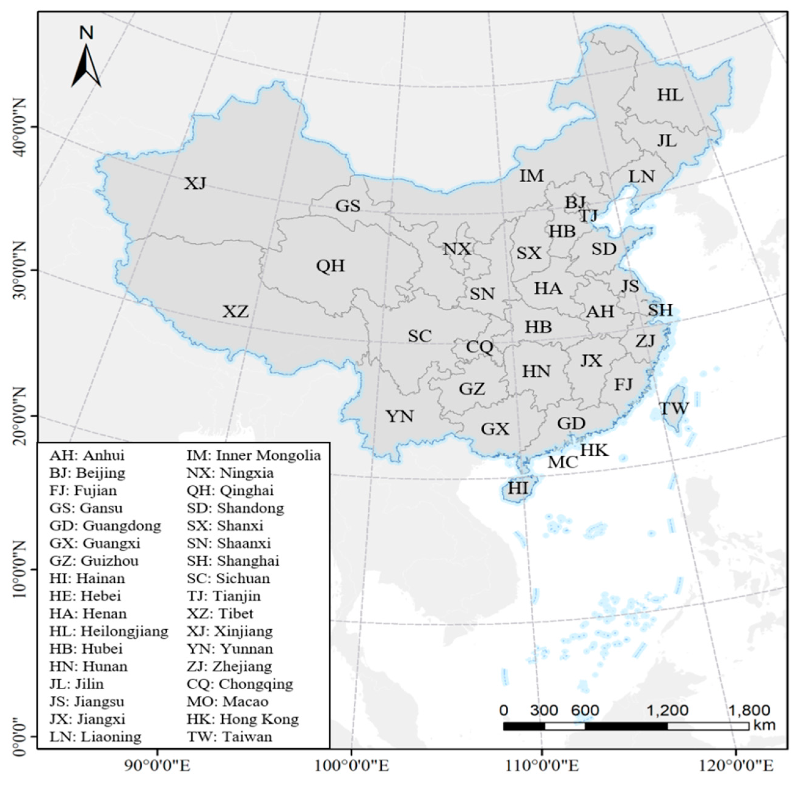
According to the parameters required in the Gompertz function, this study proceeds as follows. (1) We first estimated Gompertz models with different parameters using data from OECD countries, and then found appropriate models for the growth trend of vehicles for provinces in China. (2) Based on productivity convergence behaviors across economies, the labor productivity growth of provinces can be predicted. We predict the population growth rate and the employment rate of each province based on the characteristics of the population structure and employment participation rates. Finally, we get the potential growth rate of GDP by adding up the three rates and calculate GDP per capita for each province from 2020 to 2050. (3) We forecast future vehicle ownership for each province using the suitable Gompertz function. (4) We investigate the causes and factors that can affect the variation of vehicle ownership trends in different provinces. Figure 1 shows the map of China with the location of each province.
3.1. Gompertz Function
The Gompertz function has been widely used to study the relationship between vehicle ownership and economic factors [8,24,25,26,37]. Therefore, we estimate China’s provincial vehicle ownership from 2020 to 2050 using the Gompertz function as well. The Gompertz function is regularly expressed as:
where represents the number of vehicles per 1,000 people in region i in year t; represents the saturation level of vehicle ownership (vehicles per 1000 people) in region i; is GDP per capita in region i in year t; and and are negative parameters that determine the shape of the S-curves. The parameter α determines the demand of vehicle ownership at low or zero economic levels and the parameter β is a curvature parameter that controls the slope of the Gompertz function at high economic levels. The increase of α and β would lead to a steep S-shaped curve against the economic factors. Taking a log-linearization of Equation (1), we can get the following Equation:
Because historical data on China’s vehicle ownership is unavailable for a sufficiently long period, we estimate Equation (2) using data of the founding members of OECD countries, and try to find the suitable growth model of vehicle ownership for each province.
3.2. Selection of Suitable Gompertz Function
Most researchers estimate the same Gompertz function using all the historical data of several countries to predict China’s annual vehicle ownership [7]. However, the Gompertz functions may be different for each province because of variant economic characteristics across regions. So, it is necessary to investigate the most suitable vehicle ownership development model for each province and for each country. We try to estimate the Gompertz functions for each OECD country with enough samples, and then to select the optimum one for each province of China from these Gompertz functions. The specific steps are as follows. Firstly, we estimate the Gompertz function for each OECD country separately. Then we can obtain the estimated vehicles per 1000 people in province i in year t in country j by taking the actual GDP per capita of province i from 1991–2017 into Gompertz function of country j of OECD. Finally, we can find the optimal Gompertz function for each province by minimum the equation below:
where is the actual vehicle ownership of province i in year t.
3.3. Forecasting GDP per Capita
Bai and Zhang [16] note that the convergence law of transnational (regional) economic growth is mainly reflected in GDP per capita, rather than in total population change. For example, China’s investment and human capital are similar to those of Japan, Singapore, Korea and Taiwan at the same stage of development, but China’s employment rate in the total population is very different from the growth trends of these countries. Therefore, they use convergence trends in labor productivity in these countries to predict the growth rate of China’s labor productivity (LPG) and to predict the growth rate of China’s labor force (LFG) based on its own characteristics. We decompose the GDP growth rate of each province into LPG and LFG in the same way:
3.3.1. Forecasting Growth Rate of Labor Productivity
Compared with GDP per capita, GDP per labor reflects the performance of the economy from the perspective of production and can better reflect the actual situation of all labor resources in a certain period. The growth rates of laggards are usually higher than in developed economies according to the economic growth theory, and the convergence law of LPG can be expressed as the equation below [16,38]:
where is the growth rate of GDP per labor of province i in year t; is the growth rate of GDP per labor of the United States in year t-1; and and are parameters to be estimated. Parameter represents the growth rate of GDP per labor in the United States and parameter reflects the convergence rate of GDP per labor of the corresponding economy to the United States.
There are three comparable Asian economies (Japan, Korea, and Taiwan) whose economic convergence laws are similar to China according to the historical data. Firstly, according to the data of Penn World Table (PWT 9.0) [39], we can compare the GDP per capita of China with countries like Japan, Singapore, South Korea, and Taiwan, and it’s found that the GDP per capita of China in 2008 is similar with these countries in 1970s, and the investment and human capital is similar with these counties as well in the comparable periods. These facts bode well for the possibility that China, along with Japan, Singapore, South Korea and Taiwan, will experience similar growth paths at similar stages of development. Secondly, the four countries or districts, along with China, are all located in Asia, so they will share some common culture and economic growth pattern. Therefore, we choose them as the reference and use non-linear iteration to estimate the parameters and . To ensure the continuity and the comparability of data, the sample intervals of the three economies are Japan (1950-2014), Korea (1968-2014) and Taiwan (1965–2014), respectively. Data from the Penn World Table (PWT 9.0) [39] are only updated to 2014 and the GDP per capita of the United States and comparable Asian economies (Japan, South Korea and Taiwan) are calculated on the basis of output-side real GDP at chained PPPs in millions of 2011 US Dollars. After obtaining and , the annual growth rate of labor productivity of each province from 2020 to 2050 is estimated iteratively based on Equation (5) using the year 2014 as the starting point for prediction. Since the actual GDP published in Penn World Table (PWT9.0) [39] is based on 2011, we first convert the GDP index published by the National Bureau of Statistics into the GDP index based on 2011, and then get the actual per-labor GDP of each province in 2014 as the forecast point of this study. The iteration process is as follows. We assume that the annual growth rate of real GDP per labor in the United States between 2015 and 2050 is . Based on the actual GDP per labor of each province and the United States in 2014, it is easy to derive the growth rate of GDP per labor of each province in 2015. Then, we can get the values in 2016 based on the results of 2015, and so on.
3.3.2. Forecasting Growth Rate of Labor Force
Earlier studies have indicated that the growth rate of the labor force (LFG) does not converge like the growth of labor productivity does. Thus, it is more reasonable to predict the growth rate of the labor force of each province according to their individual characteristics. We divide the growth rate of labor force into two parts considering the theory and the availability of data:
where represents the growth rate of labor force of province i in year t, and is the growth rate of population of province i in year t, and is the growth rate of employment rate to the total population of province i in year t.
To derive the growth rate of population from 2020 to 2050, we must first predict the population in each year. Population prediction models include linear regression [40], autoregressive [41], Malthus [42,43,44], logistic [45], BP neural network [46,47], system dynamics [48,49], and Bayesian probabilistic projections [50,51,52]. Among these methods, the linear regression model is simple but more commonly used. As described in the linear regression model, at a certain period of population development, the population may show a linear growth trend in the short term. The regression model is as follows.
where t denotes the year; is the total population in year t, and and are the parameters to be estimated. Using historical population data from 1990 to 2017 (the data of some provinces such as Hubei, Chongqing, Sichuan and Guizhou are only from 2000 to 2017 because of data availability), the linear regression model is estimated to forecast the total population of each province from 2020 to 2050, and then we get the population growth rate. The growth rate of the employment rate of each province is estimated according to the following steps.
Firstly, we also use the linear model to predict the labor in each province, from which we can get the employment rate and its change in each province, combining the population results.
Secondly, we estimate the relationship between the proportion of employment and the proportion of population aged 15-64 at the nation level in a non-linear way as shown in Equation (8), referring to Bai and Zhang [34].
where represents China’s employed population in year t; represents China’s total population in year t; is the economically active population of China; and is China’s population aged 15–64.
Then we use the corresponding predictions of the proportion of population aged 15–64 in China published in World Population Prospects: 2017 to get the estimated value of China’s employment rate in 1978–2050, and then calculate its change rate. Additionally, in order to keep in line with the change of China’s employment population data, we adjust the growth rate of the employment rate of each province to make sure that the annually averaged growth rate of the employment rate of each province equals the nation-level value. Finally, Equation (6) is used to calculate the growth rate of the labor force in provinces from 2020 to 2050.
3.3.3. Forecasting GDP per Capita
Adding the growth rate of labor productivity and the growth rate of the labor force, we can derive the economic growth rate of provinces in 2018-2050. Then, based on the actual GDP of each province in 2017, it is easy to calculate the actual GDP of each province from 2018 to 2050, and the real GDP per capita of provinces from 2018 to 2050 are predicted given the population forecast.
3.4. Data
Our data is obtained from four sources. The first one is the World Road Statistics dataset (WRS), which is created by [53]. The WRS is the only universal source of strategic data on road networks, traffic and inland transport. It contains data on vehicle ownership in all OECD countries and in China from 1963 to 2011. There are two reasons and requirements when we choose the sample countries as benchmark. On the one hand, as the Gompertz function estimation needs long enough time series data, while Chinese vehicle ownership data is unavailable for a sufficiently long period, so we select the founding members of OECD countries that have enough samples. These countries include Australia, Austria, Belgium, Canada, Denmark, France, Germany, Ireland, Italy, Japan, the Netherlands, New Zealand, Norway, Spain, Sweden, Switzerland, United Kingdom and the United States. On the other hand, the pattern of vehicle ownership in these countries we choose can describe China’s vehicle stock growth [8,18].
The second one is Penn World Table (PWT 9.0) [39], which provides purchasing power parity and national income accounts converted to international prices for 182 countries during the years 1950-2014. Through PWT 9.0, we obtain real GDP data of China, the United States and three comparable Asian economies (Japan, Korea and Taiwan).
The third one is World Population Prospects: 2017 (WPP 2017) [54], which is the 25th round of population estimates and projections released by the United Nations Population Division. WPP 2017 forecasts the proportion of the total population aged 15–64 years from 2015 to 2050 for countries all over the world. Based on these data sets, according to Equation (8), we can calculate the proportion of employment to the total population of China.
Finally, we collect provincial GDP, the GDP index, the total population and the number of employed people from the China Statistical Yearbook [55], to forecast real GDP per capita of each province between 2020 and 2050. The data of vehicle ownership at the province level comes from the database of CIEC.
4. Results
4.1. Comparison of Vehicle Ownership Growth Models in Different Countries
The estimation results of the Gompertz model in each country are shown in Columns (1)–(18) of Table 1.
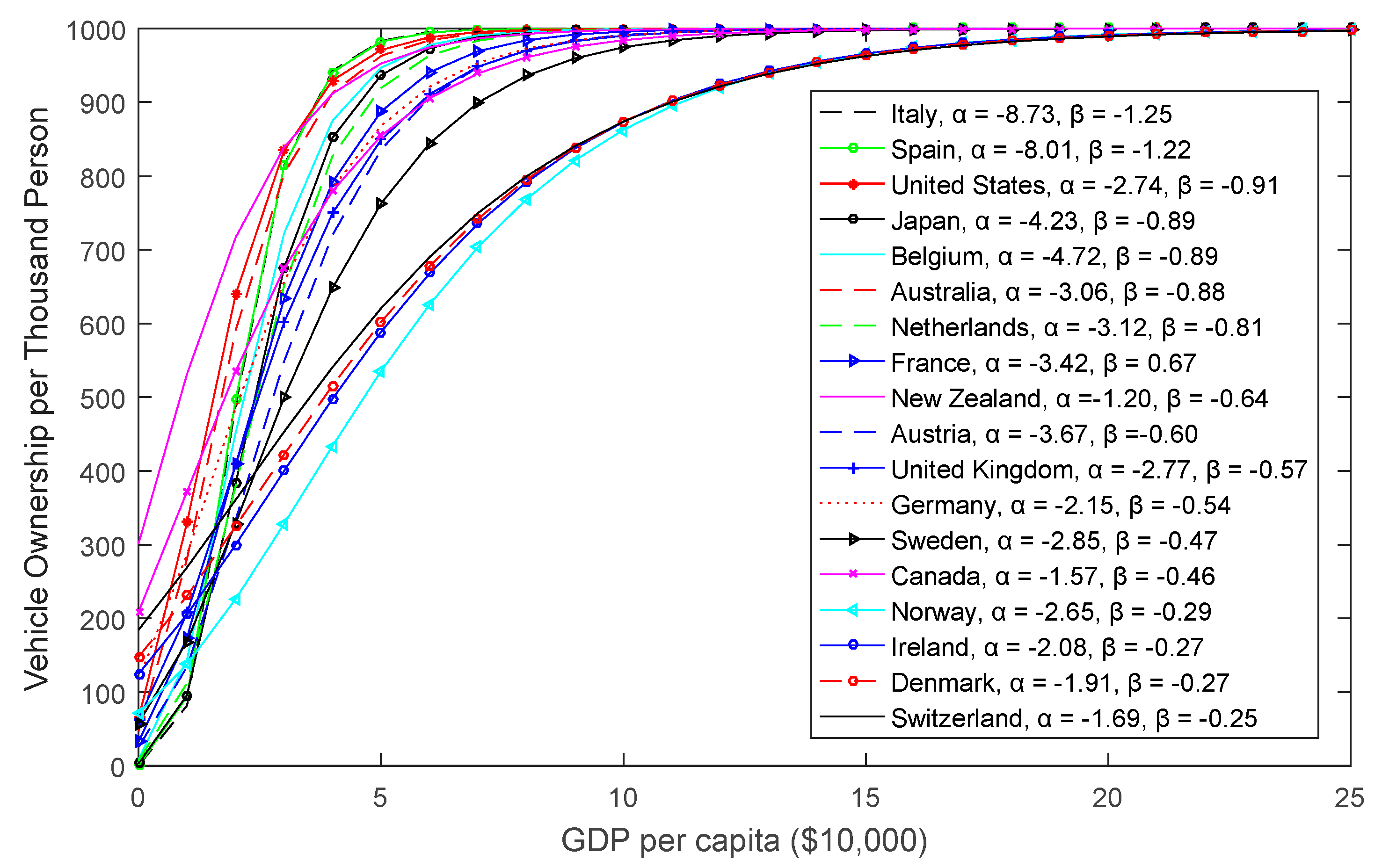
We can see that the coefficients of all columns are significant, and the adjusted R square is large enough, which mean the results of the regressions are valid. We can see that the countries with the highest growth include Italy, Spain and the United States, and the countries with lower growth rates are Sweden, Canada and Norway, which is consistent with the results of [8]. Figure 2 shows the S-curves of Gompertz functions of each country. The horizontal axis is GDP per capita ($10,000), and the vertical axis is the vehicle ownership per thousand people. The steeper the line is, the higher the vehicle growth rate will be.
4.2. Gompertz Mode Selection Applicable in China and Provinces
Table 2 shows the development models which are applicable to each province. The Belgium model, which belongs to the development model of European countries, is more suitable for China at the national level and is consistent with the conclusion of [8].
However, the development model of each province varies. For example, faster growth models, such as the Italian, Spanish, and Japanese models, are suitable to the vehicle ownership growth process of Inner Mongolia, Jiangsu, Fujian, Zhejiang, and Guangxi and Hunan, while the Netherlands model, which is a slightly faster growth model, is applicable to Hubei and Liaoning. Guangdong, Yunnan, Tibet, Guizhou and Shanxi are more like France and Austria, who have a slower growth rate of vehicle ownership. Vehicle ownership in Beijing, Shanghai and Tianjin grows slowest, which is similar to Norway.
4.3. Distribution of GDP Growth Rate and GDP per Capita
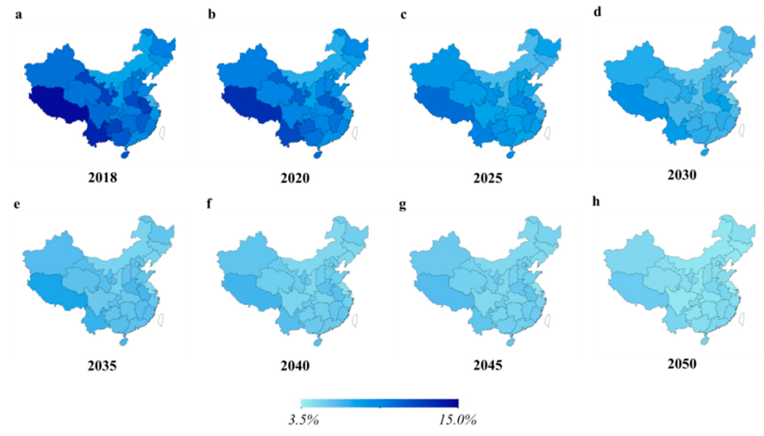
Figure 3 shows the growth rate of real GDP at each stage in each province. We only showed the results in years 2018, 2020, 2025, 2030, 2035, 2040, 2045, and 2050 for brevity, and we show the results in the same way in other tables and figures below. We can see that the average of economic growth rates is declining in each province. Since the development stage of each province is different, the GDP growth rates of each province is very different before 2030, but then converges to around 4.5%, which indicates that the continuous decline of potential economic growth in each province of China will become an inevitable trend in the future.
Figure 4 represents the results of the population forecast using the linear model and we can know that the distribution of population across province will not change greatly. We estimate the real GDP for each province for the next 30 years based on the estimated growth rate of GDP. GDP per capita can also be calculated combining with the population estimation. Table A1 shows the GDP per capita distribution of each province at different stages. In general, the real GDP per capita of each province is less than 20,000 US dollars in 2017. The highest level appears in Tianjin, which is about 19,000 US dollars, and the lowest level appears in Gansu, which is only about 4600 US dollars. GDP per capita of each province will increase every year, such that the GDP per capita in most provinces is about 50,000–90,000 US dollars by 2050.
4.4. Vehicle Ownership Forecast
Table 3 shows the forecasted vehicle ownership, based on GDP per capita in each province. The rate of vehicle ownership per thousand people in almost all provinces was no more than 200 in 2017, and it is more than 200 only in a few rich provinces, such as Guangdong, Beijing, Zhejiang and Jiangsu. This fact shows that the current vehicle ownership rate in China is currently still at a low level, which is consistent with other studies like [6,26]. However, in 2030, the number will be more than 300 vehicles in a majority of the provinces, and by 2040, the number will exceed 400 in all provinces, with some provinces reaching more than 600. By 2050, the number will exceed 500 in all of the provinces, reaching the highest in Zhejiang at 806. This indicates that the rate of vehicle ownership grows rapidly in each province of China and that some provinces will reach the saturation level, 807, according to [26].
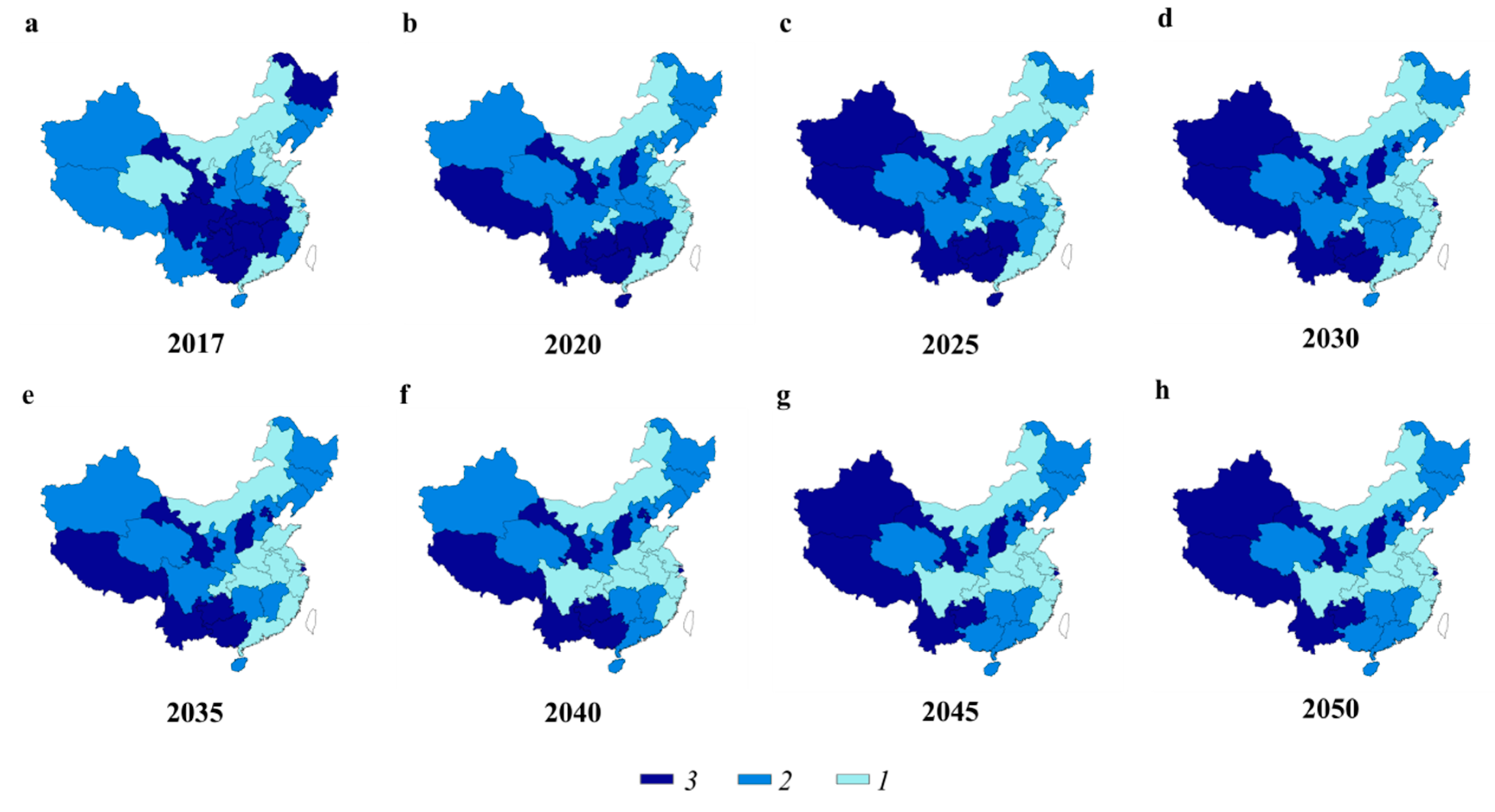
In order to show the trend of vehicle ownership of each province in a more intuitive way, we divide the provinces into high (labeled by 1), medium (labeled by 2) and low (labeled by 3) groups according to their ranks. Figure 5 shows the group number of vehicle ownership in each province in different years. It can be seen that the ranking changes greatly over this period. The ranking of some provinces with higher vehicle ownership in 2017, such as Guangdong, Tianjin, Ningxia, Qinghai, Hebei and Beijing, will decline in the following years, especially Beijing and Tianjin. In the middle-level group, the ranking of provinces such as Shanghai, Xinjiang, Shanxi, Tibet and Yunnan will also decline in the next 30 years, and they will fall into the low-level group.
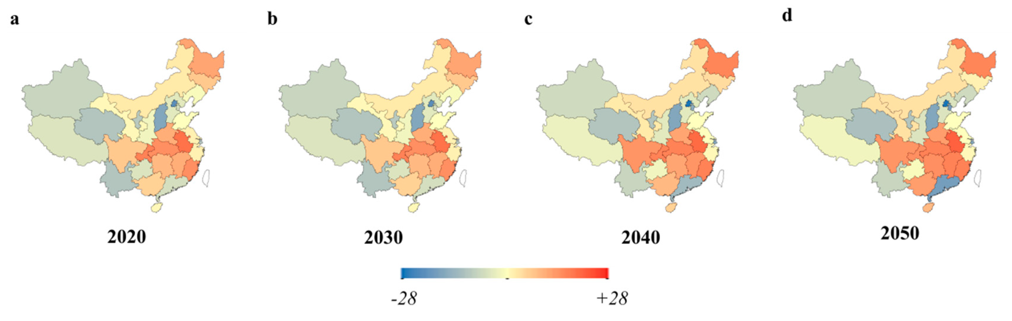
Secondly, the ranking of Fujian and Henan, which are in the middle level group in 2017, will increase in the following years, while the rankings of Chongqing, Hubei, Anhui and Sichuan, which are currently in the low-ranking group, will increase to the higher level group. Heilongjiang, Jiangxi, Hunan and Guangxi, which are also in low level group in 2017, will have middle-level vehicle ownership. Finally, the vehicle ownership of Inner Mongolia, Zhejiang, Jiangsu, Shandong, Jilin, Liaoning, Shaanxi, Hainan, Gansu and Guizhou will remain at a medium level. Figure 6 shows the specific changes in the rankings of vehicle ownership in each province relative to the 2017.
5. Factors That Affect the Trend of Vehicle Ownership in Each Province
The ranking of vehicle ownership of most provinces in the future will change and the speed and extent of growth varies across provinces. There are several features in the growth process: (1) Higher-ranking provinces will tend to decline in the future, while the lower ones will tend to increase in the future; (2) the current first-tier provinces, such as Beijing, Shanghai, Tianjin, and Guangdong will fall into the low-level vehicle ownership group in 2050. We will analyze several causes that lead to these results.
5.1. Differences in the Growth Model of Vehicle Ownership
The vehicle growth model has a great impact on the growth speed and the ranking of vehicle ownership in each province. Just as Table 2 shows, the model with rapid growth rate can partially explain why some provinces can keep their high rankings in the next 30 years, such as Inner Mongolia, Zhejiang, Jiangsu and Shandong, which is shown in Table 2.
The average-speed growth model leads to the unchanged ranking of some provinces with middle-level vehicle ownership now, such as Jilin, Liaoning, Shaanxi, Hainan, Gansu and Guangxi. The slow growth rate of the vehicle ownership model can partly explain why some provinces have declining rankings. For example, the development model with low-growth rate, which is only 0.289, is applicable to Beijing, Shanghai and Tianjin. The growth-rate parameter of Guangdong’s model is 0.671, which is still below the national average. Similarly, the slower growth rate in Tibet, Yunnan, and Shanxi provinces also led to the decline in their rankings. The faster vehicle growth model is more likely to lead to increasing ranking, such as Fujian Province, who will rise to the high vehicle ownership group from the middle group now.
5.2. Differences in GDP per Capita and Its Growth Rate
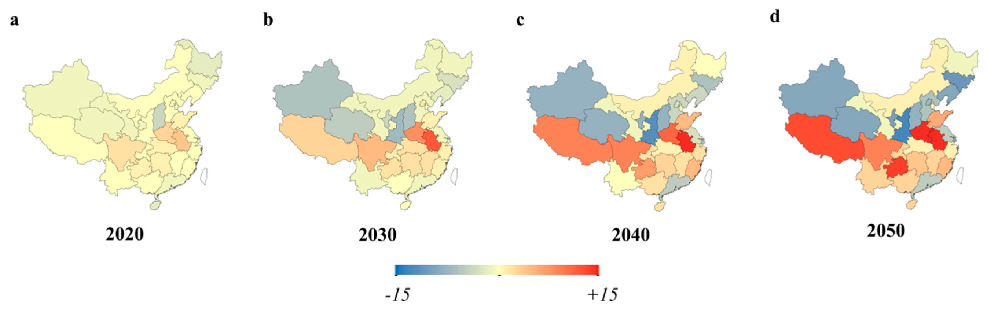
Another important factor in the Gompertz model is GDP per capita. We also group each province into high (labeled by 1), medium (labeled by 2) and low (labeled by 3) groups according to their ranking of GDP per capita. Figure 7 shows the group number of each province. It can be seen that the ranking of GDP per capita in each province is basically consistent with the ranking of vehicle ownership, especially before 2025. This result shows that GDP per capita also has a great impact on the vehicle ownership of each province. The ranking of GDP per capita of each province changes after 2025. Some provinces in the middle group now will jump to the high-level group, such as Chongqing and Henan, or fall into the low-level group, such as Xizang, Shanxi, Guangdong and Liaoning. The ranking of some provinces in the low-level group now will increase, such as Sichuan and Hunan, which explains the rise in their vehicle ownership rankings. Figure 8 shows the detailed changes of ranking of GDP per capita of each province.
Table 4 shows the growth rate of GDP per capital of each province in different years. The province order is sorted by the 2018 value. It can be seen that there exist stepwise changes from the lower left corner to the upper right corner, which is consistent with the distribution trend of GDP per capita, and current GDP per capita is negatively correlated with its growth rate. For example, the growth rate of GDP per capita is only about 5% in rich province like Beijing and Shanghai, and it will gradually decline to around 3% in the next 30 years. The value in Tianjin and Jiangsu will decline to around 3% from around 6%, and Henan, Hunan, Guangxi and Guizhou will have the highest values, which is about 5% in 2050. The growth rate of GDP per capita will decline from the range of 7–13% to the range of 3–5% in 2050 in other provinces. The difference in the growth rates of GDP per capita across provinces ultimately led to differences in GDP per capita, which in turn will affect vehicle ownership.
Vehicle ownership is more likely to increase rapidly in provinces with a higher growth rate of GDP per capita under the same development model. For example, in Henan, Anhui, Sichuan, Jiangxi and Hunan provinces, the GDP growth rate per capita is more than 10% in 2018, so it will converge slowly in the next 30 years, which can lead to rapid growth in GDP per capita, and thus rapid growth in vehicle ownership. This phenomenon also exists in the three provinces of Chongqing, Hubei and Heilongjiang, whose growth rate of GDP per capita is 9%. The growth rate of GDP per capita is around 8% in the provinces like Shaanxi, Jilin and Shandong, whose vehicle growth rate is also on the average level, so that their ranking of vehicle ownership will not change much in the next 30 years. The ranking is likely to decline in provinces with a middle or low-level growth rate of GDP per capita and low growth rate of vehicle growth model, such as Guangdong, Xinjiang, Ningxia, Qinghai, Shanxi, Hebei, Hubei, especially Beijing, Shanghai and Tianjin. While the ranking may increase in provinces with low GDP per capita growth rates but rapid growth model of vehicle, such as Jiangsu, Inner Mongolia and Zhejiang. The growth rate of GDP per capita is 7% in these provinces, but the suitable vehicle growth pattern is the Italy and Spain model, which has a high growth rate, so their vehicle ownership is always high ranked.
5.3. The Growth Rate of GDP per Labor and Employment Proportion
The growth rate of GDP per capita can be decomposed into the growth rate of GDP per labor and the growth rate of the employment rate. Therefore, we compare the two factors across provinces.
The estimated result of parameters in Equation (5) is μ = 2.427%, θ = 0.673. We use the year 2014 as the starting point to obtain the growth rate of GDP per labor of each province by iteration from 2018 to 2050. The results are shown in Table A2. The order of the provinces is sorted by the 2018 value. It can be seen that from the lower left corner to the upper right corner, the growth rate of GDP per labor is similar to the growth rate of GDP per capita, which also presents step changes, indicating that the growth rate of GDP per labor is a major factor determining the growth rate of GDP per capita. The growth rate of GDP per capita presents more tidy and rigorous step changes, which is consistent with the economic convergence theory. However, due to the different development stages, the average GDP growth rate is different in each province, and the growth rate of GDP per labor is more dispersed than the growth rate of GDP per capita in 2018.
A high growth rate of GDP per capita leads to rapid increases in vehicle ownership. The provinces with average growth rate of GDP per labor probably keep their ranking unchanged or even drop when their growth rate in the Gompertz function is low, such as in Guangdong, Xinjiang, Ningxia, Qinghai, Shanxi, Hebei and Hubei. Similarly, the low growth rate of GDP per labor usually leads to the low level of vehicle ownership, such as in Beijing, Shanghai and Tianjin. The exception appears when the growth rate in Gompertz function is high, for instance, Jiangsu and Inner Mongolia and Zhejiang provinces, whose suitable models are Italy and Spain, and will remain in the top in the ranking of vehicle ownership.
Table A3 shows the growth rate of the employment rate in each province, which reflects the difference between the growth rate of GDP per capita and GDP per labor. We can see two phenomena in this table. (1) The value of the growth rate is almost negative, and the negative value becomes even smaller in each province, which means the employment proportion decreases in the future. This is consistent with national level results predicted by [16]. There are two reasons for this: First, the demographic dividends, which contributed a lot to economic growth in the past decades in China, are disappearing because of the aging population. The population and labor structure still maters but they begin to have a negative effect on the economic growth rate. Second, with the development of artificial intelligence and automation, many jobs are replaced by machines, so that a reduction in employment opportunities will lead to a decline in the employment rate. (2) The provinces with a lower GDP growth rate per labor, such as Shanghai, Jiangsu, Beijing and Tianjin, have lower growth rates of the employment rate, and this leads to a lower growth rate of GDP per capita and the decline of vehicle ownership rankings. The growth rate of the employment rate is higher, even positive in the provinces in the lower development stages, such as Tibet and Heilongjiang. This is because, although there are more employment opportunities in the more developed provinces, the artificial intelligence and automation penetration rate is high, so more employment is replaced by machines. More labor must migrate back to the less-developed provinces, which leads to the high growth rate of employment in these areas. Some western provinces, such as Gansu and Qinghai, cannot attract people due to their poor industrial structure. Thus, the employment in these regions will drop a lot as well in the future.
6. Regional Analysis
In order to analyze the connections and differences between provinces, we focus on the characteristics of the trend of vehicle ownership in the five regions. The Yangtze River Delta includes Shanghai, Jiangsu, Zhejiang and Anhui; the Pearl River Delta includes Guangdong, Fujian, and Hainan; the Bohai Bay region includes Beijing, Tianjin, Hebei, and Shandong; the Guanzhong-Bashu includes Shaanxi, Chongqing, and Sichuan; and the western region includes Guangxi, Guizhou, Yunnan, Tibet, Gansu, Qinghai, Ningxia and Xinjiang. Although the five regions don’t include all of China’s provinces, they are representative enough to allow us to analyze the characteristics of regions that are united by several provinces. And there are several development policies placed on these regions which can help us understand the connections in these regions. Table 5 shows the vehicle ownership forecast of each region. It can be seen that vehicle ownership trends are similar in each region. Vehicle ownership is almost around 700 by the end of 2050, which means the development among each region is similar. This character also exists in the growth rate of GDP per labor and employment proportion, which is shown in Table 6 and Table 7. Except for the western region and the Guanzhong-Bashu region, whose growth rate of GDP per labor is a little higher, regions all start to converge from around 7% to 4% by 2050. Table 7 shows the growth rate of employment proportion in the five major regions, and we can see the largest drop of employment appears in Guanzhong-Bashu district, and the decreasing of employment degree is similar in other regions.
There are several reasons for the phenomenon. First, there are interactions between provinces in each region. Although there are differences in each province within each region, they may develop with complementarity and mutual cooperation, so there will be no large weaknesses smoothing out the regional growth rate. Second, the government will always coordinate the balanced development of large areas in its long-term development strategies. A lot of development strategies to promote balanced regional development have been announced. In recent years, the government has successively implemented coordinated development strategies in of Beijing-Tianjin-Hebei, the Yangtze River Delta, the Guanzhong Tianshui Economic Zone and the Chengdu-Chongqing Economic Zone. These development strategies are mainly achieved through industrial support policies and supporting funds, which directly affect the employment of the labor force and internal and external labor mobility in the supported regions, thus affecting the proportion of employment in the region. This will also affect the industrial layout in the region and the infiltration and application of technology in the industry, which will indirectly affect the labor productivity in the region, thus affecting the growth rate of GDP per labor in the region.
Therefore, China’s coordinating regional development strategy will not only promote the balance development of regions and achieve effective allocation of production factors within the region, but also can achieve effective allocation of elements between regions by the movement of labor and technology diffusion, and then affect the growth rate of GDP per labor and the change of employment proportion. The two effects together will affect the regional growth rate of GDP per capita, so that the vehicle development of each region will finally show a convergence trend.
7. Robustness Check
7.1. Malthus Population Growth Model
We do several checks to make our results robust. First, beside the linear growth model of population, Malthus [56] argues that the natural growth rate of population is a constant. Assuming that the population in the initial period is and the population growth rate is , the population of year is approximately:
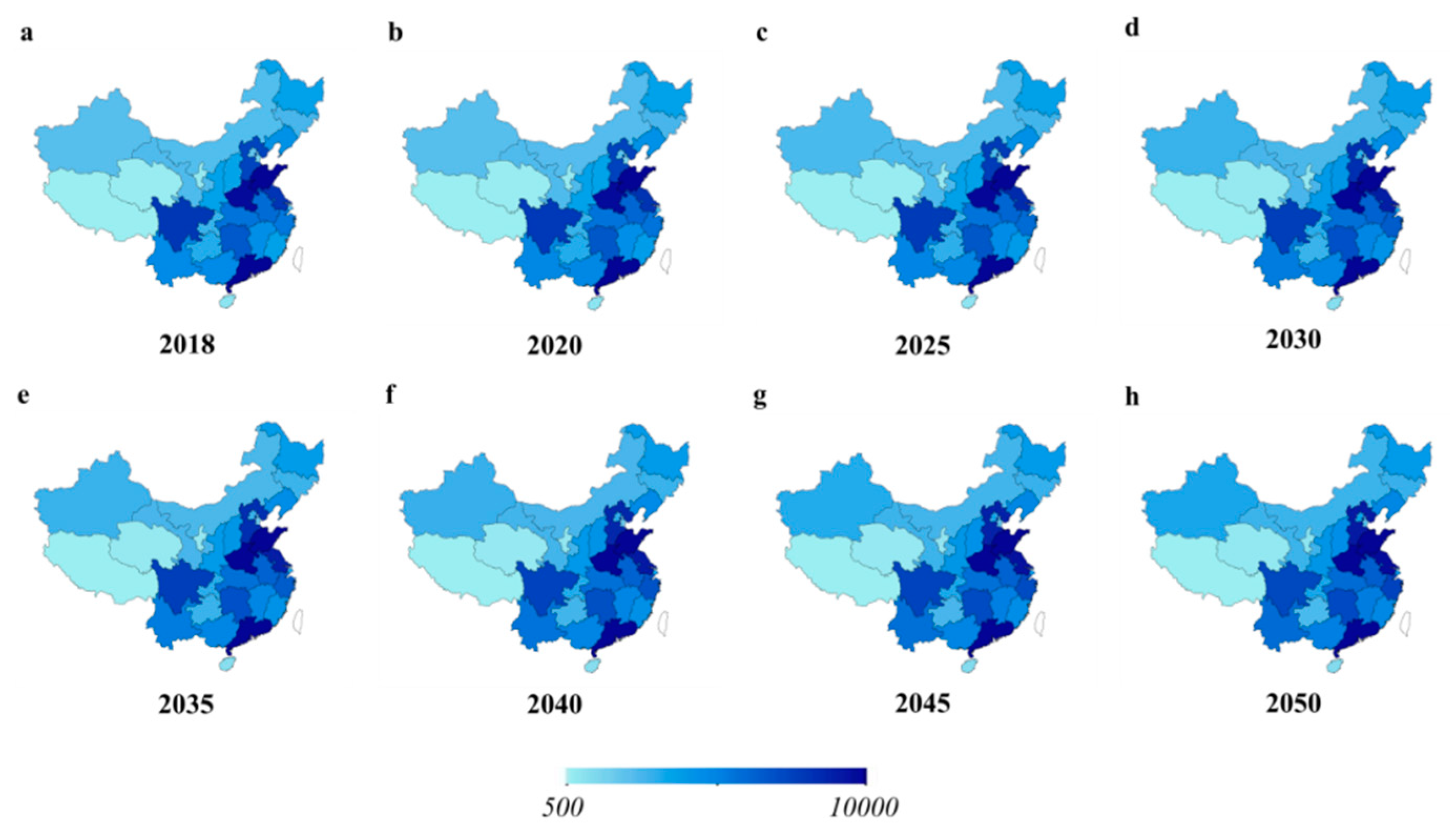
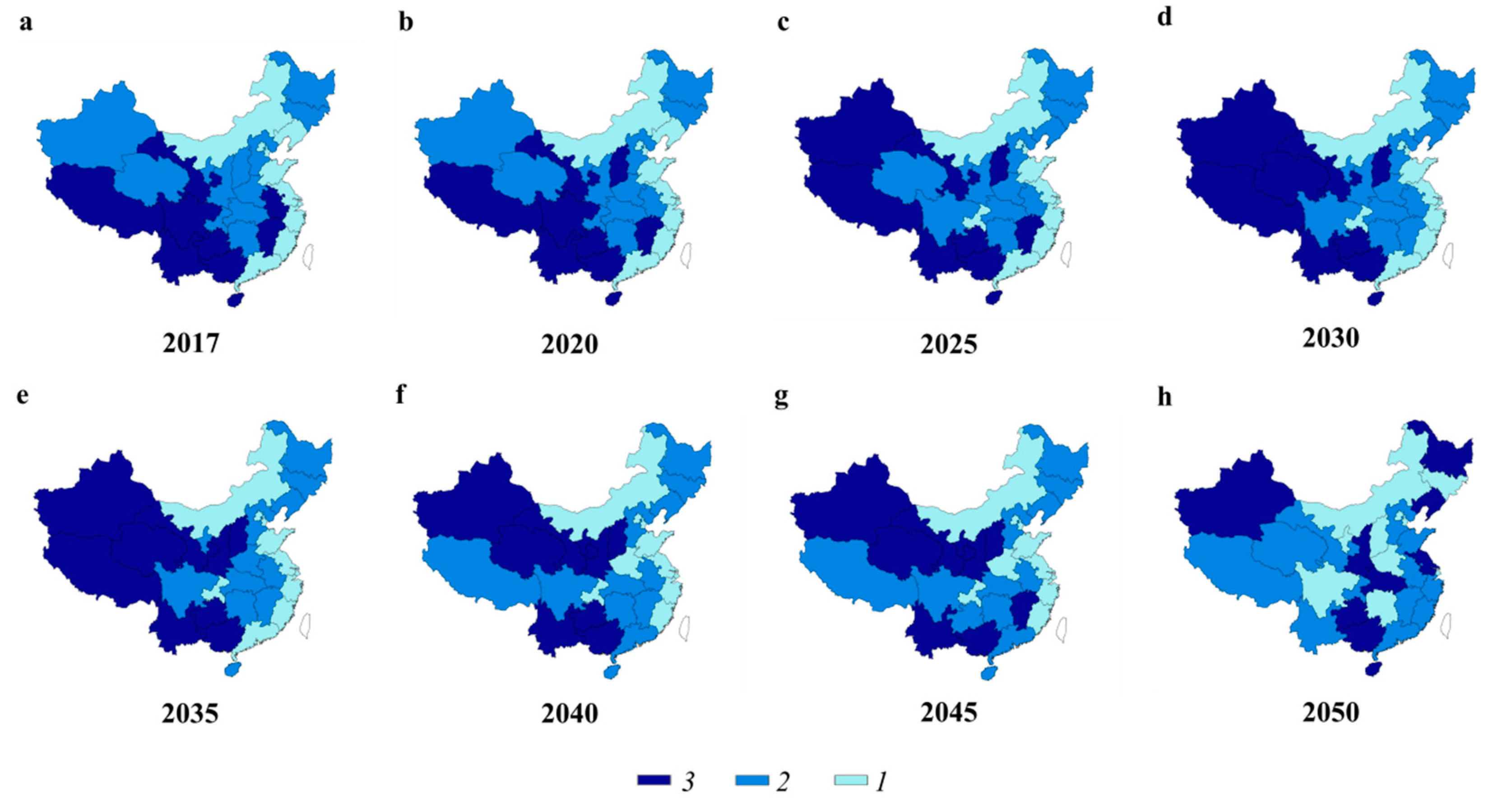
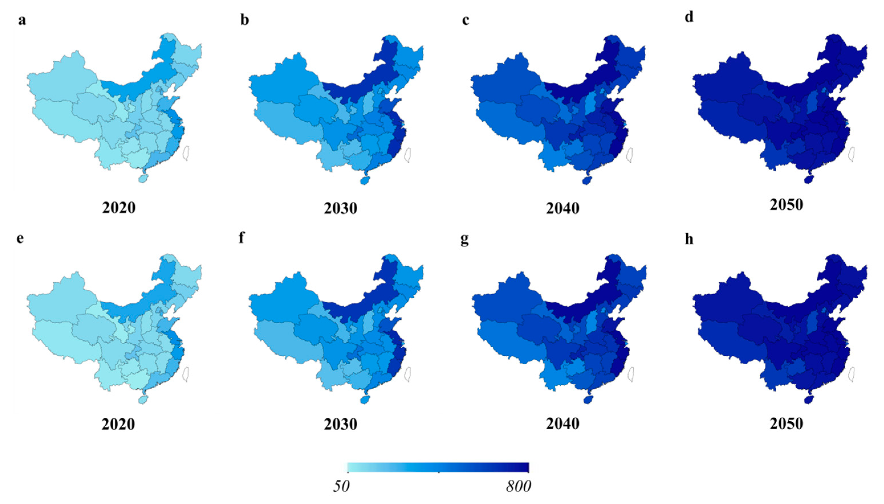
We use the Malthus model to make population forecast as well. From this we get the GDP per capita, combing the real GDP results we estimated before and estimating the vehicle ownership in each province using the Gompertz model. The estimated results are shown in Picture e-h, Figure 9, and we can see that the results are similar with the ones using the linear population model, which are shown in Picture a-d, Figure 9. Compared with the results of Table 3, we can see the trend of vehicle ownership more clearly. The vehicle ownership distribution is unbalanced in the beginning, and the eastern provinces have most vehicles, especially the coastal provinces, however, the western provinces will catch up in the future. We also see the lighter blue color in Beijing and Tianjin, which is consistent with the results above. The only small difference between the results of the two methods is that, the blue color is a little lighter in Picture h than Picture d, which means the increasing speed of western provinces, is a little slower if we use Malthus population growth model in the process of GDP per capita estimation. Maybe this is because the population growth is faster in Malthus model and then the GDP per capita is smaller, and finally leads to lower vehicle ownership.
7.2. Gompertz Model with Different Saturation Levels
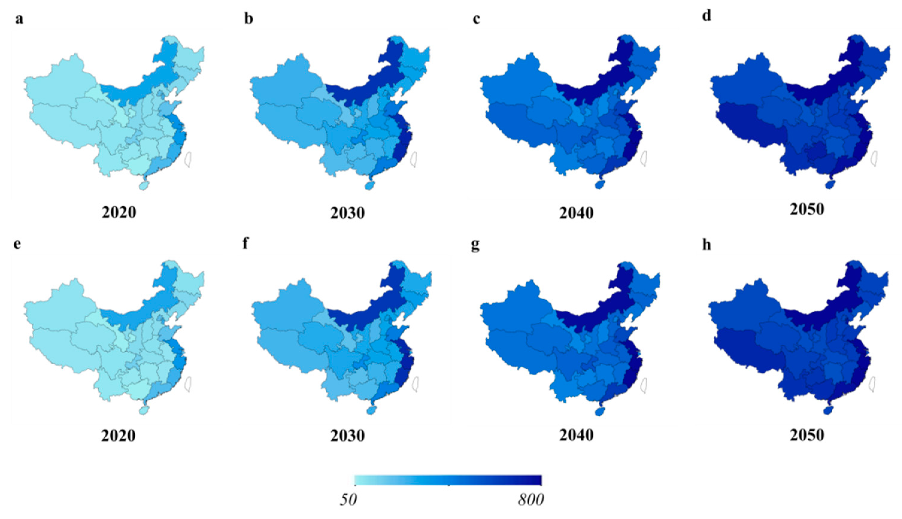
Second, we make the provincial vehicle ownership forecast in each province using the Gompertz model with different saturation levels. We set the saturation level for each province equal to the saturation value of the country whose Gompertz model is suitable to this province and the saturation level of each country comes from [26]. The forecast results with the linear and the Malthus population models are shown in Figure 10. The results are still similar with Figure 9. We can see that the vehicle ownership will increase in all of the provinces and the distribution is becomes more balanced in year 2050 than year 2020 because the increasing speed is larger in western provinces than that in the eastern provinces. The difference between Figure 10 and Figure 9 is that, the vehicle ownership in the provinces of middle area is smaller in Figure 10 than Figure 9 because the blue color is lighter in pictures of Figure 10. This is because that the saturation levels are small in their applicable Gompertz models, which means the saturation levels will affect the estimation results but not that much, so we can still get the similar results.
7.3. Absolute Value Criterion to Choose Optimal Vehicle Growth Model for Each Province
We try to use another criterion to choose optimal vehicle ownership growth model for each province. Just as Equation (3), we estimate the Gompertz function for each OECD country separately. Then we can obtain the estimated vehicles per 1000 people in province i in year t in country j by taking the actual GDP per capita of province i from 1991–2017 into Gompertz function of country j of OECD. Finally we can find the optimal Gompertz function for each province with the equation below:
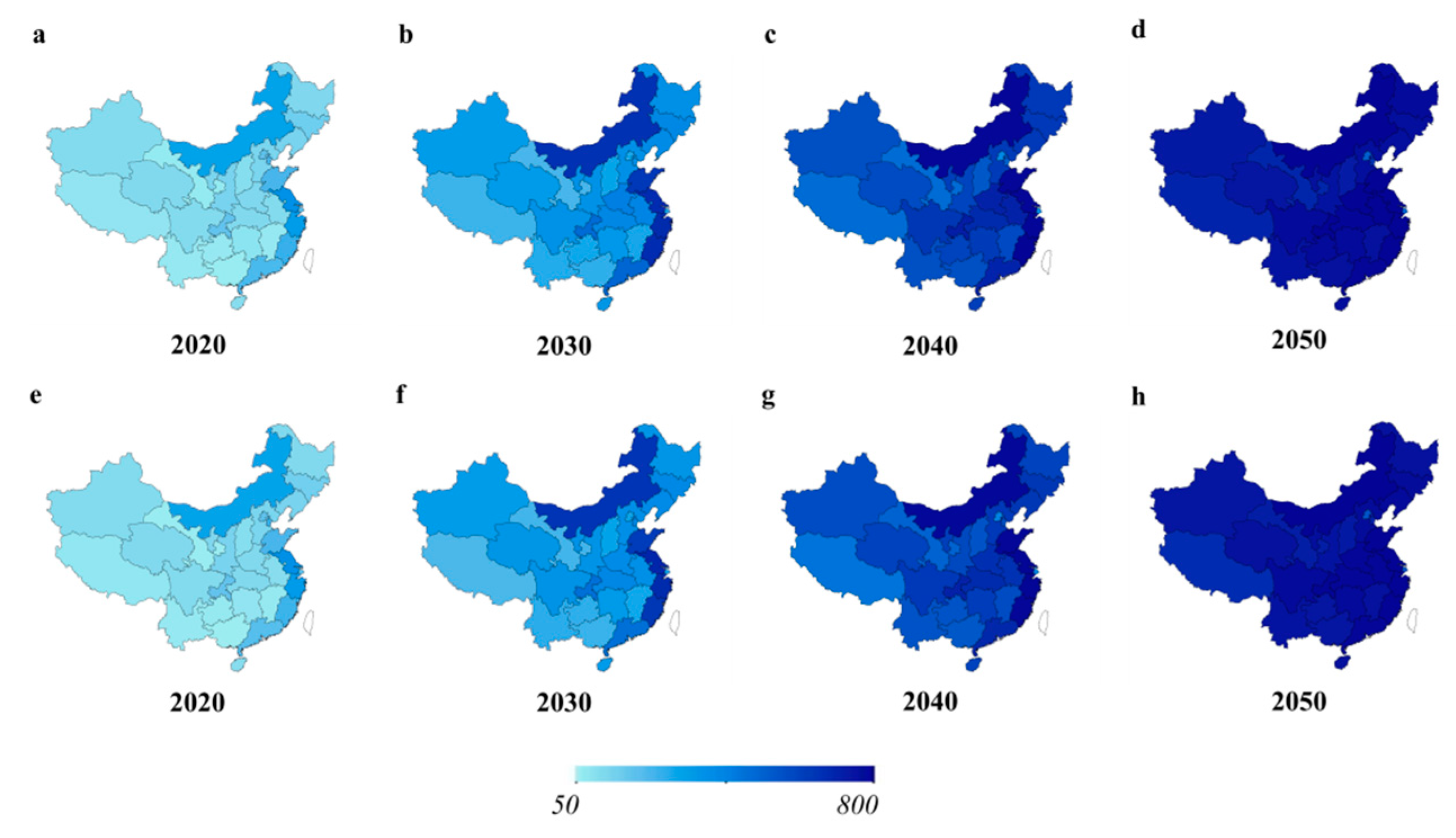
where is the actual vehicle ownership of province i in year t, which is just the same as before in Section 3.2. Figure 11 presents the estimated vehicle ownership results in each province with common saturation levels (we show the estimated results with different saturation levels in each province in Figure A1, which is similar with this result). Picture a–d shows the results of using linear population growth from 2020 to 2050, respectively, while Picture e–f shows the results of using Malthus population growth model. We can see that the results are still similar with our results before, which means the results is robust no matter we use what criterion to choose optimal vehicle ownership growth model for each province. We still can get the result that the vehicle ownership in the western province will increase in the future, even large than some middle provinces.
8. Conclusions
The growth of vehicle production is not only the result of economic development, but also an important driving force for economic development and for industrial development. However, the increase of vehicle ownership has also triggered environmental problems, the severity of which varies in different provinces. Only by accurately predicting vehicle ownership, building a high-quality supply of vehicles, and following up sales with support services and industrial development planning can we make full use of the advantages of the vehicle industry. It is of great significance to build supporting infrastructure and other services based on accurate forecasts of vehicle ownership in various provinces because of the variance of economic development, the carrying capacity of resources, and different degrees of transport planning in each province.
We used the Gompertz model to predict China’s provincial vehicle ownership from 2018 to 2050. Considering the impact of the population structure, we summed up the growth rate of GDP per labor, the population and the employment rate to get the growth rate of GDP and then the GDP per capita of each province. We found that the vehicle ownership rate in each province will grow rapidly in the next 30 years; however, the change in the ranking of vehicle ownership among provinces varies. Then, we analyzed the causes that affect the change of ranking. On the one hand, the suitable growth pattern, which is reflected by the coefficient in the Gompertz model, has an important effect on vehicle ownership. On the other hand, the GDP per capita is another key factor that affects vehicle ownership. The stage of economic development and government policy are related to the growth rate of GDP per labor and employment rate, which then affect GDP per capita.
Therefore, we propose the following suggestions: first, the rapid growth of vehicle ownership, especially the rapid growth of traditional internal combustion engine vehicles, brings the increasing consumption of oil. Therefore, the government needs to accelerate the growth rate of new energy vehicles to replace the consumption of oil of traditional internal combustion engine vehicles. Second, from our result, the vehicle ownership will be balanced all over the country because the increasing need of undeveloped province in the future, so it is necessary for the government to make capacity planning and give some policy for the vehicle industry to ensure and induce the balanced expansion in the western area to meet the increasing demand of vehicle. Third, although the pollution problems are paid high attention by the government and society in eastern and developed provinces, the government and vehicle companies should do some preparation in some western province, because the vehicle ownership will grow fast in 30 years according to our forecast, and limit pollution within a reasonable level to better promote economic and green development.
There are some limitations in our research. First, it is impossible to divide the car ownership of traditional internal combustion engine vehicles and electric vehicles because of data availability. For example, the state has different purchase restrictions on these two types of cars in Beijing. Second, the benchmark countries we use are only OECD countries because of data availability as well. Our results will be more precise if we have more sample data of the benchmark countries or state level vehicle ownership data of U.S. or other region level data of comparable countries to China. Finally, some policies that can tense the decreasing of employment, for instants, universal two-child policy and delay the retirement policy are not included in the GDP per capital estimation process.
In the follow-up research, we will try to investigate several topics as below: firstly, since the degree of development of shared bikes or cars varies in different provinces, we will consider the influence of the penetration rate of shared travel market and the substitution and combined travel mode of shared car and private car travel on the prediction of car ownership in different provinces. Secondly, we will consider more policies that can affect the results in the estimation process, e.g. tensing the purchase restrictions, universal two-child policy and delay the retirement policy. Thirdly, we will use state level of U.S. or other region level data of comparable countries to China to estimate Gompertz function. Finally, we will do some research about the impact of vehicle ownership on other economic variables, for example, transportation, environment pollution, employment and so on, in order to prepare for the growth of vehicle ownership.
Author Contributions
All authors were involved in preparing the manuscript. T.W. and L.M. contributed to the design of the research framework and conceptualization and developed methodology. L.M., M.W. and X.T. conducted empirical analysis and wrote the manuscript. G.Z. conducted the visualization part including the tables and figures. Q.D. contributed to the GDP forecasting and policy implications.
Funding
This research was funded by the National Natural Science Foundation of China, grant number [71703022, 71804181 and 71774095] and the National Center for Mathematics and Interdisciplinary Sciences, CAS.
Conflicts of Interest
The authors declare no conflict of interest.
Appendix A

Table A1.
GDP Per capita of each province at different stages (10,000 USD).
| Province | 2017 | 2020 | 2025 | 2030 | 2035 | 2040 | 2045 | 2050 |
|---|---|---|---|---|---|---|---|---|
| Tianjin | 1.87 | 2.61 | 3.39 | 4.27 | 5.23 | 6.28 | 7.52 | 8.88 |
| Shanghai | 1.78 | 2.13 | 2.65 | 3.24 | 3.87 | 4.55 | 5.35 | 6.23 |
| Beijing | 1.68 | 2.11 | 2.65 | 3.26 | 3.91 | 4.62 | 5.46 | 6.38 |
| Jiangsu | 1.49 | 1.92 | 2.49 | 3.14 | 3.83 | 4.59 | 5.49 | 6.47 |
| Zhejiang | 1.33 | 1.79 | 2.43 | 3.16 | 3.98 | 4.89 | 5.98 | 7.18 |
| Inner Mongolia | 1.32 | 1.75 | 2.34 | 3.04 | 3.81 | 4.68 | 5.73 | 6.9 |
| Fujian | 1.15 | 1.6 | 2.29 | 3.12 | 4.07 | 5.16 | 6.49 | 8 |
| Shandong | 1.1 | 1.53 | 2.17 | 2.93 | 3.79 | 4.77 | 5.97 | 7.31 |
| Guangdong | 1.11 | 1.46 | 1.98 | 2.58 | 3.23 | 3.96 | 4.83 | 5.78 |
| Liaoning | 0.99 | 1.31 | 1.78 | 2.32 | 2.91 | 3.58 | 4.38 | 5.27 |
| Chongqing | 0.92 | 1.31 | 1.87 | 2.55 | 3.33 | 4.23 | 5.31 | 6.54 |
| Hubei | 0.84 | 1.21 | 1.75 | 2.4 | 3.14 | 3.99 | 5.01 | 6.16 |
| Jilin | 0.89 | 1.18 | 1.63 | 2.15 | 2.73 | 3.38 | 4.16 | 5.02 |
| Shaanxi | 0.83 | 1.11 | 1.52 | 2 | 2.53 | 3.13 | 3.85 | 4.65 |
| Ningxia | 0.76 | 1.05 | 1.5 | 2.02 | 2.6 | 3.25 | 4.02 | 4.89 |
| Hebei | 0.74 | 1.05 | 1.51 | 2.05 | 2.66 | 3.34 | 4.16 | 5.08 |
| Hunan | 0.72 | 1.05 | 1.54 | 2.12 | 2.78 | 3.54 | 4.44 | 5.46 |
| Henan | 0.69 | 1.02 | 1.58 | 2.28 | 3.12 | 4.1 | 5.32 | 6.74 |
| Heilongjiang | 0.74 | 1.02 | 1.48 | 2.03 | 2.67 | 3.4 | 4.29 | 5.31 |
| Qinghai | 0.71 | 0.98 | 1.4 | 1.89 | 2.43 | 3.04 | 3.75 | 4.55 |
| Xinjiang | 0.69 | 0.97 | 1.38 | 1.85 | 2.38 | 2.98 | 3.68 | 4.47 |
| Anhui | 0.63 | 0.97 | 1.52 | 2.23 | 3.06 | 4.06 | 5.29 | 6.73 |
| Sichuan | 0.63 | 0.95 | 1.43 | 2 | 2.67 | 3.43 | 4.36 | 5.43 |
| Jiangxi | 0.65 | 0.94 | 1.4 | 1.94 | 2.57 | 3.28 | 4.13 | 5.09 |
| Hainan | 0.65 | 0.94 | 1.39 | 1.94 | 2.57 | 3.28 | 4.14 | 5.1 |
| Shanxi | 0.65 | 0.91 | 1.3 | 1.75 | 2.26 | 2.83 | 3.52 | 4.27 |
| Guangxi | 0.59 | 0.87 | 1.31 | 1.84 | 2.44 | 3.14 | 3.99 | 4.95 |
| Tibet | 0.5 | 0.79 | 1.27 | 1.87 | 2.56 | 3.37 | 4.35 | 5.46 |
| Yunnan | 0.49 | 0.74 | 1.16 | 1.68 | 2.28 | 2.97 | 3.79 | 4.72 |
| Guizhou | 0.45 | 0.72 | 1.16 | 1.71 | 2.37 | 3.17 | 4.17 | 5.38 |
| Gansu | 0.46 | 0.69 | 1.06 | 1.5 | 1.99 | 2.54 | 3.2 | 3.93 |
Note: the larger value is represented by darker blue, and the smaller value is represented by lighter blue.
Table A2.
Growth rate of GDP per labor in each province (%).
| Province | 2018 | 2020 | 2025 | 2030 | 2035 | 2040 | 2045 | 2050 |
|---|---|---|---|---|---|---|---|---|
| Beijing | 5.69 | 5.46 | 4.98 | 4.61 | 4.31 | 4.07 | 3.87 | 3.70 |
| Shanghai | 5.71 | 5.48 | 5.00 | 4.62 | 4.32 | 4.07 | 3.87 | 3.70 |
| Tianjin | 6.56 | 6.23 | 5.56 | 5.06 | 4.67 | 4.36 | 4.11 | 3.90 |
| Jiangsu | 6.63 | 6.29 | 5.60 | 5.09 | 4.69 | 4.38 | 4.12 | 3.91 |
| Inner Mongolia | 6.89 | 6.51 | 5.77 | 5.22 | 4.79 | 4.46 | 4.19 | 3.97 |
| Zhejiang | 7.50 | 7.04 | 6.14 | 5.50 | 5.01 | 4.63 | 4.33 | 4.08 |
| Liaoning | 7.51 | 7.05 | 6.15 | 5.50 | 5.01 | 4.63 | 4.33 | 4.08 |
| Guangdong | 7.52 | 7.06 | 6.16 | 5.51 | 5.02 | 4.64 | 4.33 | 4.08 |
| Shaanxi | 7.74 | 7.24 | 6.29 | 5.60 | 5.09 | 4.69 | 4.38 | 4.12 |
| Jilin | 8.17 | 7.60 | 6.53 | 5.78 | 5.23 | 4.80 | 4.46 | 4.19 |
| Shandong | 8.40 | 7.80 | 6.67 | 5.88 | 5.30 | 4.86 | 4.51 | 4.23 |
| Fujian | 8.42 | 7.82 | 6.68 | 5.89 | 5.31 | 4.86 | 4.51 | 4.23 |
| Chongqing | 8.75 | 8.09 | 6.86 | 6.02 | 5.40 | 4.94 | 4.57 | 4.28 |
| Xinjiang | 8.99 | 8.28 | 6.99 | 6.11 | 5.47 | 4.99 | 4.61 | 4.31 |
| Ningxia | 9.10 | 8.38 | 7.05 | 6.15 | 5.50 | 5.01 | 4.63 | 4.33 |
| Heilongjiang | 9.23 | 8.48 | 7.12 | 6.20 | 5.54 | 5.04 | 4.66 | 4.35 |
| Shanxi | 9.23 | 8.48 | 7.12 | 6.20 | 5.54 | 5.04 | 4.66 | 4.35 |
| Heibei | 9.38 | 8.61 | 7.20 | 6.26 | 5.58 | 5.07 | 4.68 | 4.37 |
| Hubei | 9.53 | 8.73 | 7.28 | 6.31 | 5.62 | 5.11 | 4.71 | 4.39 |
| Qinghai | 9.54 | 8.74 | 7.29 | 6.31 | 5.62 | 5.11 | 4.71 | 4.39 |
| Hunan | 10.03 | 9.13 | 7.54 | 6.49 | 5.75 | 5.20 | 4.78 | 4.45 |
| Jiangxi | 10.45 | 9.49 | 7.76 | 6.64 | 5.86 | 5.29 | 4.85 | 4.50 |
| Hainan | 10.46 | 9.48 | 7.75 | 6.64 | 5.86 | 5.28 | 4.84 | 4.50 |
| Sichuan | 10.64 | 9.63 | 7.85 | 6.70 | 5.90 | 5.32 | 4.87 | 4.52 |
| Guangxi | 10.91 | 9.84 | 7.98 | 6.79 | 5.97 | 5.37 | 4.91 | 4.55 |
| Henan | 11.11 | 9.99 | 8.07 | 6.85 | 6.01 | 5.40 | 4.93 | 4.57 |
| Anhui | 11.82 | 10.55 | 8.40 | 7.07 | 6.16 | 5.51 | 5.02 | 4.64 |
| Gansu | 12.24 | 10.87 | 8.59 | 7.19 | 6.25 | 5.57 | 5.07 | 4.68 |
| Guizhou | 12.63 | 11.16 | 8.76 | 7.30 | 6.32 | 5.63 | 5.11 | 4.71 |
| Yunnan | 12.81 | 11.30 | 8.83 | 7.35 | 6.36 | 5.65 | 5.13 | 4.73 |
| Tibet | 13.09 | 11.52 | 8.96 | 7.43 | 6.41 | 5.69 | 5.16 | 4.75 |
Note: the larger value is represented by darker blue, and the smaller value is represented by lighter blue.
Table A3.
Growth rate of employment rate of each province (%).
| Province | 2018 | 2020 | 2025 | 2030 | 2035 | 2040 | 2045 | 2050 |
|---|---|---|---|---|---|---|---|---|
| Shanghai | −0.67 | −0.64 | −0.56 | −0.67 | −0.85 | −0.75 | −0.56 | −0.85 |
| Jiangsu | −0.56 | −0.55 | −0.49 | −0.62 | −0.81 | −0.73 | −0.54 | −0.84 |
| Gansu | −0.51 | −0.50 | −0.45 | −0.57 | −0.78 | −0.69 | −0.51 | −0.81 |
| Qinghai | −0.47 | −0.46 | −0.41 | −0.54 | −0.74 | −0.66 | −0.48 | −0.77 |
| Beijing | −0.45 | −0.44 | −0.40 | −0.53 | −0.73 | −0.65 | −0.47 | −0.77 |
| Tianjin | −0.42 | −0.41 | −0.37 | −0.50 | −0.71 | −0.64 | −0.46 | −0.76 |
| Jilin | −0.31 | −0.30 | −0.26 | −0.39 | −0.60 | −0.53 | −0.35 | −0.65 |
| Shanxi | −0.27 | −0.27 | −0.23 | −0.37 | −0.59 | −0.52 | −0.34 | −0.65 |
| Liaoning | −0.25 | −0.24 | −0.20 | −0.34 | −0.55 | −0.48 | −0.30 | −0.61 |
| Ningxia | −0.24 | −0.24 | −0.21 | −0.36 | −0.58 | −0.51 | −0.34 | −0.65 |
| Hebei | −0.22 | −0.21 | −0.18 | −0.32 | −0.54 | −0.47 | −0.30 | −0.60 |
| Guangdong | −0.21 | −0.21 | −0.20 | −0.35 | −0.58 | −0.52 | −0.35 | −0.66 |
| Hunan | −0.20 | −0.20 | −0.16 | −0.29 | −0.50 | −0.43 | −0.25 | −0.55 |
| Xinjiang | −0.20 | −0.20 | −0.19 | −0.34 | −0.57 | −0.50 | −0.34 | −0.65 |
| Shaanxi | −0.20 | −0.19 | −0.15 | −0.29 | −0.50 | −0.43 | −0.26 | −0.56 |
| Zhejiang | −0.18 | −0.18 | −0.16 | −0.31 | −0.53 | −0.47 | −0.30 | −0.61 |
| Jiangxi | −0.15 | −0.14 | −0.11 | −0.26 | −0.47 | −0.41 | −0.24 | −0.55 |
| Sichuan | −0.14 | −0.13 | −0.07 | −0.19 | −0.39 | −0.30 | −0.11 | −0.39 |
| Hubei | −0.14 | −0.13 | −0.09 | −0.22 | −0.43 | −0.35 | −0.17 | −0.47 |
| Yunnan | −0.12 | −0.12 | −0.10 | −0.25 | −0.47 | −0.41 | −0.24 | −0.55 |
| Guangxi | −0.11 | −0.10 | −0.07 | −0.20 | −0.42 | −0.35 | −0.17 | −0.48 |
| Hainan | −0.04 | −0.04 | −0.03 | −0.20 | −0.43 | −0.37 | −0.21 | −0.53 |
| Inner Mongolia | −0.04 | −0.03 | 0.00 | −0.15 | −0.37 | −0.31 | −0.14 | −0.45 |
| Heilongjiang | 0.06 | 0.06 | 0.10 | −0.04 | −0.25 | −0.18 | −0.01 | −0.31 |
| Shandong | 0.10 | 0.10 | 0.12 | −0.03 | −0.26 | −0.21 | −0.05 | −0.36 |
| Guizhou | 0.11 | 0.13 | 0.22 | 0.14 | −0.01 | 0.12 | 0.37 | 0.14 |
| Chongqing | 0.15 | 0.15 | 0.16 | 0.01 | −0.22 | −0.16 | 0.00 | −0.32 |
| Tibet | 0.24 | 0.22 | 0.19 | 0.00 | −0.25 | −0.22 | −0.08 | −0.41 |
| Anhui | 0.35 | 0.35 | 0.39 | 0.25 | 0.03 | 0.10 | 0.27 | −0.04 |
| Fujian | 0.35 | 0.34 | 0.33 | 0.15 | −0.10 | −0.07 | 0.08 | −0.25 |
| Henan | 0.37 | 0.37 | 0.40 | 0.25 | 0.03 | 0.09 | 0.26 | −0.05 |
Note: the larger value is represented by darker blue, and the smaller value is represented by lighter blue.
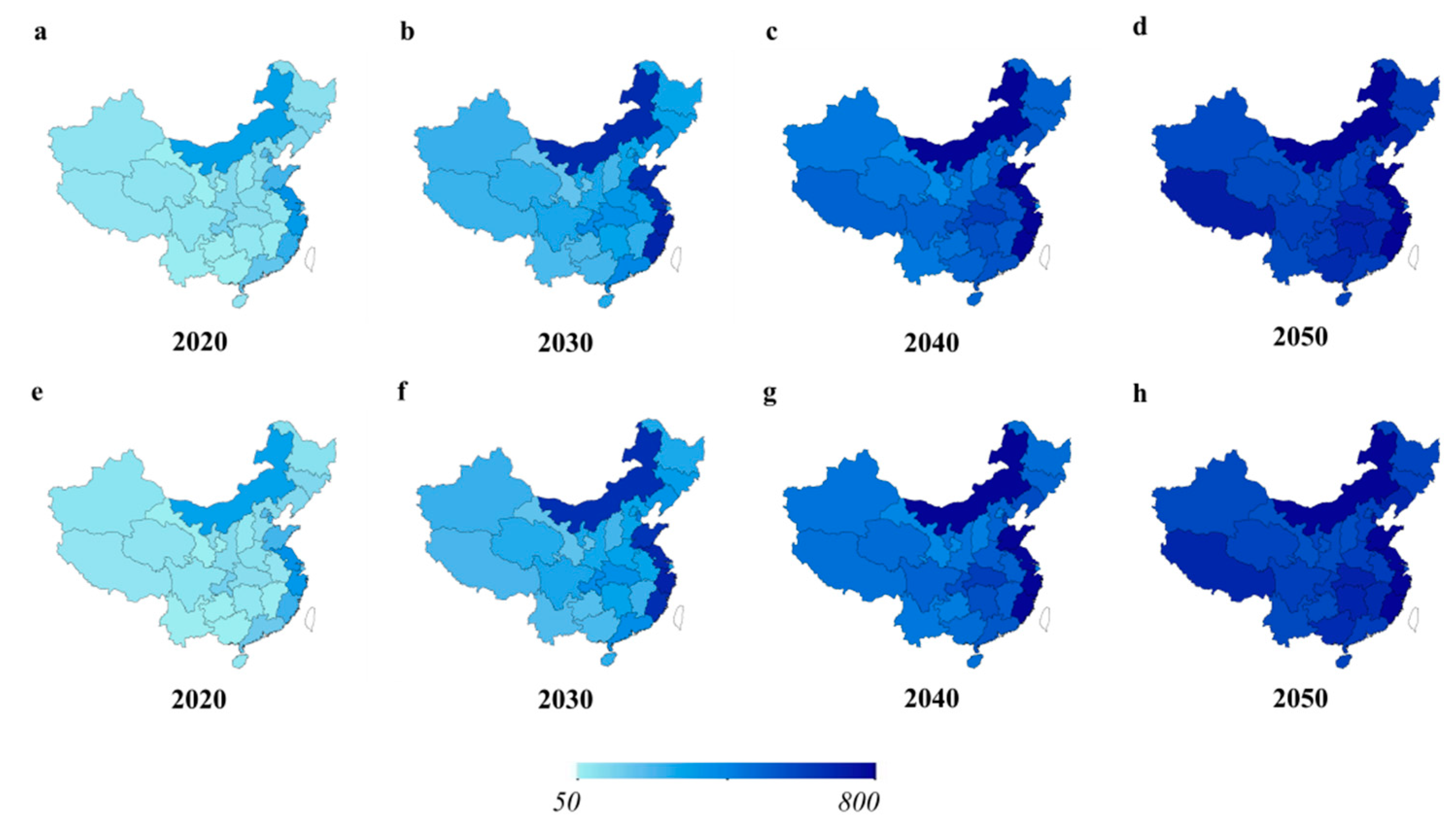
Figure A1.
Vehicle ownership forecast of Linear and Malthus population model with common saturation levels.
Figure A1.
Vehicle ownership forecast of Linear and Malthus population model with common saturation levels.

References
- Huo, H.; Zhang, Q.; He, K.; Yao, Z.; Wang, X.; Zheng, B.; David, G.; Wang, Q.; Ding, Y. Modeling vehicle emissions in different types of Chinese cities: Importance of vehicle fleet and local features. Environ. Pollut. 2011, 159, 2954–2960. [Google Scholar] [CrossRef] [PubMed]
- Yang, Z.; Jia, P.; Liu, W.; Yin, H. Car ownership and urban development in Chinese cities: A panel data analysis. J. Transp. Geogr. 2017, 58, 127–134. [Google Scholar] [CrossRef]
- Burrow, M.; Evdorides, H.; Wehbi, M.; Savva, M. The benefits of sustainable road management: A case study. Transport 2013, 166, 222–232. [Google Scholar] [CrossRef]
- Burrow, M.P.N.; Evdorides, H.; Ghataora, G.S.; Petts, R.; Snaith, M.S. The evidence for rural road technology in low-income countries. Transport 2016, 169, 366–377. [Google Scholar] [CrossRef] [Green Version]
- Qian, L.; Soopramanien, D. Using diffusion models to forecast market size in emerging markets with applications to the Chinese car market. J. Bus. Res. 2014, 67, 1226–1232. [Google Scholar] [CrossRef]
- Richter, A.; Burrows, J.P.; Nub, H.; Granier, C.; Niemeier, U. Increase in tropospheric nitrogen dioxide over China observed from space. Nature 2005, 437, 129–132. [Google Scholar] [CrossRef] [PubMed]
- Wu, Y.; Wang, R.; Zhou, Y.; Lin, B.; Fu, L.; He, K.; Hao, J. On-road vehicle emission control in Beijing: Past, present, and future. Environ. Sci. Technol. 2011, 45, 147–153. [Google Scholar] [CrossRef] [PubMed]
- Wu, T.; Zhang, M.; Ou, X. Analysis of future vehicle energy demand in China based on a Gompertz function method and computable general equilibrium model. Energies 2014, 7, 7454–7482. [Google Scholar] [CrossRef]
- Zeng, Y.; Tan, X.; Gu, B.; Xu, B. Greenhouse gas emissions of motor vehicles in Chinese cities and the implication for China’s mitigation targets. Appl. Energy 2016, 184, 1016–1025. [Google Scholar] [CrossRef]
- Zhang, X.; Rao, R.; Xie, J.; Liang, Y. The current dilemma and future path of China’s electric vehicles. Sustainability 2014, 6, 1567–1593. [Google Scholar] [CrossRef]
- Yu, J.; Yang, P.; Zhang, K.; Wang, F.; Miao, L. Evaluating the effect of policies and the development of charging infrastructure on electric vehicle diffusion in China. Sustainability 2018, 10, 3394. [Google Scholar] [CrossRef]
- Ma, L.; Zhai, Y.; Wu, T. Operating charging infrastructure in China to achieve sustainable transportation: The choice between company-owned and franchised structures. Sustainability 2019, 11, 1549. [Google Scholar] [CrossRef]
- Das, D.; Sharfuddin, A.; Datta, S. Personal vehicles in Delhi: Petrol demand and carbon emission. Int. J. Sustain. Transp. 2009, 3, 122–137. [Google Scholar] [CrossRef]
- Waraich, R.A.; Galus, M.D.; Dobler, C.; Balmer, M.; Andersson, G.; Axhausen, K.W. Plug-in hybrid electric vehicles and smart grids: Investigations based on a microsimulation. Transp. Res. Part. C Emerg. Technol. 2013, 28, 74–86. [Google Scholar] [CrossRef] [Green Version]
- Chen, X.; Zhang, H. Evaluation of effects of car ownership policies in Chinese megacities: Beijing and Shanghai. Transp. Res. Rec. J. Transp. Res. Board 2012, 2317, 32–39. [Google Scholar] [CrossRef]
- Bai, C.; Zhang, Q. China’s growth potential to 2050: A supply-side forecast based on cross-country productivity convergence and its featured labor force. China Journal of Economics 2017, 4, 1–27. [Google Scholar]
- Li, Y.; Tian, Y.; Li, C.; Zhou, X. A prediction of vehicle possession in Hunan province based on principal component and BP neural network. Adv. Mater. Res. 2011, 403–408, 1337–1341. [Google Scholar] [CrossRef]
- Wu, T.; Zhao, H.; Ou, X. Vehicle ownership analysis based on GDP per capita in China: 1963–2050. Sustainability 2014, 6, 4877–4899. [Google Scholar] [CrossRef]
- Jong, G.D.; Fox, J.; Daly, A.; Pieters, M.; Smit, R. Comparison of car ownership models. Transp. Rev. 2004, 24, 379–408. [Google Scholar] [CrossRef]
- Azadeh, A.; Neshat, N.; Rafiee, K.; Zohrevand, A.M. An adaptive neural network-fuzzy linear regression approach for improved car ownership estimation and forecasting in complex and uncertain environments: The case of Iran. Transp. Plan. Technol. 2012, 35, 221–240. [Google Scholar] [CrossRef]
- Mogridge, M.J.H. The prediction of car ownership. J. Transp. Econ. Policy 1967, 1, 52–74. [Google Scholar]
- Pendyala, R.M.; Kostyniuk, L.P.; Goulias, K.G. A repeated cross-sectional evaluation of car ownership. Transportation 1995, 22, 165–184. [Google Scholar] [CrossRef]
- Potoglou, D.; Kanaroglou, P.S. Modelling car ownership in urban areas: A case study of Hamilton, Canada. J. Transp. Geogr. 2008, 16, 42–54. [Google Scholar] [CrossRef]
- He, K.; Huo, H.; Zhang, Q.; He, D.; An, F.; Wang, M.; Walsh, M.P. Oil consumption and CO2 emissions in China’s road transport: Current status, future trends, and policy implications. Energy Policy 2005, 33, 1499–1507. [Google Scholar] [CrossRef]
- Huo, H.; Wang, M. Modeling future vehicle sales and stock in China. Energy Policy 2012, 43, 17–29. [Google Scholar] [CrossRef]
- Dargay, J.; Sommer, G.M. Vehicle ownership and income growth, worldwide: 1960-2030. Energy J. 2007, 28, 143–170. [Google Scholar] [CrossRef]
- Dargay, J.; Gately, D. Vehicle ownership to 2015: Implications for energy use and emissions. Energy Policy 1997, 25, 1121–1127. [Google Scholar] [CrossRef]
- Dargay, J.; Gately, D. Income’s effect on car and vehicle ownership, worldwide: 1960–2015. Transp. Res. Part. A: Policy Pract. 1999, 33, 101–138. [Google Scholar] [CrossRef]
- Huo, H.; Wang, M.; Johnson, L.; He, D. Projection of Chinese motor vehicle growth, oil demand, and CO2 emissions through 2050. Transp. Res. Rec. J. Transp. Res. Board 2007, 2038, 69–77. [Google Scholar] [CrossRef]
- Carlucci, F.; Cirà, A.; Lanza, G. Hybrid electric vehicles: Some theoretical considerations on consumption behaviour. Sustainability 2018, 10, 1302. [Google Scholar] [CrossRef]
- Lu, H.; Ma, H.; Sun, Z.; Wang, J. Analysis and prediction on vehicle ownership based on an improved stochastic Gompertz diffusion process. J. Adv. Transp. 2017, 2017, 1–8. [Google Scholar] [CrossRef]
- Lian, L.; Tian, W.; Xu, H.; Zheng, M. Modeling and forecasting passenger car ownership based on symbolic regression. Sustainability 2018, 10, 2275. [Google Scholar] [CrossRef]
- Brandt, L.; Ma, D.; Rawski, T. From divergence to convergence: Reevaluating the history behind China’s economic boom. J. Econ. Lit. 2013, 52, 45–123. [Google Scholar] [CrossRef]
- Eichengreen, B.; Park, D.; Shin, K. When fast-growing economies slow down: International evidence and implications for China. Asian Econ. Pap. 2012, 11, 42–87. [Google Scholar] [CrossRef]
- Zhang, Y.; Lou, F. Analysis and forecast on the potential of China’s economic growth. Quant. Tech. Econ. Res. 2009, 26, 137–145. [Google Scholar]
- Cai, F.; Lu, Y. Population change and resulting slowdown in potential GDP growth in China. China World Econ. 2013, 21, 1–14. [Google Scholar] [CrossRef]
- Zhao, H. The medium and long term forecast of China’s vehicle stock per 1000 person based on the Gompertz model. J. Ind. Technol. Econ. 2012, 31, 7–23. [Google Scholar]
- Lucas, R.E., Jr. Trade and the diffusion of the industrial revolution. Am. Econ. J. Macroecon. 2009, 1, 1–25. [Google Scholar] [CrossRef]
- Feenstra, R.C.; Inklaar, R.; Timmer, M.P. The next generation of the Penn World Table. Am. Econ. Rev. 2015, 105, 3150–3182. [Google Scholar] [CrossRef]
- Tang, J.; Zhao, X. A comparative study on the population prediction models in land use planning. China Land Sci. 2005, 2, 14–20. [Google Scholar]
- Fan, Y.; Wang, G.; Sun, L. Research on Chinese population aging speed based on the ARMA model. Adv. Mater. Res. 2014, 926–930, 1168–1171. [Google Scholar] [CrossRef]
- Seidl, I.; Tisdell, C.A. Carrying capacity reconsidered: From Malthus’ population theory to cultural carrying capacity. Ecol. Econ. 1999, 31, 395–408. [Google Scholar] [CrossRef]
- Pingle, M. Introducing dynamic analysis using Malthus’s principle of population. J. Econ. Educ. 2003, 34, 3–20. [Google Scholar] [CrossRef]
- Abu, J.; Okwori, J.; Ajegi, S.O.; Ochinyabo, S. An empirical investigation of Malthusian population theory in Nigeria. J. Emerg. Trends Econ. Manag. Sci. 2015, 6, 367–375. [Google Scholar]
- Chen, Y. Carrying capacity estimation of Logistic model in population and resources prediction by nonlinear autoregression. J. Nat. Resour. 2009, 24, 1105–1114. [Google Scholar]
- Li, G.; Wu, T.; Xu, S. Prediction model of population gross based on grey artificial neural network and its application. Comput. Eng. Appl. 2009, 45, 215–218. [Google Scholar]
- Jia, N.; Hu, H.; Bai, Y. Population prediction based on BP artificial neural network. J. Shandong Univ. Technol. 2011, 10, 3297–3301. [Google Scholar]
- Andrew, M.; Meen, G. Population structure and location choice: A study of London and South East England. Pap. Reg. Sci. 2010, 85, 401–419. [Google Scholar] [CrossRef]
- Wu, P.; Wu, Q.; Dou, Y. Simulating population development under new fertility policy in China based on system dynamics model. Qual. Quant. 2017, 51, 2171–2189. [Google Scholar] [CrossRef]
- Raftery, A.E.; Alkema, L.; Gerland, P. Bayesian population projections for the United Nations. Stat. Sci. A Rev. J. Inst. Math. Stat. 2012, 29, 58. [Google Scholar] [CrossRef] [PubMed]
- Raftery, A.E.; Chunn, J.L.; Gerland, P. Bayesian probabilistic projections of life expectancy for all countries. Demography 2013, 50, 777–801. [Google Scholar] [CrossRef] [PubMed]
- Fosdick, B.; Raftery, A.E. Regional probabilistic fertility forecasting by modeling between-country correlations. Demogr. Res. 2014, 30, 1011–1034. [Google Scholar] [CrossRef] [PubMed] [Green Version]
- International Road Federation. IRF World Road Statistics 2013; International Road Federation Press: Vernier Geneva, Switzerland, 2013. [Google Scholar]
- United Nations. World Population Prospects: The 2017 Revision; United Nations: New York, NY, USA, 2017; Available online: https://www.un.org/development/desa/publications/world-population-prospects-the-2017-revision.html (accessed on 13 April 2019).
- National Statistics Bureau. China Statistical Yearbook; National Statistics Bureau: Beijing, China, 2018. Available online: http://www.stats.gov.cn/tjsj/ndsj/ (accessed on 16 April 2019).
- Malthus, T.R. An Essay on the Principle of Population; Cambridge University Press: Cambridge, UK, 1798. [Google Scholar]
Figure 1.
Map of China with province names and locations.

Figure 2.
Simulation of vehicle ownership growth in each country.

Figure 3.
GDP growth rate for each province from 2020 to 2050.

Figure 4.
Population distribution for each province from 2020 to 2050 (10,000 people).

Figure 5.
The ranking group of vehicle ownership of each province.

Figure 6.
The specific ranking change of vehicle ownership of each province.

Figure 7.
The ranking group of GDP per capita of each province.

Figure 8.
The specific ranking changes of GDP per capita of each province.

Figure 9.
Vehicle ownership forecast of Linear and Malthus population model.

Figure 10.
Vehicle ownership forecast of Linear and Malthus population model with different saturation levels.
Figure 10.
Vehicle ownership forecast of Linear and Malthus population model with different saturation levels.

Figure 11.
Vehicle ownership forecast of Linear and Malthus population model with common saturation levels.
Figure 11.
Vehicle ownership forecast of Linear and Malthus population model with common saturation levels.

Table 1.
Estimation results of national Gompertz models.
| (1) | (2) | (3) | (4) | (5) | (6) | |
| Australia | Austria | Belgium | Canada | Denmark | France | |
| EF | −0.878*** | −0.604*** | −0.891*** | −0.460*** | −0.265*** | −0.671*** |
| (−47.77) | (−45.20) | (−56.51) | (−12.66) | (−18.95) | (−96.61) | |
| Cons | 1.117*** | 1.300*** | 1.552*** | 0.448*** | 0.648*** | 1.230*** |
| −22.94 | −42.78 | −40.66 | −4.67 | −12.73 | −68.28 | |
| N | 49 | 49 | 49 | 47 | 49 | 49 |
| adj. R2 | 0.97 | 0.982 | 0.99 | 0.787 | 0.905 | 0.994 |
| (7) | (8) | (9) | (10) | (11) | (12) | |
| Germany | Ireland | Italy | Japan | Netherlands | New Zealand | |
| EF | −0.544*** | −0.273*** | −1.250*** | −0.894*** | −0.815*** | −0.641*** |
| (−13.57) | (−35.31) | (−41.55) | (−69.24) | (−38.05) | (−9.07) | |
| Cons | 0.765*** | 0.733*** | 2.167*** | 1.745*** | 1.598*** | 0.182 |
| −6.95 | −36.81 | −36.64 | −57.71 | −25.72 | −1.4 | |
| N | 49 | 49 | 49 | 48 | 49 | 42 |
| adj. R2 | 0.814 | 0.974 | 0.972 | 0.985 | 0.962 | 0.65 |
| (13) | (14) | (15) | (16) | (17) | (18) | |
| Norway | Spain | Sweden | Switzerland | United Kingdom | United States | |
| EF | −0.289*** | −1.220*** | −0.470*** | −0.253*** | −0.566*** | −0.907*** |
| (−32.14) | (−46.21) | (−5.37) | (−15.86) | (−54.52) | (−27.13) | |
| Cons | 0.973*** | 2.081*** | 1.046*** | 0.525*** | 1.020*** | 1.010*** |
| −23.25 | −37.82 | −3.53 | −7.22 | −34.63 | −10.38 | |
| N | 49 | 45 | 46 | 49 | 49 | 49 |
| adj. R2 | 0.953 | 0.979 | 0.561 | 0.754 | 0.983 | 0.953 |
Note: T-statistics are reported in parentheses. ***, ** and * denote significance at the 0.01, 0.05, and 0.1 levels, respectively. All of the regressions used robust standard errors.
Table 2.
National Mode Choices for Each Province and Country.
| Province | Country | Beta | Province | Country | Beta |
|---|---|---|---|---|---|
| China | Belgium | −0.891 | Anhui | Belgium | −0.891 |
| Inner Mongolia | Italy | −1.250 | Chongqing | Belgium | −0.891 |
| Jiangsu | Italy | −1.250 | Shandong | Belgium | −0.891 |
| Fujian | Spain | −1.220 | Ningxia | Belgium | −0.891 |
| Zhejiang | Spain | −1.220 | Sichuan | Belgium | −0.891 |
| Guangxi | Japan | −0.894 | Hunan | Netherlands | −0.815 |
| Shaanxi | Belgium | −0.891 | Hubei | Netherlands | −0.815 |
| Jiangxi | Belgium | −0.891 | Liaoning | Netherlands | −0.815 |
| Heilongjiang | Belgium | −0.891 | Guangdong | France | −0.671 |
| Hebei | Belgium | −0.891 | Yunnan | Austria | −0.604 |
| Qinghai | Belgium | −0.891 | Tibet | Austria | −0.604 |
| Gansu | Belgium | −0.891 | Guizhou | Austria | −0.604 |
| Hainan | Belgium | −0.891 | Shanxi | Austria | −0.604 |
| Henan | Belgium | −0.891 | Shanghai | Norway | −0.289 |
| Xinjiang | Belgium | −0.891 | Beijing | Norway | −0.289 |
| Jilin | Belgium | −0.891 | Tianjin | Norway | −0.289 |
Table 3.
Vehicle ownership in different stages of each province (1000 per person).
| Province | 2017 | 2020 | 2025 | 2030 | 2035 | 2040 | 2045 | 2050 |
|---|---|---|---|---|---|---|---|---|
| Guangdong | 387.8 | 224.2 | 326 | 439.4 | 545.5 | 634.7 | 705.6 | 751.9 |
| Beijing | 259.4 | 191.3 | 235.6 | 287.4 | 342.8 | 401.7 | 466.9 | 530.1 |
| Zhejiang | 246.7 | 327.1 | 532.5 | 681.4 | 758 | 790.5 | 802.6 | 806 |
| Jiangsu | 200.9 | 367 | 548.6 | 679.3 | 750.6 | 784.7 | 799.7 | 804.8 |
| Shandong | 192.8 | 242 | 407.2 | 569.8 | 686.7 | 754.6 | 788.5 | 801.4 |
| Ningxia | 192 | 127.6 | 232.7 | 368.9 | 506 | 621.5 | 708.1 | 759.5 |
| Inner Mongolia | 189.9 | 303.1 | 506.5 | 663.6 | 749 | 787 | 801.5 | 805.7 |
| Tianjin | 184.8 | 232.2 | 298.4 | 373.2 | 449.3 | 523.5 | 596.5 | 658 |
| Hebei | 184.5 | 126.7 | 235.5 | 377.2 | 518.4 | 634.9 | 719.1 | 766.9 |
| Qinghai | 166.5 | 113.3 | 208.7 | 336.3 | 470.2 | 588.8 | 683.3 | 743.4 |
| Liaoning | 166.4 | 147.8 | 252.4 | 381.7 | 509.3 | 617.9 | 702.1 | 754.2 |
| Shanxi | 159.9 | 96.9 | 150.7 | 225.4 | 315.8 | 415.3 | 519.8 | 611 |
| Shanghai | 149.3 | 192.6 | 235.7 | 285.6 | 339 | 395.6 | 458.7 | 520.2 |
| Xinjiang | 148.5 | 111.2 | 202.6 | 326.3 | 458.7 | 578.7 | 676.1 | 739.2 |
| Shaanxi | 143.3 | 140.2 | 239.5 | 365.1 | 492.5 | 604 | 692.6 | 748.6 |
| Jilin | 142.5 | 155.7 | 267.9 | 404 | 534.1 | 640.3 | 718.7 | 764.7 |
| Fujian | 142.4 | 259.6 | 494 | 674.9 | 763 | 795.2 | 804.6 | 806.6 |
| Henan | 133.3 | 120.9 | 255.1 | 435.6 | 601.6 | 714.2 | 774.4 | 797.7 |
| Yunnan | 129.7 | 76.7 | 130.7 | 213.1 | 319 | 437.1 | 556.1 | 652.8 |
| Hainan | 122.3 | 104 | 206.4 | 349.8 | 500 | 626.3 | 717 | 767.5 |
| Tibet | 121.3 | 82.6 | 146.6 | 245.3 | 369 | 499.1 | 618.3 | 704.3 |
| Chongqing | 120.5 | 185.3 | 331.8 | 497 | 633.3 | 723.5 | 774.2 | 795.9 |
| Sichuan | 119.3 | 107 | 215 | 365.4 | 520.4 | 646.5 | 732.6 | 777.4 |
| Guizhou | 115.6 | 75.3 | 130.2 | 217.9 | 335.2 | 468.7 | 600.2 | 699.5 |
| Hubei | 115.2 | 127.5 | 247 | 401.9 | 551 | 666.2 | 742.4 | 781.1 |
| Heilongjiang | 114.9 | 120.5 | 228.1 | 373.1 | 520.9 | 642.6 | 728.1 | 774.1 |
| Anhui | 113.3 | 109.7 | 239.9 | 421.5 | 593 | 710.8 | 773.6 | 797.6 |
| Gansu | 109.5 | 62.9 | 128.4 | 232.4 | 361.8 | 494.7 | 614.8 | 700.3 |
| Jiangxi | 100.8 | 104.8 | 207.3 | 350.4 | 500 | 625.9 | 716.7 | 767.3 |
| Hunan | 99.6 | 98.8 | 197 | 335.8 | 484 | 612 | 707 | 761.7 |
| Guangxi | 45 | 57.5 | 135.6 | 266.1 | 423.8 | 571.8 | 686.5 | 753.4 |
Note: the larger value is represented by darker blue, and the smaller value is represented by lighter blue.
Table 4.
Growth rate of GDP per capita in each province at different stages (%).
| Province | 2018 | 2020 | 2025 | 2030 | 2035 | 2040 | 2045 | 2050 |
|---|---|---|---|---|---|---|---|---|
| Shanghai | 4.93 | 4.74 | 4.36 | 3.89 | 3.42 | 3.27 | 3.26 | 2.82 |
| Beijing | 5.14 | 4.92 | 4.50 | 4.02 | 3.53 | 3.36 | 3.35 | 2.89 |
| Tianjin | 6.03 | 5.71 | 5.11 | 4.49 | 3.90 | 3.67 | 3.61 | 3.10 |
| Jiangsu | 6.03 | 5.71 | 5.08 | 4.45 | 3.86 | 3.63 | 3.56 | 3.06 |
| Inner Mongolia | 6.82 | 6.45 | 5.73 | 5.04 | 4.40 | 4.13 | 4.03 | 3.50 |
| Guangdong | 7.20 | 6.74 | 5.87 | 5.09 | 4.38 | 4.07 | 3.93 | 3.39 |
| Liaoning | 7.23 | 6.78 | 5.92 | 5.14 | 4.44 | 4.13 | 4.01 | 3.46 |
| Zhejiang | 7.25 | 6.79 | 5.93 | 5.14 | 4.43 | 4.13 | 3.99 | 3.44 |
| Shaanxi | 7.51 | 7.02 | 6.11 | 5.29 | 4.57 | 4.24 | 4.11 | 3.55 |
| Jilin | 7.83 | 7.27 | 6.25 | 5.37 | 4.61 | 4.25 | 4.10 | 3.53 |
| Shandong | 8.45 | 7.86 | 6.75 | 5.81 | 5.01 | 4.63 | 4.44 | 3.85 |
| Xinjiang | 8.66 | 7.97 | 6.71 | 5.69 | 4.85 | 4.44 | 4.23 | 3.63 |
| Fujian | 8.70 | 8.09 | 6.95 | 5.99 | 5.17 | 4.76 | 4.56 | 3.95 |
| Ningxia | 8.77 | 8.05 | 6.77 | 5.73 | 4.87 | 4.46 | 4.26 | 3.65 |
| Chongqing | 8.85 | 8.19 | 6.99 | 6.00 | 5.16 | 4.76 | 4.55 | 3.95 |
| Shanxi | 8.89 | 8.16 | 6.84 | 5.79 | 4.91 | 4.49 | 4.29 | 3.68 |
| Qinghai | 8.99 | 8.21 | 6.82 | 5.74 | 4.84 | 4.41 | 4.20 | 3.59 |
| Hebei | 9.11 | 8.34 | 6.98 | 5.90 | 5.01 | 4.58 | 4.36 | 3.74 |
| Heilongjiang | 9.26 | 8.53 | 7.21 | 6.15 | 5.27 | 4.85 | 4.64 | 4.03 |
| Hubei | 9.38 | 8.59 | 7.18 | 6.08 | 5.19 | 4.75 | 4.53 | 3.91 |
| Hunan | 9.80 | 8.91 | 7.37 | 6.18 | 5.24 | 4.77 | 4.52 | 3.89 |
| Jiangxi | 10.24 | 9.30 | 7.61 | 6.36 | 5.36 | 4.86 | 4.58 | 3.94 |
| Hainan | 10.31 | 9.34 | 7.64 | 6.38 | 5.38 | 4.87 | 4.59 | 3.94 |
| Sichuan | 10.53 | 9.51 | 7.79 | 6.52 | 5.53 | 5.03 | 4.78 | 4.14 |
| Guangxi | 10.77 | 9.70 | 7.89 | 6.56 | 5.54 | 5.00 | 4.72 | 4.06 |
| Henan | 11.45 | 10.34 | 8.45 | 7.09 | 6.02 | 5.47 | 5.18 | 4.51 |
| Gansu | 11.68 | 10.33 | 8.10 | 6.59 | 5.45 | 4.86 | 4.54 | 3.86 |
| Anhui | 12.15 | 10.88 | 8.77 | 7.30 | 6.19 | 5.61 | 5.29 | 4.59 |
| Yunnan | 12.59 | 11.10 | 8.67 | 7.05 | 5.84 | 5.21 | 4.85 | 4.14 |
| Guizhou | 12.81 | 11.37 | 9.03 | 7.49 | 6.35 | 5.80 | 5.52 | 4.90 |
| Tibet | 13.17 | 11.60 | 9.04 | 7.35 | 6.09 | 5.42 | 5.04 | 4.30 |
Note: the larger value is represented by darker blue, and the smaller value is represented by lighter blue.
Table 5.
Forecast of vehicle ownership in the five major regions (per 1000 person).
| District | 2017 | 2020 | 2025 | 2030 | 2035 | 2040 | 2045 | 2050 |
|---|---|---|---|---|---|---|---|---|
| Yangtze River Delta | 177.56 | 249.11 | 389.17 | 516.97 | 610.16 | 670.39 | 708.63 | 732.17 |
| Pearl River Delta | 209.92 | 194.16 | 338.98 | 483.37 | 597.47 | 680.61 | 739.08 | 773.43 |
| Bohai Gulf Area | 205.36 | 198.08 | 294.19 | 401.89 | 499.31 | 578.68 | 642.76 | 689.11 |
| Guanzhong-Bashu | 127.68 | 144.18 | 262.09 | 409.16 | 548.77 | 658.00 | 733.13 | 773.96 |
| Western | 128.51 | 88.38 | 164.44 | 275.80 | 405.46 | 532.56 | 642.93 | 719.05 |
Note: the larger value is represented by darker blue, and the smaller value is represented by lighter blue.
Table 6.
Growth rate of GDP per labor of the five major regions (%).
| District | 2018 | 2020 | 2025 | 2030 | 2035 | 2040 | 2045 | 2050 |
|---|---|---|---|---|---|---|---|---|
| Yangtze River Delta | 7.66 | 7.17 | 6.24 | 5.56 | 5.06 | 4.67 | 4.36 | 4.11 |
| Pearl River Delta | 7.87 | 7.36 | 6.36 | 5.66 | 5.13 | 4.73 | 4.41 | 4.15 |
| Bohai Gulf Area | 7.97 | 7.44 | 6.42 | 5.70 | 5.16 | 4.75 | 4.43 | 4.16 |
| Guanzhong-Bashu | 9.45 | 8.66 | 7.24 | 6.28 | 5.60 | 5.09 | 4.69 | 4.38 |
| Western | 11.40 | 10.22 | 8.21 | 6.94 | 6.07 | 5.44 | 4.97 | 4.60 |
Note: the larger value is represented by darker blue, and the smaller value is represented by lighter blue.
Table 7.
Growth rate of employment proportion in the five major regions (%).
| District | 2018 | 2020 | 2025 | 2030 | 2035 | 2040 | 2045 | 2050 |
|---|---|---|---|---|---|---|---|---|
| Yangtze River Delta | −0.18 | −0.17 | −0.13 | −0.27 | −0.48 | −0.40 | −0.23 | −0.53 |
| Pearl River Delta | 0.00 | 0.00 | 0.01 | −0.15 | −0.38 | −0.33 | −0.16 | −0.48 |
| Bohai Gulf Area | −0.04 | −0.04 | −0.01 | −0.16 | −0.38 | −0.31 | −0.14 | −0.45 |
| Guanzhong−Bashu | −0.34 | −0.33 | −0.28 | −0.40 | −0.60 | −0.52 | −0.33 | −0.62 |
| Western | −0.15 | −0.14 | −0.10 | −0.24 | −0.45 | −0.37 | −0.20 | −0.50 |
Note: the larger value is represented by darker blue, and the smaller value is represented by lighter blue.
© 2019 by the authors. Licensee MDPI, Basel, Switzerland. This article is an open access article distributed under the terms and conditions of the Creative Commons Attribution (CC BY) license (http://creativecommons.org/licenses/by/4.0/).
Share and Cite
MDPI and ACS Style
Ma, L.; Wu, M.; Tian, X.; Zheng, G.; Du, Q.; Wu, T. China’s Provincial Vehicle Ownership Forecast and Analysis of the Causes Influencing the Trend. Sustainability 2019, 11, 3928. https://doi.org/10.3390/su11143928
AMA Style
Ma L, Wu M, Tian X, Zheng G, Du Q, Wu T. China’s Provincial Vehicle Ownership Forecast and Analysis of the Causes Influencing the Trend. Sustainability. 2019; 11(14):3928. https://doi.org/10.3390/su11143928
Chicago/Turabian StyleMa, Lin, Manhua Wu, Xiujuan Tian, Guanheng Zheng, Qinchuan Du, and Tian Wu. 2019. "China’s Provincial Vehicle Ownership Forecast and Analysis of the Causes Influencing the Trend" Sustainability 11, no. 14: 3928. https://doi.org/10.3390/su11143928
Note that from the first issue of 2016, this journal uses article numbers instead of page numbers. See further details here.