Article

A Closed-Loop Supply Chain with Competitive Dual Collection Channel under Asymmetric Information and Reward–Penalty Mechanism

1
School of Management, China University of Mining and Technology, Xuzhou 221116, China
2
Jangsu Province’s Energy Economics and Management Base, Xuzhou 221116, China
3
School of Business, Qingdao University, Qingdao 266071, China
*
Author to whom correspondence should be addressed.
Sustainability 2018, 10(7), 2131; https://doi.org/10.3390/su10072131
Submission received: 27 May 2018 / Revised: 17 June 2018 / Accepted: 19 June 2018 / Published: 22 June 2018
(This article belongs to the Special Issue Toward Sustainability: Supply Chain Collaboration and Governance)

Abstract

:
We investigate a closed-loop supply chain (CLSC) where the retailer and the third-party recycler compete against each other to collect waste electrical and electronic equipment (WEEE) given that collection effort is their private information. Using the principle-agent theory, we develop a CLSC model with dual collection channel without the government’s reward–penalty mechanism (RPM). An information screening contract is designed for the manufacturer to attain real information on collection effort levels; meanwhile, the optimal decision-making results of other decision variables are derived. Next, we take RPM into account to further examine the efficacy of the government’s guidance mechanism in improving collection rate and profits of CLSC members. Our results indicate that (i) the collection competition reduces the total collection quantity and the expected profits of all the CLSC members without RPM; (ii) all CLSC members’ expected profits are improved if both two collection agents select a high collection effort level without and with RPM; (iii) RPM increases buyback price, collection price, collection quantity, and franchise fee but decreases wholesale price and retail price; with the reward–penalty intensity increasing, the manufacturer’s expected profit first decreases and then increases, while the expected profits of H-type retailer and H-type third-party recycler continue to increase. We find that RPM may ultimately stimulate the collection agents to collect more WEEEs, while the intense collection competition reduces the profits of CLSC members.

1. Introduction

Due to the development of the economy and technology, there are more and more demands for various electronic products that bring people a more convenient life but also create a huge amount of electronic waste. According to a report by the United Nations University, electronic products such as mobile phones and computers have produced 12.3 million tons of e-waste during 2010 to 2015 in Asia. In this period, the quantity of e-waste produced by China has more than doubled to 6.7 million tons. Wu et al. [1] showed that the value of recycling has reached about $286 billion, which accounts for 8.89% of total sales in the United States, compared to only $100 billion in 2006. These data indicate that such a huge amount of e-waste can be a tremendous resource if recycled and reused properly. If it is adequately utilized, resource waste and environment pollution will be reduced a lot.
Previous studies have proposed various CLSC models to find out how to increase the amount of returned products, and then improve the environmental performance and profits of CLSC members in different scenarios. Savaskan et al. [2] indicated the importance of remanufacturing used products and developed a model in which the manufacturer as the Stackelberg leader has three options for collecting WEEE. They also designed some simple coordination mechanisms so that the retailer’s collection effort and the CLSC profit are achieved at the same level as in a centrally coordinated system. Giovanni et al. [3] developed a dynamic CLSC model consisting of one manufacturer and one retailer, with both players participating in a product recovery program to increase the collection rate of used products. Hammond and Beullens [4] developed a CLSC network model in which the manufacturers and consumer markets engage in a Cournot game with complete information. They suggested that legislation on the minimum collection quantity of new products can stimulate reverse chain activities in CLSC. Savaskan and Wassenhove [5] investigated the interaction between decisions in the forward channel and the reverse channel, and the influence of retail competition on CLSC profits. They indicated that channel profits are affected by the scale of return on collection efforts in a direct collection system, but in an indirect reverse channel, CLSC profits are affected by the competition intensity between the retailers. Hong and Yeh [6] showed that the third-party collection channel is strictly inferior to the retailer collection channel when it forms a non-profit organization for collection. He et al. [7] compared the centralized (integrated) collection channel CLSC with the decentralized collection channel CLSC. The conclusion indicates that the optimal collection price, the collection quantity, and the quantity of remanufactured products under a decentralized collection channel are always lower than those under a centralized collection channel due to the double marginalization effect. Atasu and Çetinkaya [8] indicated that the collection rate, return timing, and reusability rate should correspond to the active market supply and demand in order to obtain the highest profits from remanufactured products. Also, they found that the fastest reverse supply chain may not be the most efficient one. Gaur et al. [9] developed an integrated optimization model for addressing the CLSC configuration. Esenduran et al. [10] investigated a stylized model in which an original equipment manufacturer (OEM) competes with an independent remanufacturer in order to find appropriate collection and reuse targets for maximizing OEM profit.
All of the above papers are based on symmetrical information. However, in many scenarios, some information is only available to one supply chain member, and the other members have to make decisions based on limited information. Voigt and Inderfurth [11] indicated that the efficiency losses caused by the strategic use of private information cannot be overcome if all agents refuse to share their information. An appropriate contract is vital because supply chain members prefer to pursuit their own profits without considering the total supply chain profit under asymmetric information. In a forward supply chain, some contracts have been designed to reduce negative effects as follows. Biswas et al. [12] investigated how the asymmetry information, market-share, and supply chain structures affect the contract choice of the supplier. They found that the cost information of any buyers is beneficial for the supplier to increase her own profit. Liu et al. [13] examined how to design contracts for two competitive heterogeneous suppliers dealing with one common retailer under asymmetric information of external demand volumes for the retailer. Cao et al. [14] designed an optimal wholesale contract in a dual-channel supply chain under asymmetric information. Çakanyýldýrým et al. [15] indicated that asymmetric information alone does not necessarily result in channel inefficiency. Moreover, they designed an optimal contract to coordinate the supply chain. Similar to the forward supply chain, asymmetric information has a negative effect on CLSC. Zhang et al. [16] investigated the pricing and collection decision problem of a CLSC when the real information on collection efforts is only available to the retailer. They indicated that the asymmetric information may mislead the manufacturer into increasing the wholesale price, which can result in a higher sale price and a lower collection rate. Then they designed optimal contracts for the manufacturer. Giovanni [17] designed two incentive games by a profit-sharing contract to find out how the sharing information should be determined to benefit all the players. Wei et al. [18] investigated optimal strategies in different game scenarios under symmetric and asymmetric information structures. They found that the manufacturer’s asymmetric information on manufacturing and remanufacturing costs may increase the retail price, while the private information of the retailer on the collection quantity and the size of the recycling market may increase the wholesale price. Zhang et al. [19] indicated that information sharing can be efficiently implemented through a bargaining mechanism when the collection efficiency of the manufacturer is moderate, but there must be no information sharing when the efficiency is low. Wang et al. [20] is the first to investigate the effect of RPM on the equilibrium decisions and profitability of the CLSC members with information asymmetry. They found that the RPM can reduce the negative effect of asymmetric information and improve the collection rate and profits of the manufacturers and retailers.
In the prior studies mentioned above, collection was usually done by only the retailer, the recycler, or the manufacturer. Differing from prior studies, one of the key points of this research is the dual collection channel. Some research on dual collection channels has been done before. Huang et al. [21] studied optimal decisions of a dual collection channel CLSC with a retailer and a third-party recycler competing to collect WEEEs. Hong et al. [22] showed that, ceteris paribus, the most effective reverse channel structure for the manufacturer is a dual collection channel consisting of one manufacturer and one retailer. Feng et al. [23] investigated a two-echelon reverse supply chain with a dual collection channel where the retailer acts as a Stackelberg game leader and the recycler as a follower with consideration of consumer behavior. The results showed that the dual collection channel is always superior to its single channel counterparts. Huang and Wang [24] indicated that in a CLSC with cost disruptions, the manufacturer prefers the dual collection channel rather than the single collection channel only if the negative disruption of remanufacturing cost comes to a large size. Zhao et al. [25] compared three dual collection channels with three single collection channels for a CLSC. They found that the manufacturer’s optimal choice is to ensure that the retailer engages in collection irrespective of adopting single or dual collection channels.
Additionally, the government has been playing an important role in CLSC operations (Xie and Ma. [26]). For example, the Japanese government releases various data to encourage CLSC activities [27]. Ma et al. [28] studied how a consumption-subsidy program affects dual channel CLSC. Heydari et al. [29] demonstrated that government-sponsored incentive mechanisms for manufacturers are superior to those for retailers. Rahman and Subramanian [30] found that government legislation is one of the main driving forces to stimulate computer recycling operations. He et al. [31] indicated that the government’s environmental policies increase the recycling proportion, but strengthen the reverse supply chain bullwhip effect. Wang et al. [32] found that the government’s RPM can effectively improve the collection rate and reduce the price of a new product in a single collection channel CLSC.
The existing CLSC literature lays a solid foundation for this paper. However, no previous papers examined RPM in a CLSC except for those by Wang et al. [20] and Wang et al. [32]. Wang et al. [32] did not consider asymmetric information in collection. Moreover, both of them were confined to cases where only the third-party collector engages in collection; in actual operations, dual collection channels with competition are very common. For instance, ReCellular Inc., the largest mobile phone remanufacturer in the United States, collects used phones both from retailers and third-party recyclers [33,34]. Yi et al. [34] investigated a dual reverse channel in which both the retailer and the third-party collector collect the used products and assumed that the two collection agents take part in collection in different districts, so there is no competition between them. However, in this paper, we assume that the two agents engage in collection in the same district, so competition should not be overlooked. Such situations are not rare in reality. BYD Auto, China’s leading electric carmaker (backed by Warren Buffett), entrusts his authorized distributor and GEM Co., Ltd., a third-party recycling company in China, to collect electrical vehicle batteries together. The two agents often engage in battery collection in the same district, so inevitably collection competition occurs between them. Wang et al. [35] studied three alternative scenarios selected by the manufacturer in hybrid CLSCs with competitive collector agents but they did not consider asymmetric information and government policy.
The contribution of this paper lies in that we investigate the efficacy of information screening contract and the RPM on a CLSC with competitive dual collection channel and asymmetric information. Specifically, it is assumed that the retailer and the third-party recycler are commissioned by the manufacturer to participate in the CLSC and compete with each other when they collect WEEEs. In addition, we consider that information on collection effort levels is available to the collection agents themselves but unknown to the manufacturer. In this context, we aim to answer the following questions:
(1)
How does collection competition between the retailer and the third-party recycler affect the decisions and profits of CLSC members under information asymmetry?
(2)
Can the manufacturer design a valid information screening contract to obtain the real collection effort levels of the two competitive collection agents with and without RPM?
(3)
Can the RPM improve the collection rates and the profits of CLSC members with collection competition and asymmetric information?
Based on the above analysis, we design an information screening contract to reduce the negative impact of the asymmetric information. With a principal–agent theory, we propose two CLSC models with and without RPM. Numerical examples are provided to verify the efficiency of RPM and acquire more managerial insights.
The rest of the paper is organized as follows. Section 2 presents the notations and assumptions. The CLSC model without the RPM is proposed and analyzed in Section 3. Section 4 builds the CLSC model with the RPM and gives the analysis results. Finally, Section 5 presents conclusions and future directions.

2. Notations and Assumptions

In this paper, the collection effort levels of both the retailer and the third-party recycler can be divided into two types: high level and low level. The parameters with subscripts H and L represent high and low collection effort levels, respectively. Superscript * indicates the optimal solutions. Moreover, we will refer to the manufacturer as “he” and to the retailer/third-party recycler as “she” hereinafter.
The following notations in Table 1 are used throughout the paper:

Assumptions

(1)
There is no difference between newly manufactured products and remanufactured products [2,3,5,20].
(2)
c r < c n represents that unit production cost c n is more than unit remanufacturing cost c r [2,20,21]. We also assume that the unit cost of remanufacturing used products is fixed regardless of their different quality levels, which can avoid complex calculations without changing the major conclusions of the CLSC model.
(3)
It is assumed that collected WEEE materials and components take precedence over the new components in production [6,18,25].
(4)
In this model, we assume that all CLSC members are risk-neutral, without regard to risk preference or risk aversion. Their targets are to earn the maximum profits.
(5)
The market demand function is D = ϕ p i j + θ [25,36,37], where ϕ is the size of potential market, p i j is the retail price, and θ is a random variable that follows the uniform distribution U ( 0 , a ) . We denote the probability density function as f ( ) and probability distribution function of θ as F ( ) . So,
f ( x ) = { 1 / a , x ( 0 , a ) 0 , e l s e .
(6)
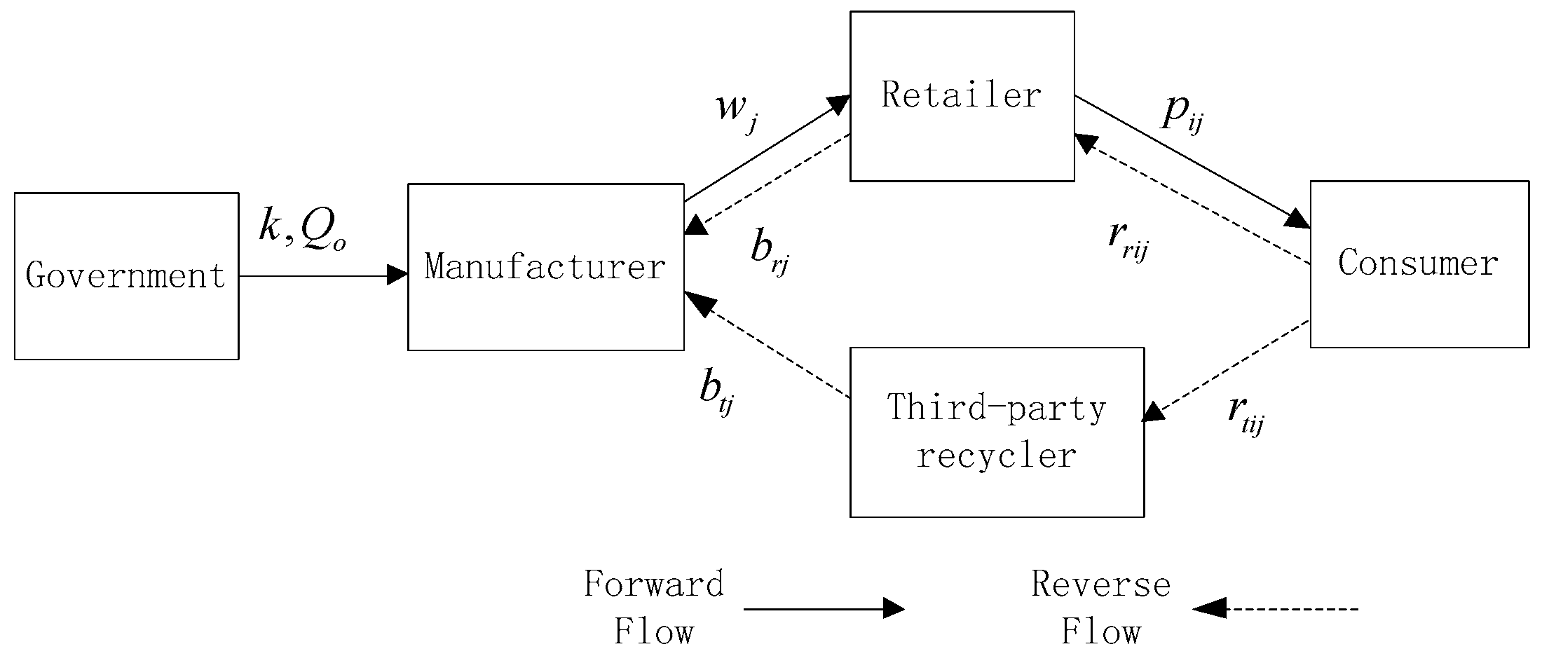
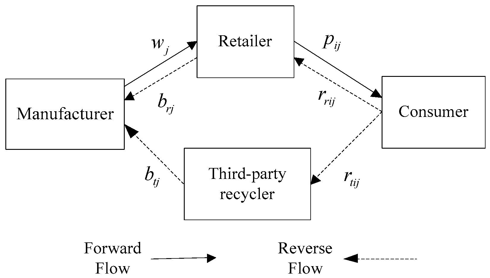
We assume the retailer’s collection quantity Q r i t j and the third-party recycler’s collection quantity Q t i r j are both collection-effort-sensitive and collection-price-sensitive. Specifically, in this paper the linear functions of Q r i t j and Q t i r j are employed by Q r i t j = e r i + r r i j ε r t i j and Q t i r j = e t i + r t i j ε r r i j respectively [23,38]. That is, for either party, collection quantity increases as the own collection effort level or collection price increases, but decreases as the competitor’s collection price increases.
In the following, we examine CLSC models without and with RPM, and compare the differences between the two models.

3. CLSC Model without the RPM (Case 1)

Figure 1 gives the general structure of CLSC without RPM, which is comprised of a manufacturer, a retailer, a third-party recycler, and consumers. The solid line and the dotted line represent the forward flow direction and the reverse flow direction, respectively. As the Stackelberg leader of CLSC, the manufacturer entrusts the retailer and the third-party recycler to collect WEEEs. According to assumptions, the two collection agents choose high or low collection effort levels separately, denoted as H-type or L-type retailers and H-type or L-type third-party recyclers. The third-party recycler collects WEEEs at the collection price r t i j from consumers, and then transfers them at buyback price b t j back to the manufacturer. The retailer acquires WEEEs at the collection price r r i j from consumers, and then resells them at buyback price b r j back to the manufacturer. The manufacturer uses recycled materials and components in preference to new materials in production owing to the lower cost. The retailer purchases new products at wholesale price w j from the manufacturer, and then sells them at the retail price p i j to final consumers. However, the real collection effort levels are only known to the retailer and the third-party recycler themselves. To enhance the efficiency of CLSC, we investigate how to design an information screening contract for the manufacturer to acquire their real private information. The decision process of the screening information is as follows: (1) the manufacturer designs information screening contracts based on the probability of being an H-type retailer or an H-type third-party recycler; (2) either the retailer or the third-party recycler chooses one contract; (3) the manufacturer identifies real collection effort levels of the two collection agents through their contract choices.

3.1. Model Description

In this section, we examine the information screening contract for the manufacturer to obtain private information from the retailer and the third-party recycler. Figure 1 shows that both the transactions of WEEEs and finished products combine the manufacturer with the retailer; only the transactions of WEEEs combine the manufacturer with the third-party recycler. So, the screening contracts designed by manufacturer for the retailer and the third-party recycler can be expressed as { G r H ( b r H , w H , T r H ) , G r L ( b r L , w L , T r L ) } and { G t H ( b t H , T t H ) , G t L ( b t L , T t L ) } , respectively.
Based on Assumptions (5) and (6), the expected profit of the manufacturer with the retailer’s choice of contract G r H and the third-party recycler’s choice of contract G t H under their real collection level H can be expressed as:
E ( π m H H ) = 0 z H H ( ϕ p H H + x ) ( w H c r ) f ( x ) d x + z H H a ( ϕ p H H + x ) ( w H c n ) f ( x ) d x + Δ z H H a [ e r H + e t H + ( 1 ε ) ( r t H H + r r H H ) ] f ( x ) d x b t H ( e t H + r t H H ε r r H H ) b r H ( e r H + r r H H ε r t H H ) + T t H + T r H ,
where z H H = e r H + e t H + ( 1 ε ) ( r t H H + r r H H ) ϕ + p H H . If 0 < x z H H , products made of recycled components can meet market demand; however, if z H H < x < a , market demand is higher than the collection quantity of WEEEs, so it is met by products made of recycled materials and new materials together.
Similarly, when the retailer chooses contract G r L under real collection level L and the third-party recycler chooses contract G t H under real collection level H , the expected profit of the manufacturer can be formulated as:
E ( π m H L ) = 0 z H L ( ϕ p L L + x ) ( w L c r ) f ( x ) d x + z H L a ( ϕ p L L + x ) ( w L c n ) f ( x ) d x + Δ z H L a [ e t H + e r L + ( 1 ε ) ( r t H H + r r L L ) ] f ( x ) d x b t H ( e t H + r t H H ε r r L L ) b r L ( e r L + r r L L ε r t H H ) + T t H + T r L ,
where z H L = e t H + e r L + ( 1 ε ) ( r t H H + r r L L ) ϕ + p L L . If 0 < x z H L , the products made of recycled components can meet market demand; however, if z H L < x < a , market demand is higher than the collection quantity of WEEEs, so it is met by products made of recycled materials and new materials together.
When the retailer chooses contract G r H under real collection level H and the third-party recycler chooses contract G t L under real collection level L , the expected profit of the manufacturer can be expressed as:
E ( π m L H ) = 0 z L H ( ϕ p H H + x ) ( w H c r ) f ( x ) d x + z L H a ( ϕ p H H + x ) ( w H c n ) f ( x ) d x + Δ z L H a [ e t L + e r H + ( 1 ε ) ( r t L L + r r H H ) ] f ( x ) d x b t L ( e t L + r t L L ε r r H H ) b r H ( e r H + r r H H ε r t L L ) + T t L + T r H ,
where z L H = e t L + e r H + ( 1 ε ) ( r t L L + r r H H ) ϕ + p H H . If 0 < x z L H , products made of recycled components can meet market demand; however, if z L H < x < a , market demand is higher than the collection quantity of WEEEs, so it is met by newly manufactured products and remanufactured products together.
When the retailer chooses contract G r L under real collection level L and the third-party recycler chooses contract G t L under real collection level L , the expected profit of the manufacturer can be formulated as:
E ( π m L L ) = 0 z L L ( ϕ p L L + x ) ( w L c r ) f ( x ) d x + z L L a ( ϕ p L L + x ) ( w L c n ) f ( x ) d x + Δ z L L a [ e t L + e r L + ( 1 ε ) ( r t L L + r r L L ) ] f ( x ) d x b t L ( e t L + r t L L ε r r L L ) b r L ( e r L + r r L L ε r t L L ) + T t L + T r L ,
where z L L = e t L + e r L + ( 1 ε ) ( r t L L + r r L L ) ϕ + p L L . If 0 < x z L L , the product made of recycled components can meet market demand; however, if z L L < x < a , market demand is higher than the collection quantity of WEEEs, hence newly manufactured products and remanufactured products together meet the market demand.
In a case where the third-party recycler adopts H collection effort level with the choice of contract G t H , her expressed profit is:
E ( π t H H ) = ( b t H r t H H ) { e t H + r t H H ε [ v r r H H + ( 1 v ) r r L L ] } e t H 2 / 4 T t H .
When the H-type third-party recycler chooses contract G t L , her expected profit is:
E ( π t H L ) = ( b t L r t H L ) { e t H + r t H L ε [ v r r H H + ( 1 v ) r r L L ] } e t H 2 / 4 T t H .
In a case where the third-party recycler adopts L collection effort level with the choice of contract G t L , her expected profit is:
E ( π t L L ) = ( b t L r t L L ) { e t L + r t L L ε [ v r r H H + ( 1 v ) r r L L ] } e t L 2 / 4 T t L .
When the L-type third-party recycler chooses contract G t H , her expected profit is:
E ( π t L H ) = ( b t H r t L H ) { e t L + r t L H ε [ v r r H H + ( 1 v ) r r L L ] } e t L 2 / 4 T t H .
In the case that the retailer makes H level collection effort with the choice of contract G r H , her expected profit is:
E ( π r H H ) = ( b r H r r H H ) { e r H + r r H H ε [ v r t H H + ( 1 v ) r t L L ] } e r H 2 / 4 + ( p H H w H ) 0 a ( ϕ p H H + x ) f ( x ) d x T r H .
If the H-type retailer chooses contract G r L , her expected profit is:
E ( π r H L ) = ( b r L r r H L ) { e r H + r r H L ε [ v r t H H + ( 1 v ) r t L L ] } e r H 2 / 4 + ( p H L w L ) 0 a ( ϕ p H L + x ) f ( x ) d x T r L .
When the retailer makes L level collection effort with the choice of contract G r L , her expected profit is:
E ( π r L L ) = ( b r L r r L L ) { e r L + r r L L ε [ v r t H H + ( 1 v ) r t L L ] } e r L 2 / 4 + ( p L L w L ) 0 a ( ϕ p L L + x ) f ( x ) d x T r L .
If the L-type retailer chooses contract G r H , her expected profit is:
E ( π r L H ) = ( b r H r r L H ) { e r L + r r L H ε [ v r t H H + ( 1 v ) r t L L ] } e r L 2 / 4 + ( p L H w H ) 0 a ( ϕ p L H + x ) f ( x ) d x T r H ,
where e t j 2 / 4 and e r j 2 / 4 denotes the cost of collection effort of the third-party recycler and the retailer, respectively.
In the CLSC without government intervention under random demand and information asymmetry, the expected profit maximization problem of the manufacturer can be expressed as:
max E ( π m ) = v 2 E ( π m H H ) + v ( 1 v ) E ( π m H L ) + v ( 1 v ) E ( π m L H ) + ( 1 v ) 2 E ( π m L L )
s . t .
r t H H * = arg max E ( π t H H )
r t L L * = arg max E ( π t L L )
r r H H * = arg max E ( π r H H )
r r L L * = arg max E ( π r L L )
p H H * = arg max E ( π r H H )
p L L * = arg max E ( π r L L )
E ( π t H H ) π t 0
E ( π t L L ) π t 0
E ( π r H H ) π r 0
E ( π r L L ) π r 0
E ( π t H H ) E ( π t H L )
E ( π t L L ) E ( π t L H )
E ( π r H H ) E ( π r H L )
E ( π r L L ) E ( π r L H ) .
The optimal profits of the retailer and the third-party recycler without contract are π r 0 and π t 0 respectively, which can be called conserved profits. Equations (20)–(23) can guarantee that the expected profits of both two collection agents are no less than their conserved profits when they accept the contract. We call these equations participation constraints.
Equations (24)–(27) indicate that both two collection agents can make the maximum profit when they choose the right contracts corresponding to their own real collection effort levels. If not, they cannot get their maximum profit. In other words, these constraint conditions avoid the third-party recycler and the retailer telling lies, so we call these constraint equations incentive compatible constraints. Specifically, Equation (24) indicates the profit of the H-type third-party recycler when the choice of contract G t H is more than that with the choice of contract G t L . Meanwhile, Equation (25) shows that the profit of the L-type third-party recycler with contract G t L is higher than that with contract G t H . Equations (26) and (27) do the same for the retailer.
It is difficult to calculate and analyze the model because it has too many constraints and its arithmetic formulas are very complicated. We will give the relevant parameters specific values, and then compute the optimal solutions with the help of a software tool of MATLAB. Finally, we will analyze the results.

3.2. Numerical Examples

To verify the efficiency of the information screening contract and analyze the competition between the two collection agents on CLSC operations without RPM, we set the parameters as follows: c n = 60 , c r = 45 , a = 4 , ϕ = 120 , e t H = e r H = 10 , e t L = e r L = 7 , π r o = 300 , π t o = 60 ; in addition, we specify v { 0.1 , 0.2 , 0.3 , 0.4 , 0.5 } , ε { 0.1 , 0.2 , 0.3 , 0.4 , 0.5 } . The optimal decision-making of CLSC with different v and ε is shown in Appendix A.
(1) We find that when ε < 0.5 , the buyback price b t H * ( b r H * ) increases as the probability v increases. When ε = 0.5 , both the buyback prices b t H * ( b r H * ) and b t L * ( b r L * ) decrease as the probability v increases. Both b t H * ( b r H * ) and b t L * ( b r L * ) decrease as the competition intensity ε increases. As shown in Figure 2, with the probability v of H level of collection effort increasing, the buyback price is not always increasing. This indicates that when the degree of collection competition between the retailer and recycler reaches a certain level, the manufacturer will still take the measure of reducing the buyback price, even if the probability v increases. This shows that competition is not advantageous to both collection agents. Buyback price under high collection effort level is always higher than that under low collection effort level when ε and v are fixed. This will make both two agents choose H level of collection effort for a higher buyback price.
(2) As shown in Figure 3 and Figure 4, the wholesale prices w H * , w L * and the retail prices p H H * , p L L * increase with the probability v and competition intensity ε . The manufacturer can get more profit by raising the wholesale prices while reducing buyback prices. Accordingly, the retailer will raise the sale price to get more profit. Wholesale price w L * is higher than w H * when ε and v are fixed. This shows that the retailer should choose H level of collection effort for a lower wholesale price and a higher buyback price.
(3) From the computing results, it can be found that the collection price of the third-party recycler is equivalent to the retailer’s, r t H H * = r r H H * , r t L L * = r r L L * . As shown in Figure 5, the collection price decreases with the increase in probability v , and first increases then decreases in competition intensity ε . To sum up, the collection price under L level of collection effort is higher than the H level of collection effort. By analyzing r t H H * , we find that when v = 0.1 , if ε 0.3 , r t H H * increases in ε ; if ε > 0.3 , r t H H * decreases in ε . When v > 0.1 , if ε 0.2 , r t H H * increases in ε ; if ε > 0.2 , r t H H * decreases in ε . Now let’s analyze r t L L * . When v 0.2 , if ε 0.3 , r t L L * increases in ε ; if ε > 0.3 , r t L L * decrease in ε . When 0.2 < v < 0.5 , if ε 0.2 , r t L L * increases in ε ; if ε > 0.2 , r t L L * decreases in ε . When v = 0.5 , if 0.1 ε 0.5 , r t L L * decreases in ε . Through an analysis of the collection price, we know that when the collection competition intensifies, the collection price will decrease. Under the situation above, when the probability of a high collection effort level is relatively small, the third-party recycler and the retailer are still able to increase the quantity of WEEEs by raising the collection price despite the buyback price falling. However, in order to deal with the buyback price reduction caused by the level of collection competition intensifying, both two collection agents will reduce the collection prices gradually.
(4) As shown in Figure 6 and Figure 7, the franchise fee T t L * and T r L * will decrease in the process of v and ε increasing; T t H * and T r H * increase in v , but decrease in ε . Therefore, in cases of competitive collection, the franchise fee charged by the manufacturer turns out to be lower when the competition becomes more intense. In addition, the franchise fee paid by the retailer is higher than that paid by the third-party recycler.
(5) When e t i = e r i , Q t H r H * = Q r H t H * , Q t L r L * = Q r L t L * ; when e t i is relatively high (or low) and e r i is relatively low (or high), Q t H r L * = Q r H t L * , Q t L r H * = Q r L t H * . According to the expression of the collection price and r t H H * = r r H H * , r t L L * = r r L L * , we can obtain the equivalence relationship between the collection quantities of the retailer and third-party recycler. Let us analyze the third-party recycler’s collection quantity. When both collection agents choose a high collection effort level, the collection quantity Q t H r H * arrives at its maximum. When both of them choose a low collection effort level, the collection quantity Q t L r L * reaches its minimum. What will happen when they choose different collection effort levels? Now we analyze the case where the third-party recycler chooses a high collection effort level and the retailer chooses a low collection effort level. When v = 0.1 , if ε < 0.2 , then Q t H r L * > Q r L t H * ; if ε > 0.2 , then Q t H r L * < Q r L t H * . When v = 0.2 , if ε 0.3 , then Q t H r L * > Q r L t H * ; if ε > 0.3 , then Q t H r L * < Q r L t H * ; when v > 0.2 , Q t H r L * > Q r L t H * regardless of ε .
From the analysis above, we can infer that even though the third-party recycler makes a high collection effort, his collection quantity is not always higher than the retailer’s. The relationship depends on the probability of a high collection effort level. For instance, in the case that the probability of high collection effort level is relatively low, e.g., v 0.2 , when the collection competition is not intense, although the third-party recycler’s collection price r t H H * is lower than that of the retailer r r L L * , the third-party recycler can still collect more WEEEs than the retailer due to her high collection effort level. However, as the collection competition intensifies the collection difficulties for both parties increase, resulting in the collection price playing a more important role than the collection effort level. So, with a more intense collection competition, a higher collection price will make the retailer collect more WEEEs than the third-party recycler despite the lower collection effort.
In the case that the probability of H collection effort level is relatively high, e.g., v > 0.2 , the effect of collection effort level outweighs that of collection price. Although the collection competition intensifies and the retailer provides a higher collection price, the third-party recycler can still acquire more WEEEs than the retailer due to her higher collection effort level. As depicted in Figure 8, the total quantity of WEEEs decreases as the collection competition intensity ε increases. When both two collection agents choose H collection effort level, the total collection quantity reaches its maximum in the case where the two parties choose different collection effort levels; the minimum will be the case where both of them choose L collection effort level.
(6) As shown in Figure 9, when the third-party recycler and retailer choose different collection effort levels, the profits of manufacturer E ( π m H H * ) , E ( π m H L * ) , E ( π m L H * ) and E ( π m L L * ) decrease in ε . E ( π m H H * ) , E ( π m H L * ) and E ( π m L H * ) increase in v . When v 0.2 , E ( π m L L * ) increases in v ; in contrast, when v > 0.2 , E ( π m L L * ) decreases in v . That is, as the collection competition intensifies, although the manufacturer raises the wholesale price and cuts the buyback price, his expected profit will shrink owing to the collection quantity decreasing. Moreover, both the expected profits of the third-party recycler and the retailer E ( π t H H * ) , E ( π r H H * ) reduce in the competition intensity ε and the probability of H collection effort level v . E ( π t L L * ) and E ( π r L L * ) always remain at the level of their reservation profits. The above results indicate that intense competition has a detrimental effect on both the retailer and the third-party recycler. Whether the two collection agents should cooperate to mitigate the negative impact of competition deserves further investigation.

4. CLSC Model with the RPM (Case 2)

With RPM, although the manufacturer still plays a leading role in CLSC, the government will take some measures to stimulate WEEEs collection. Thus, we add government intervention to the basic model. As shown in Figure 10, the government sets a target collection quantity Q 0 and the reward–penalty intensity k for the manufacturer. That is, when the total quantity of WEEEs collected by the third-party recycler and the retailer exceeds the target collection quantity, the government will reward the manufacturer for the exceeding part; otherwise, the government will penalize him for the unmet part. The intensity of reward and penalty is assumed to be the same, k , for avoiding complicated computation. The details of the information screening contract in this case are similar to those of the basic model.

4.1. Model Description

The manufacturer designs the information screening contracts similar to the basic model. The screening contracts designed for the retailer and the third-party recycler can be expressed as { G r H ( b r H , w H , T r H ) , G r L ( b r L , w L , T r L ) } and { G t H ( b t H , T t H ) , G t L ( b t L , T t L ) } , respectively. Based on their choices of the screening contracts, we can develop the model as follows:
When the third-party recycler chooses contract G t H and the retailer opts for contract G r H corresponding to their real collection level H , the expected profit of the manufacturer can be expressed as:
E ( π m H H ) = 0 z H H ( ϕ p H H + x ) ( w H c r ) f ( x ) d x + z H H a ( ϕ p H H + x ) ( w H c n ) f ( x ) d x + Δ z H H a [ e t H + e r H + ( 1 ε ) ( r t H H + r r H H ) ] f ( x ) d x b t H ( e t H + r t H H ε r r H H ) b r H ( e r H + r r H H ε r t H H ) + T t H + T r H + k [ e t H + e r H + ( 1 ε ) ( r t H H + r r H H ) Q 0 ] ,
where z H H = e t H + e r H + ( 1 ε ) ( r t H H + r r H H ) ϕ + p H H . If 0 < x z H H , the remanufactured products made of recycled components can meet market demand; however, if z H H < x < a , market demand exceeds the collection quantity of WEEEs, it is met by products made of recycled materials and new materials together.
Similarly, when the third-party recycler opts for contract G t H with her real collection level H and the retailer chooses contract G r L under her real collection level L , the expected profit of the manufacturer can be formulated as:
E ( π m H L ) = 0 z H L ( ϕ p L L + x ) ( w L c r ) f ( x ) d x + z H L a ( ϕ p L L + x ) ( w L c n ) f ( x ) d x + Δ z H L a [ e t H + e r L + ( 1 ε ) ( r t H H + r r L L ) ] f ( x ) d x b t H ( e t H + r t H H ε r r L L ) b r L ( e r L + r r L L ε r t H H ) + T t H + T r L + k [ e t H + e r L + ( 1 ε ) ( r t H H + r r L L ) Q 0 ] ,
where z H L = e t H + e r L + ( 1 ε ) ( r t H H + r r L L ) ϕ + p L L . If 0 < x < z H L , the remanufactured products are enough to meet market demand; however, if z H L < x < a , market demand exceeds the collection quantity of WEEEs, so it is met by the newly manufactured products and remanufactured products together.
When the third-party recycler chooses contract G t L with her real collection level L and the retailer opts for contract G r H with her real collection level H , the expected profit of manufacturer can be formulated as:
E ( π m L H ) = 0 z L H ( ϕ p H H + x ) ( w H c r ) f ( x ) d x + z L H a ( ϕ p H H + x ) ( w H c n ) f ( x ) d x + Δ z L H a [ e t L + e r H + ( 1 ε ) ( r t L L + r r H H ) ] f ( x ) d x b t L ( e t L + r t L L ε r r H H ) b r H ( e r H + r r H H ε r t L L ) + T t L + T r H + k [ e t L + e r H + ( 1 ε ) ( r t L L + r r H H ) Q 0 ] ,
where z L H = e t L + e r H + ( 1 ε ) ( r t L L + r r H H ) ϕ + p H H . If 0 < x z L H , the remanufactured products can meet the market demand; however, if z L H < x < a , the market demand exceeds the collection quantity of WEEEs, so it is met by the new-manufactured products and remanufactured products together.
When the third-party recycler chooses contract G t L with her real collection level L and the retailer chooses contract G r L under her real collection level L , the expected profit of the manufacturer can be expressed as:
E ( π m L L ) = 0 z L L ( ϕ p L L + x ) ( w L c r ) f ( x ) d x + z L L a ( ϕ p L L + x ) ( w L c n ) f ( x ) d x + Δ z L L a [ e t L + e r L + ( 1 ε ) ( r t L L + r r L L ) ] f ( x ) d x b t L ( e t L + r t L L ε r r L L ) b r L ( e r L + r r L L ε r t L L ) + T t L + T r L + k [ e t L + e r L + ( 1 ε ) ( r t L L + r r L L ) Q 0 ] ,
where z L L = e t L + e r L + ( 1 ε ) ( r t L L + r r L L ) ϕ + p L L . If 0 < x z L L , the remanufactured products can meet market demand; however, if z L L < x < a , market demand exceeds the collection quantity of WEEEs, so newly manufactured products and remanufactured products together satisfy the market demand.
In a case where the third-party recycler with collection effort level H chooses contract G t H , her expected profit is given as follows:
E ( π t H H ) = ( b t H r t H H ) { e t H + r t H H ε [ v r r H H + ( 1 v ) r r L L ] } e t H 2 4 T t H .
When the H-type third-party recycler chooses contract G t L , her expected profit can be formulated as:
E ( π t H L ) = ( b t L r t H L ) { e t H + r t H L ε [ v r r H H + ( 1 v ) r r L L ] } e t H 2 4 T t L .
In a case where the third-party recycler with collection effort level L opts for contract GtL, her expected profit is given as follows:
E ( π t L L ) = ( b t L r t L L ) { e t L + r t L L ε [ v r r H H + ( 1 v ) r r L L ] } e t L 2 4 T t L .
When the L-type third-party recycler chooses contract G t H , her expected profit can be formulated as:
E ( π t L H ) = ( b t H r t L H ) { e t L + r t L H ε [ v r r H H + ( 1 v ) r r L L ] } e t L 2 4 T t H .
When the retailer makes H level collection effort with the choice of contract G r H , her expected profit is given as follows:
E ( π r H H ) = ( b r H r r H H ) { e r H + r r H H ε [ v r t H H + ( 1 v ) r t L L ] } e r H 2 4 + ( p H H w H ) 0 a ( ϕ p H H + x ) f ( x ) d x T r H .
If the H-type retailer opts for contract G r H , her expected profit can be expressed as:
E ( π r H L ) = ( b r L r r H L ) { e r H + r r H L ε [ v r t H H + ( 1 v ) r t L L ] } e r H 2 4 + ( p H L w L ) 0 a ( ϕ p H L + x ) f ( x ) d x T r L .
When the retailer makes L level collection effort with the choice of contract G r L , her expected profit is given as follows:
E ( π r L L ) = ( b r L r r L L ) { e r L + r r L L ε [ v r t H H + ( 1 v ) r t L L ] } e r L 2 4 + ( p L L w L ) 0 a ( ϕ p L L + x ) f ( x ) d x T r L .
If the L-type retailer opts for contract G r H , her expected profit can be expressed as:
E ( π r L H ) = ( b r H r r L H ) { e r L + r r L H ε [ v r t H H + ( 1 v ) r t L L ] } e r L 2 4 + ( p L H w H ) 0 a ( ϕ p L H + x ) f ( x ) d x T r H .
In the CLSC with RPM imposed on the manufacturer by government under random demand and information asymmetry, the expected profit maximization problem of the manufacturer can be formulated as follows:
max E ( π m ) = v 2 E ( π m H H ) + v ( 1 v ) E ( π m H L ) + v ( 1 v ) E ( π m L H ) + ( 1 v ) 2 E ( π m L L )
s . t .
r t H H * * = arg max E ( π t H H )
r t L L * * = arg max E ( π t L L )
r r H H * * = arg max E ( π r H H )
r r L L * * = arg max E ( π r L L )
p H H * * = arg max E ( π r H H )
p L L * * = arg max E ( π r L L )
E ( π t H H ) π t 0
E ( π t L L ) π t 0
E ( π r H H ) π r 0
E ( π r L L ) π r 0
E ( π t H H ) E ( π t H L )
E ( π t L L ) E ( π t L H )
E ( π r H H ) E ( π r H L )
E ( π r L L ) E ( π r L H ) .
Equations (47)–(50) are participation constraints. These equations ensure that the expected profits of both two collection agents are no less than their conserved profits if they accept the contract. Equations (51)–(54) are incentive compatibility constraints, which ensure that both two collection agents will get higher profits when they select the same type contracts as their real collection effort levels.
We will give the relevant parameters specific values and compute these optimal solutions with the aid of a software tool of MATLAB.

4.2. Numerical Example

We assumed that c n = 60 , c r = 45 , a = 4 , ϕ = 120 , e t H = e r H = 10 , e t L = e r L = 7 , π r o = 300 , π t o = 60 , Δ = c n c r , v = 0.5 ; moreover, we specify ε { 0.1 , 0.2 , 0.3 , 0.4 , 0.5 } , k { 10 , 20 , 30 , 40 } and Q 0 = 32 . The optimal decisions of this model (given in Appendix B) vary when the competition intensity ε and the reward–penalty intensity k have different values.
(1) As shown in Figure 11, Figure 12 and Figure 13, we know that both the buyback prices b H * * and b L * * , all the collection prices r t H H * * , r r H H * * , r t L L * * and r r L L * * , and all the collection quantities Q t H r H * * , Q r H t H * * , Q t H r L * * , Q r H t L * * , Q t L r H * * , Q r L t H * * , Q t L r L * * and Q r L t L * * increase in the reward–penalty intensity k , while r t H H * * = r r H H * * , r t L L * * = r r L L * * and Q t H r H * * = Q r H t H * * , Q t H r L * * = Q r H t L * * , Q t L r H * * = Q r L t H * * , Q t L r L * * = Q r L t L * * . So, in a case where collection competition exists, the total collection quantity of the two collection agents will increase in the reward–penalty intensity with RPM. From these figures, we also see the relationship between these parameters: buyback price, collection price, collection quantity, the reward–penalty intensity, and competition intensity. When both the third-party recycler and the retailer choose collection effort level H , their own collection quantities Q t H r H * * and Q r H t H * * will be the highest. In contrast, when both choose collection effort level L , their collection quantities Q t L r L * * and Q r L t L * * will be the least. When one of them chooses collection effort level H while the other chooses collection effort level L , the one choosing H can collect more WEEEs than the other choosing L . By comparison with the results in Appendix A, the buyback prices with RPM are higher than without RPM, i.e., b H * * > b H * , b L * * > b L * . It is the same with the collection prices and collection quantities, namely r t H H * * > r t H H * , r t L L * * > r t L L * , r r H H * * > r r H H * , r r L L * * > r r L L * and Q t H r H * * > Q t H r H * , Q t H r L * * > Q t H r L * , Q t L r H * * > Q t L r H * , Q t L r L * * > Q t L r L * , Q r H t H * * > Q r H t H * , Q r H t L * * > Q r H t L * , Q r L t H * * > Q r L t H * , Q r L t L * * > Q r L t L * . The RPM makes the manufacturer raise the buyback prices, and then both the collection agents increase the collection prices accordingly. So, the collection quantities are boosted.
(2) As shown in Figure 14 and Figure 15, the wholesale prices w H * * and w L * * , and the retail prices p H H * * and p L L * * decrease in the reward–penalty intensity k . By comparison with the results in Appendix A, the wholesale prices with RPM are lower than without RPM, i.e., w H * * < w H * , w L * * < w L * . It is the same with the retail prices, namely p H H * * < p H H * and p L L * * < p L L * .
(3) As shown in Figure 16 and Figure 17, the franchise fees T t H * * and T t L * * of the third-party recycler and T r H * * and T r L * * of the retailer charged by the manufacturer increase in the reward–penalty intensity k . By comparison with the results of Appendix A, we see that the franchise fees charged by the manufacturer on the two collection agents with RPM are more than without RPM, i.e., T t H * * > T t H * , T t L * * > T t L * , T r H * * > T r H * , T r L * * > T r L * . In addition, the manufacturer can get more profit by raising the franchise fee under RPM.
(4) As shown in Figure 18, as the reward–penalty intensity k increases, the expected profits of the manufacturer E ( π m H H * * ) , E ( π m H L * * ) , E ( π m L H * * ) and E ( π m L L * * ) first decrease, then increase. Specifically, when ε 0.3 , if k 20 , the expected profit of the manufacturer decreases in the reward–penalty intensity k ; but if k > 20 , his expected profit increases in k . When ε = 0.4 , if k 30 , his expected profit decreases with k rising; if k > 30 , the changing trend of his expected profit is just the opposite. When ε 0.5 , his expected profit is always decreasing with k rising. We can deduce that under moderate collection competition intensity between the third-party recycler and the retailer, there is a large enough reward–penalty intensity to make the manufacturer better off. However, in the case without RPM, the manufacturer’s expected profits always decrease as the competition intensity rises. Therefore, the RPM can motivate the manufacturer, which serves as the leader of the CLSC, to collect more WEEEs via the retailer and the third-party recycler.
By comparing the manufacturer’s expected profits under RPM with those in the absence of RPM, we find that when ε 0.2 , if k 30 , E ( π m H H * * ) < E ( π m H H * ) , E ( π m H L * * ) < E ( π m H L * ) , E ( π m L L * * ) < E ( π m L L * ) ; if k > 30 , E ( π m H H * * ) > E ( π m H H * ) , E ( π m H L * * ) > E ( π m H L * ) , E ( π m L L * * ) > E ( π m L L * ) . When ε > 0.2 , E ( π m H H * * ) < E ( π m H H * ) , E ( π m H L * * ) < E ( π m H L * ) , E ( π m L L * * ) < E ( π m L L * ) .
In the model with RPM, we find that in order to improve the expected profit of the manufacturer, a larger reward–penalty intensity is needed as the collection competition intensifies. This is because, with the increase of the reward–penalty intensity, the quantity of WEEEs collected by the third-party recycler and the retailer is lower than the target collection quantity to start with, and then turns out to be higher than the target collection quantity. When the collection quantity is lower than the target collection quantity, the manufacturer will be penalized, and thus the expected profit is lower than without RPM; on the contrary, when the collection quantity is higher than the target collection quantity, the manufacturer will be rewarded, and thus the expected profit is higher than without RPM.
(5) The expected profit of the third-party recycler E ( π t H H * * ) and the expected profit of the retailer E ( π t H H * * ) increase in reward–penalty intensity when both of them choose collection effort level H , while their expected profits are equal to the conserved profits when they choose collection effort level L . By comparison with the results in Appendix A, the expected profits of the two collection agents with RPM are higher than without RPM when they choose collection effort level H , i.e., E ( π t H H * * ) > E ( π t H H * ) , E ( π r H H * * ) > E ( π r H H * ) ; when they choose collection effort level L , their expected profits with RPM are equal to without RPM, which are their conserved profits, i.e., E ( π t L L * * ) = E ( π t L L * ) = π t 0 , E ( π r L L * * ) = E ( π r L L * ) = π r 0 .

5. Conclusions and Future Research

In this paper, we study a CLSC with dual collection channel, in which the manufacturer entrusts one retailer and one third-party recycler with collecting WEEEs in competition. The collection effort levels of both collection agents are only known to themselves. The manufacturer provides information screening contracts for the two collection agents in order to attain real information about their collection effort levels. In this context, we focus on verifying the efficiency of the information screening contracts and exploring the influence of the RPM on the CLSC with competitive dual collection channel and information asymmetry. The contract parameters and optimal decision-making results are obtained by numerical simulation and the main findings are as follows:
(1)
The information screening contract can help the manufacturer acquire the real collection effort levels effectively because the two collection agents are induced to choose the same type of contract as their collection effort type for profit maximization. That is, the screening contract can prevent them from lying and improve the efficiency of the CLSC system.
(2)
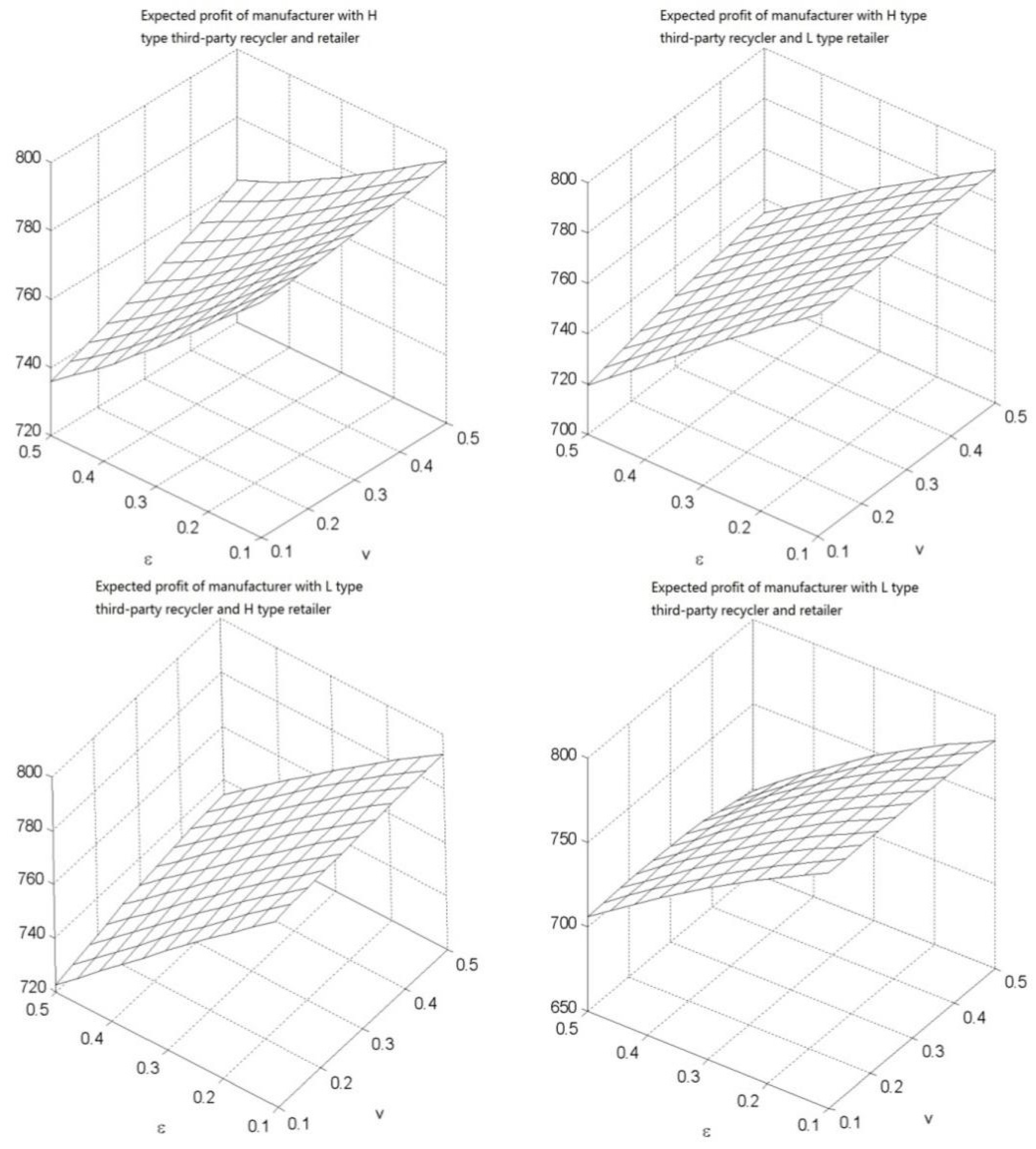
The retailer and the third-party recycler will earn more profit by choosing a high level collection effort when competing against each other. The collection competition reduces the total collection quantity and the expected profit of the manufacturer, while the expected profits of both two collection agents first increase and then decrease as the competition intensity increases. In addition, the more intense the collection competition is, the more losses they will suffer. Therefore, the CLSC channel members should make efforts to come to a cooperation agreement for mitigating the negative effect of the competition.
(3)
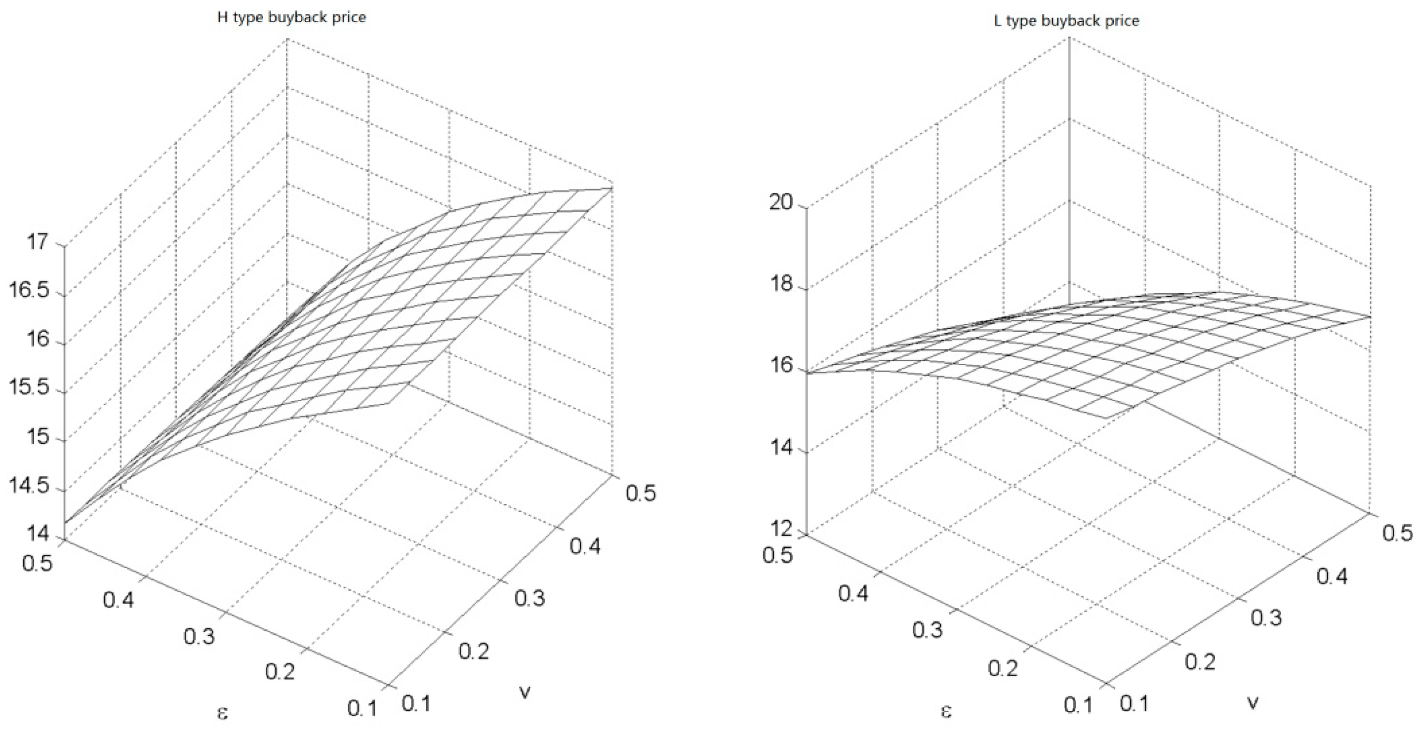
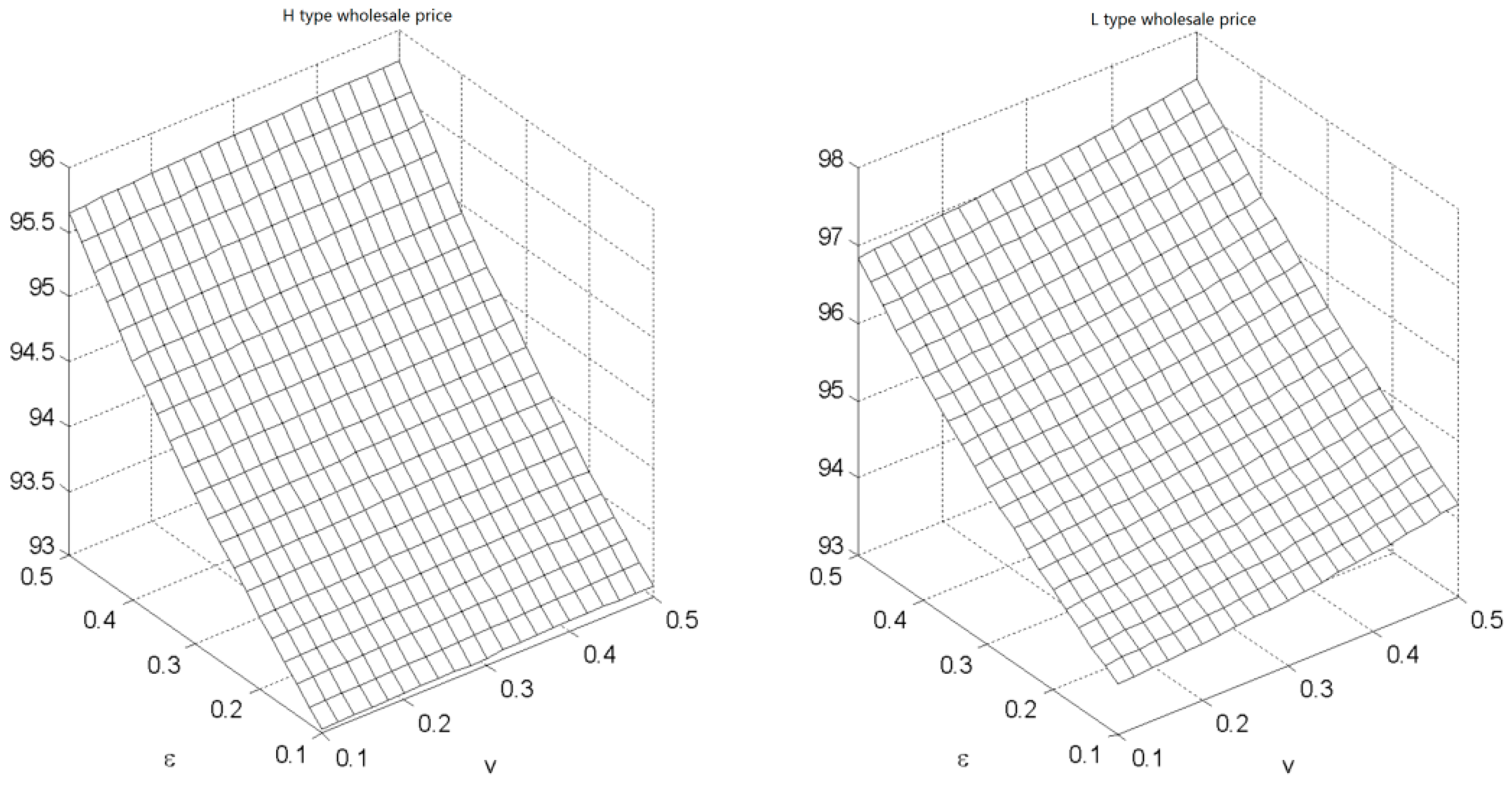
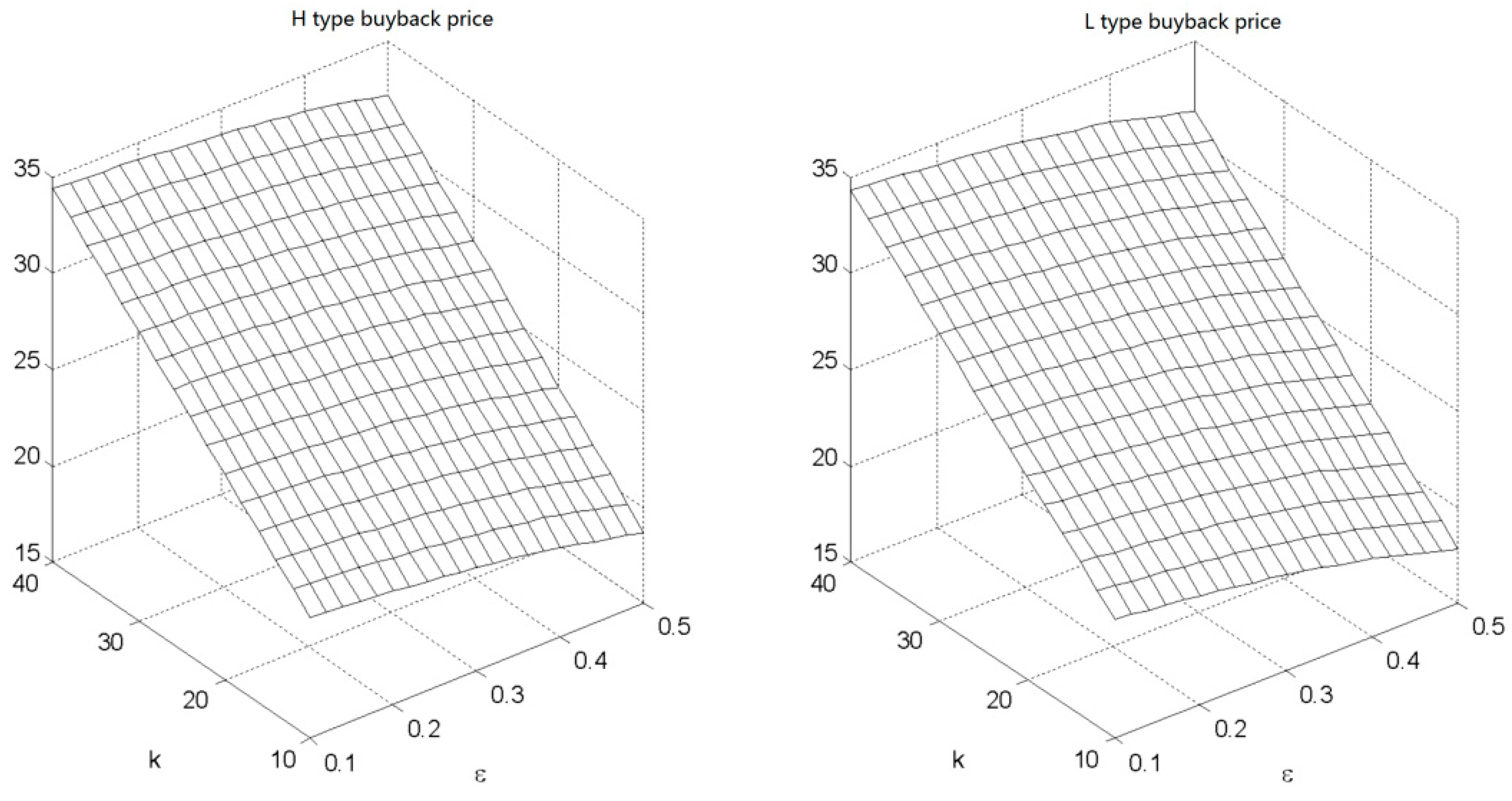
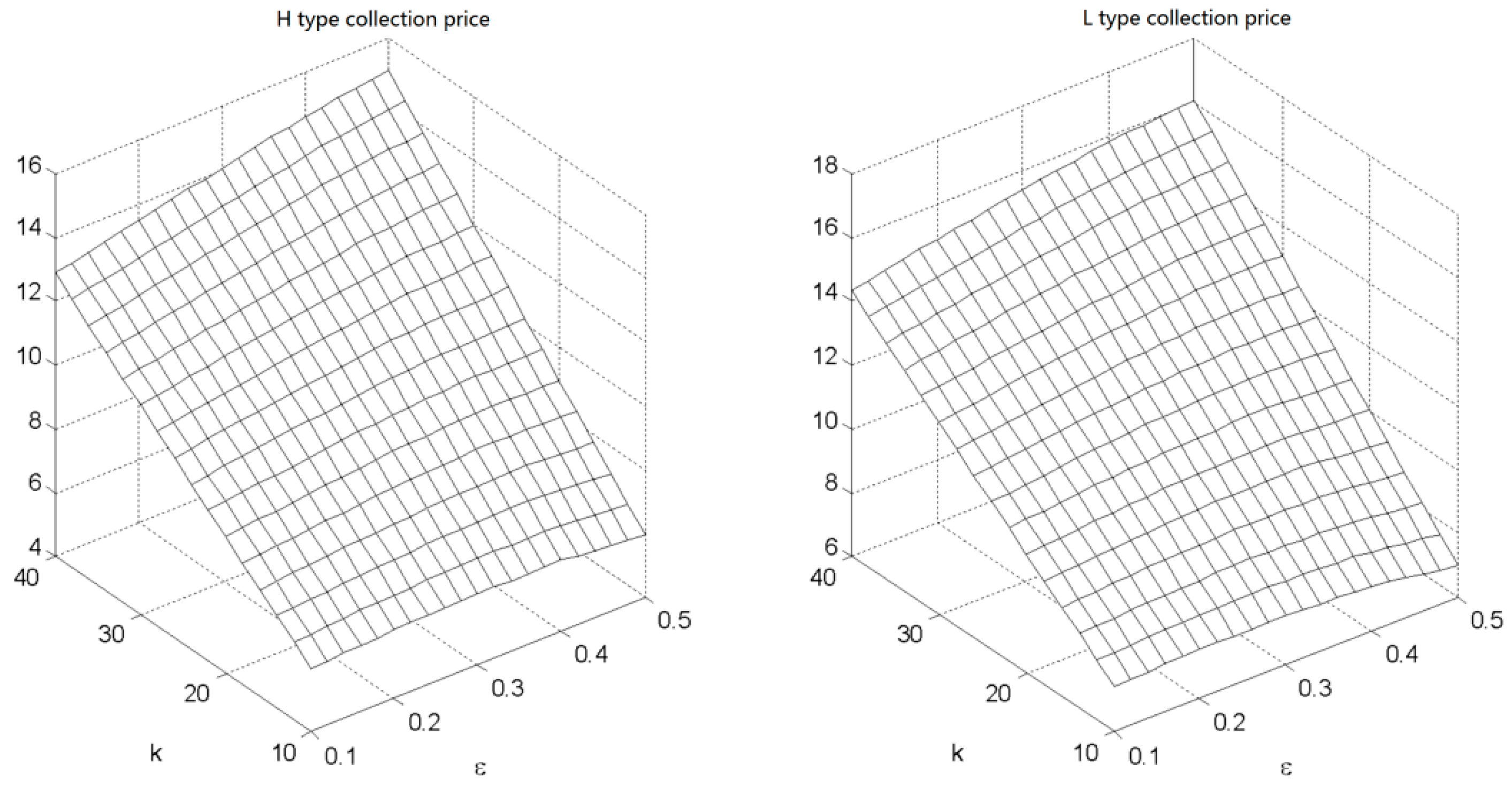
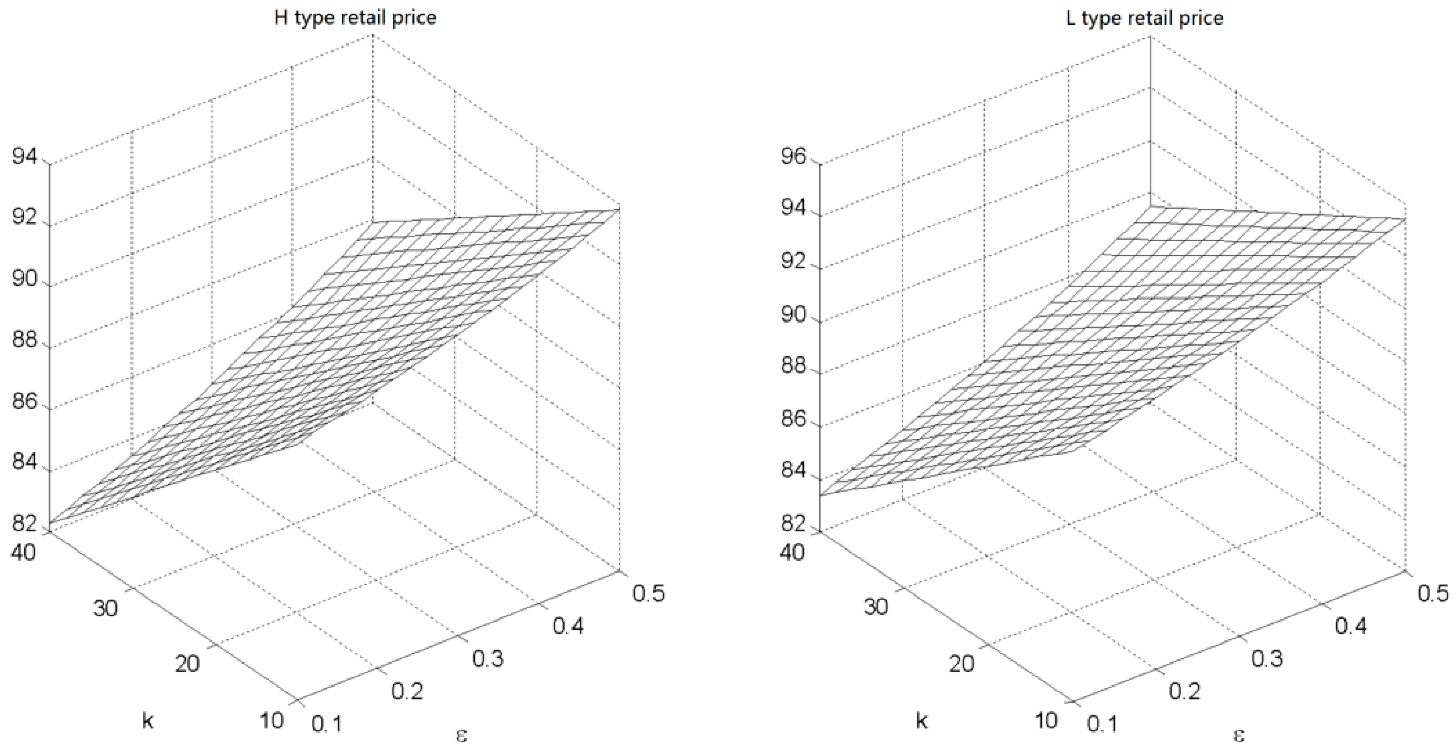
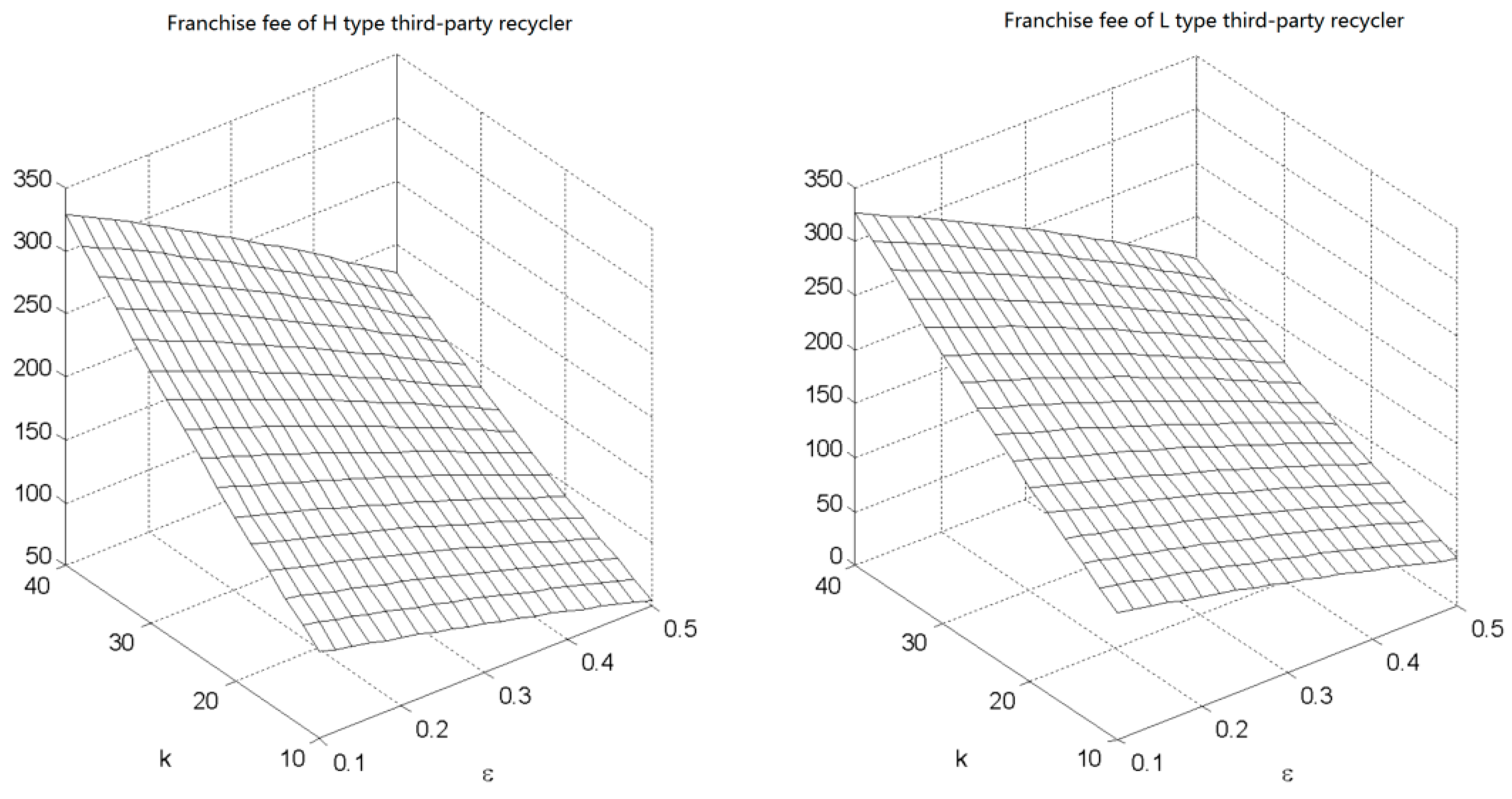
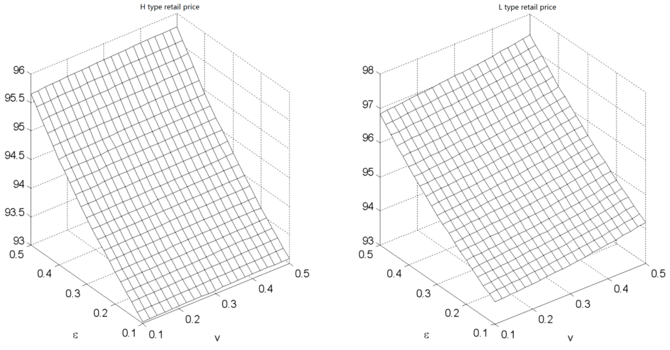
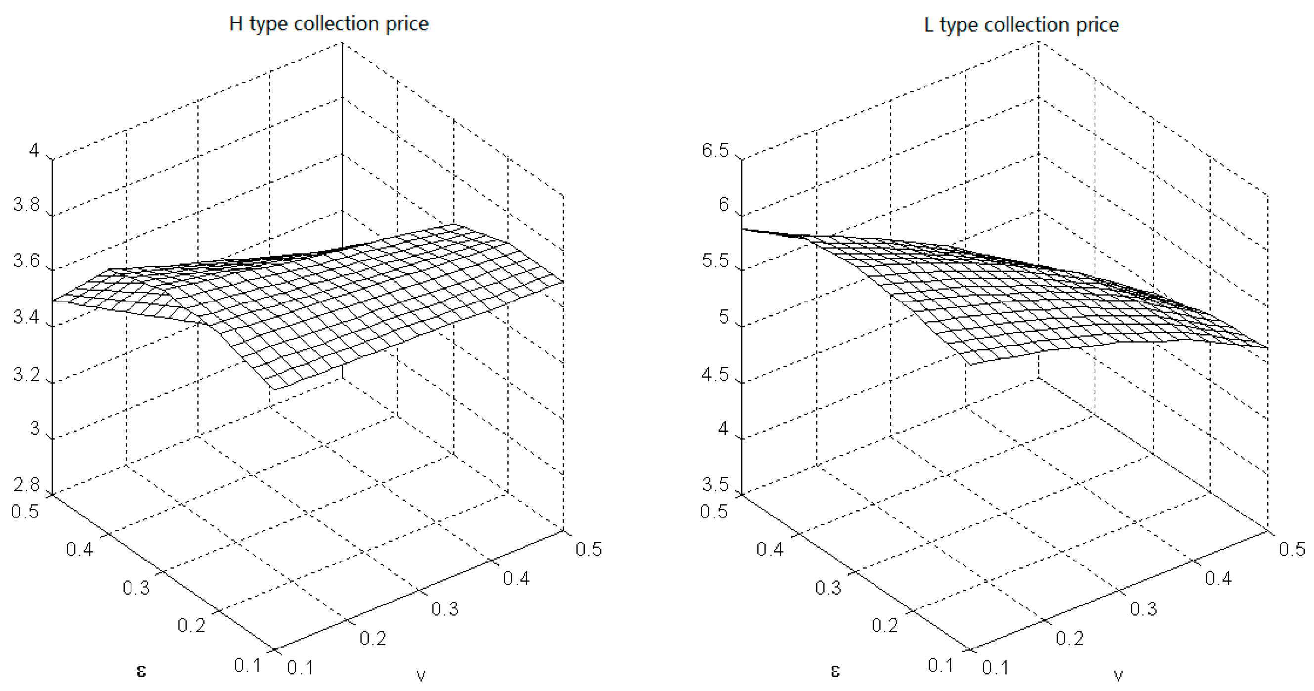
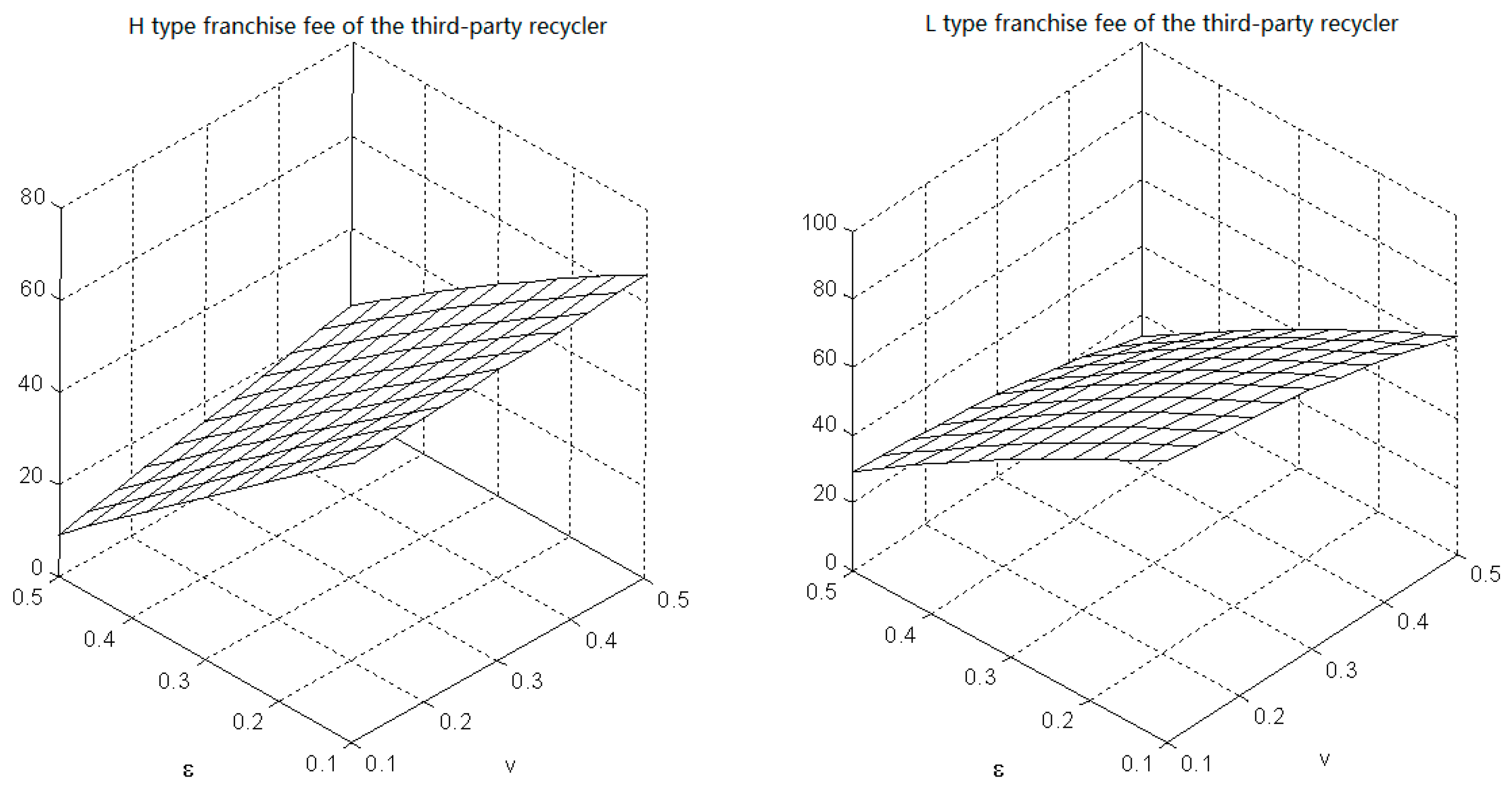
The RPM has a positive effect on CLSC with collection competition. First, RPM increases the collection price, buyback price, franchise fee, and total collection quantity; secondly, it can encourage initiatives of the collectors in collecting WEEEs, and then the environmental benefits to society will improve. What is more, the RPM can ensure that the profits of all the CLSC members are superior to without RPM.
This paper is among the first efforts to investigate the impact of RPM on a CLSC with competitive dual collection channel and information asymmetry. Several possible extensions deserve future research. First, all the conclusions we have obtained are based on a case where the manufacturer delegates the collection task to the mutual competitive retailer and third-party recycler. However, as Savaskan et al. [5] have noted, the manufacturer may choose to collect the WEEEs itself. So, other competition forms, such as mutual competitive manufacturer and retailer (or mutual competitive manufacturer and the third-party recycler) can also be examined. Secondly, we assume that there is no difference between the new product and the remanufactured product. In reality, however, there are many differences between the two types of products. For instance, the price of a remanufactured product may be lower than that of a new product, so the product differentiation needs to be considered in the future. Finally, this paper assumes that all the CLSC members are risk-neutral and profit maximizers. We may need to incorporate the risk attitudes of the decision-makers into the CLSC model.

Author Contributions

Conceptualization, W.W. and L.H.; Formal analysis, W.W. and S.Z.; Investigation, S.Z. and M.Z.; Writing—original draft, S.Z. and M.Z.; Writing—review & editing, H.S.; Funding acquisition, H.S.

Funding

This research was funded by the Postgraduate Education & Teaching Reform Research & Practice Innovation Program of Jiangsu Province (No. JGLX16_064) and the Natural Science Foundation of Shandong Province of China (ZR2017MG015).

Conflicts of Interest

The authors declare no conflict of interests.

Appendix A

Table A1. The optimal CLSC decision results vs. v and ε without RPM.
ε v
0.10.20.30.40.5
b r H * , b t H *
0.116.87016.89016.91016.92016.940
0.216.39016.42016.45016.48016.510
0.315.82015.86015.89015.93015.960
0.415.12015.14015.17015.19015.210
0.514.17014.16014.15014.13014.120
b r L * , b t L *
0.118.510 18.250 17.920 17.470 16.830
0.218.150 17.860 17.490 17.000 16.300
0.317.660 17.330 16.910 16.360 15.590
0.416.960 16.580 16.100 15.470 14.620
0.515.940 15.480 14.910 14.190 13.230
w H *
0.164.070 64.090 64.120 64.150 64.180
0.265.120 65.160 65.190 65.230 65.260
0.366.320 66.370 66.410 66.450 66.480
0.467.700 67.760 67.810 67.850 67.890
0.569.300 69.380 69.440 69.500 69.540
w L *
0.165.260 65.450 65.680 65.990 66.400
0.266.550 66.760 67.000 67.300 67.720
0.368.030 68.240 68.490 68.790 69.190
0.469.710 69.930 70.180 70.480 70.860
0.571.660 71.880 72.130 72.410 72.770
r t H H *
0.13.726 3.718 3.711 3.698 3.691
0.23.788 3.764 3.740 3.717 3.694
0.33.808 3.763 3.713 3.670 3.622
0.43.744 3.656 3.575 3.490 3.407
0.53.496 3.349 3.205 3.059 2.922
r t L L *
0.16.046 5.898 5.716 5.473 5.136
0.26.168 5.984 5.760 5.477 5.089
0.36.228 5.998 5.723 5.385 4.937
0.46.164 5.876 5.540 5.130 4.612
0.55.880 5.509 5.085 4.589 3.978
r r H H *
0.13.726 3.718 3.711 3.698 3.691
0.23.788 3.764 3.740 3.717 3.694
0.33.808 3.763 3.713 3.670 3.622
0.43.744 3.656 3.575 3.490 3.407
0.53.496 3.349 3.205 3.059 2.922
r r L L *
0.16.046 5.898 5.716 5.473 5.136
0.26.168 5.984 5.760 5.477 5.089
0.36.228 5.998 5.723 5.385 4.937
0.46.164 5.876 5.540 5.130 4.612
0.55.880 5.509 5.085 4.589 3.978
p H H *
0.193.035 93.045 93.060 93.080 93.090
0.293.560 93.580 93.600 93.620 93.630
0.394.160 94.180 94.200 94.220 94.240
0.494.850 94.880 94.900 94.920 94.940
0.595.650 95.690 95.720 95.750 95.770
p L L *
0.193.630 93.720 93.840 94.000 94.200
0.294.280 94.380 94.500 94.650 94.860
0.395.020 95.120 95.240 95.400 95.600
0.495.860 95.960 96.090 96.240 96.430
0.596.830 96.940 97.060 97.200 97.380
T t H *
0.160.880 61.943 63.108 64.326 65.961
0.248.364 50.046 51.846 53.819 56.113
0.335.494 37.849 40.218 42.886 45.769
0.422.517 25.262 28.262 31.374 34.789
0.59.269 12.460 15.814 19.259 23.127
T t L *
0.183.109 80.319 76.694 71.674 64.507
0.271.318 68.789 65.334 60.523 53.433
0.358.443 56.172 52.899 48.204 41.238
0.444.295 42.317 39.261 34.670 27.912
0.528.946 27.166 24.276 19.924 13.359
T r H *
0.1659.860 660.340 660.630 660.980 661.750
0.2617.190 617.740 618.690 619.530 620.970
0.3570.560 571.530 572.780 574.340 576.380
0.4519.640 520.760 522.400 524.430 526.760
0.5463.590 464.680 466.450 468.330 471.140
T r L *
0.1647.970 639.800 629.680 615.950 597.350
0.2599.990 591.650 581.580 568.550 550.010
0.3546.630 538.710 528.730 516.030 498.460
0.4487.860 480.140 470.590 458.250 441.740
0.5422.470 415.170 406.030 394.720 379.260
Q t H r H * , Q r H t H *
0.113.353 13.346 13.340 13.330 13.320
0.213.030 13.011 12.992 12.974 12.955
0.312.666 12.634 12.599 12.569 12.535
0.412.246 12.194 12.145 12.094 12.044
0.511.748 11.674 11.602 11.530 11.461
Q t H r L * , Q r H t L *
0.113.120 13.130 13.140 13.150 13.180
0.212.550 12.570 12.590 12.620 12.680
0.311.940 11.960 12.000 12.050 12.140
0.411.280 11.310 11.360 11.440 11.560
0.510.560 10.590 10.660 10.760 10.930
Q t L r H * , Q r L t H *
0.112.670 12.530 12.340 12.100 11.770
0.212.410 12.230 12.010 11.730 11.350
0.312.090 11.870 11.610 11.280 10.850
0.411.670 11.410 11.110 10.730 10.250
0.511.130 10.830 10.480 10.060 9.517
Q t L r L * , Q r L t L *
0.112.440 12.310 12.140 11.930 11.620
0.211.930 11.790 11.610 11.380 11.070
0.311.360 11.200 11.010 10.770 10.460
0.410.700 10.530 10.320 10.080 9.767
0.59.940 9.754 9.542 9.294 8.989
Q t H r H * + Q r H t H *
0.126.710 26.690 26.680 26.660 26.640
0.226.060 26.020 25.980 25.950 25.910
0.325.330 25.270 25.200 25.140 25.070
0.424.490 24.390 24.290 24.190 24.090
0.523.500 23.350 23.200 23.060 22.920
Q t H r L * + Q r H t L * , Q t L r H * + Q r L t H *
0.125.790 25.650 25.480 25.250 24.940
0.224.960 24.800 24.600 24.360 24.030
0.324.030 23.830 23.610 23.340 22.990
0.422.940 22.720 22.470 22.170 21.810
0.521.690 21.430 21.140 20.820 20.450
Q t L r L * + Q r L t L *
0.124.880 24.620 24.290 23.850 23.240
0.223.870 23.570 23.220 22.760 22.140
0.322.720 22.400 22.010 21.540 20.910
0.421.400 21.050 20.650 20.160 19.530
0.519.880 19.510 19.080 18.590 17.980
E ( π m H H * )
0.1788.550 790.150 791.890 794.010 796.730
0.2774.670 777.180 779.930 783.020 786.790
0.3760.750 764.290 768.090 772.260 777.080
0.4747.460 752.050 756.950 762.290 768.220
0.5736.050 741.810 747.900 754.370 761.460
E ( π m H L * )
0.1788.440 789.610 790.740 791.810 792.760
0.2772.310 774.310 776.240 778.020 779.420
0.3755.130 758.050 760.790 763.190 765.070
0.4737.300 741.090 744.570 747.640 749.890
0.5719.400 724.050 728.330 731.940 734.420
E ( π m L H * )
0.1789.270 790.390 791.440 792.320 792.760
0.2773.500 775.420 777.180 778.650 779.430
0.3756.840 759.570 761.990 763.990 765.070
0.4739.650 743.100 746.180 748.600 749.850
0.5722.600 726.770 730.390 733.130 734.410
E ( π m L L * )
0.1788.820 789.050 788.830 787.780 785.000
0.2771.260 771.880 771.820 770.650 767.330
0.3751.710 752.630 752.620 751.190 747.160
0.4729.930 731.020 730.950 729.060 724.230
0.5705.920 707.040 706.680 704.220 698.430
E ( π t H H * )
0.186.893 86.556 86.113 85.491 84.584
0.285.446 85.128 84.688 84.068 83.133
0.383.797 83.497 83.061 82.425 81.459
0.481.887 81.611 81.180 80.521 79.524
0.579.678 79.412 78.974 78.303 77.257
E ( π t L L * )
0.160.000 60.000 60.000 60.000 60.000
0.260.000 60.000 60.000 60.000 60.000
0.360.000 60.000 60.000 60.000 60.000
0.460.000 60.000 60.000 60.000 60.000
0.560.000 60.000 60.000 60.000 60.000
E ( π r H H * )
0.1326.880 326.550 326.110 325.490 324.580
0.2325.450 325.130 324.690 324.060 323.130
0.3323.800 323.490 323.060 322.420 321.470
0.4321.890 321.610 321.180 320.520 319.530
0.5319.680 319.410 318.980 318.290 317.260
E ( π r L L * )
0.1300.000 300.000 300.000 300.000 300.000
0.2300.000 300.000 300.000 300.000 300.000
0.3300.000 300.000 300.000 300.000 300.000
0.4300.000 300.000 300.000 300.000 300.000
0.5300.000 300.000 300.000 300.000 300.000

Appendix B

Table A2. The optimal CLSC decision results vs. k and ε with RPM.
k ε
0.10.20.30.40.5
b t H * * , b r H * *
1021.310 20.920 20.400 19.700 18.660
2025.680 25.320 24.850 24.180 23.190
3030.050 29.730 29.290 28.670 27.730
4034.420 34.130 33.730 33.160 32.270
b t L * * , b r L * *
1021.200 20.700 20.030 19.100 17.770
2025.570 25.110 24.480 23.590 22.310
3029.940 29.510 28.920 28.080 26.850
4034.310 33.920 33.360 32.570 31.390
w H * *
1058.780 60.150 61.710 63.500 65.590
2053.380 55.040 56.940 59.110 61.650
3047.980 49.940 52.160 54.720 57.700
4042.580 44.830 47.390 50.330 53.750
w L * *
1061.000 62.610 64.420 66.470 68.820
2055.600 57.500 59.650 62.080 64.870
3050.200 52.400 54.880 57.690 60.920
4044.800 47.290 50.100 53.300 56.980
r t H H * *
105.991 6.144 6.234 6.212 5.949
208.291 8.589 8.851 9.013 8.970
3010.590 11.040 11.460 11.820 12.000
4012.890 13.480 14.070 14.630 15.020
r t L L * *
107.436 7.534 7.549 7.412 7.004
209.736 9.984 10.170 10.220 10.030
3012.040 12.430 12.780 13.020 13.060
4014.340 14.880 15.390 15.830 16.080
r r H H * *
105.991 6.144 6.234 6.212 5.949
208.291 8.589 8.851 9.013 8.970
3010.590 11.040 11.460 11.820 12.000
4012.890 13.480 14.070 14.630 15.020
r r L L * *
107.436 7.534 7.549 7.412 7.004
209.736 9.984 10.170 10.220 10.030
3012.040 12.430 12.780 13.020 13.060
4014.340 14.880 15.390 15.830 16.080
p H H * *
1090.390 91.080 91.860 92.750 93.800
2087.690 88.520 89.470 90.560 91.820
3084.990 85.970 87.080 88.360 89.850
4082.290 83.420 84.700 86.160 87.880
p L L * *
1091.500 92.300 93.210 94.240 95.410
2088.800 89.750 90.820 92.040 93.440
3086.100 87.200 88.440 89.840 91.460
4083.400 84.640 86.050 87.650 89.490
T t H * *
10118.890 104.340 88.739 72.353 54.769
20180.390 160.060 138.510 115.410 90.868
30250.450 223.630 194.870 164.290 131.630
40329.090 294.670 257.930 218.790 177.050
T t L * *
10117.210 101.100 83.532 64.350 43.654
20178.480 156.560 132.620 106.550 78.548
30248.310 219.530 188.310 154.430 117.980
40326.720 290.350 250.690 207.940 162.070
T r H * *
10878.080 820.690 757.460 687.920 610.290
201117.500 1041.000 956.710 864.200 761.400
301380.200 1281.800 1174.300 1055.900 925.250
401666.000 1543.400 1409.600 1263.000 1101.600
T r L * *
10807.460 742.890 672.400 595.250 510.680
201040.700 956.620 864.500 764.150 654.510
301297.100 1190.600 1074.600 948.380 810.670
401576.700 1445.700 1303.100 1147.900 978.970
Q t H r H * * , Q r H t H * *
1015.392 14.915 14.364 13.727 12.974
2017.462 16.871 16.196 15.408 14.485
3019.531 18.832 18.022 17.092 16.000
4021.601 20.784 19.849 18.778 17.510
Q t H r L * * , Q r H t L * *
1015.250 14.640 13.970 13.250 12.450
2017.320 16.590 15.800 14.920 13.960
3019.390 18.550 17.630 16.610 15.470
4021.460 20.500 19.450 18.300 16.980
Q t L r H * * , Q r L t H * *
1013.840 13.310 12.680 11.930 11.030
2015.910 15.270 14.510 13.610 12.540
3017.980 17.220 16.340 15.290 14.060
4020.050 19.180 18.170 16.980 15.570
Q t L r L * * , Q r L t L * *
1013.690 13.030 12.280 11.450 10.500
2015.760 14.990 14.120 13.130 12.020
3017.840 16.940 15.950 14.810 13.530
4019.910 18.900 17.770 16.500 15.040
Q t H r H * * + Q r H t H * *
1030.780 29.830 28.730 27.450 25.950
2034.920 33.740 32.390 30.820 28.970
3039.060 37.660 36.040 34.180 32.000
4043.200 41.570 39.700 37.560 35.020
Q t H r L * * + Q r H t L * * , Q t L r H * * + Q r L t H * *
1029.080 27.940 26.650 25.170 23.480
2033.220 31.860 30.310 28.540 26.500
3037.370 35.780 33.970 31.900 29.530
4041.510 39.690 37.620 35.280 32.550
Q t L r L * * + Q r L t L * *
1027.380 26.050 24.570 22.890 21.000
2031.520 29.970 28.240 26.260 24.030
3035.670 33.890 31.890 29.620 27.060
4039.810 37.810 35.550 33.000 30.080
E ( π m H H * * )
10749.410 729.820 709.240 688.080 667.100
20743.440 712.030 677.950 641.510 603.030
30778.980 733.340 683.350 628.660 569.160
40855.890 793.690 725.290 649.550 565.640
E ( π m H L * * )
10745.050 721.570 695.630 667.150 636.310
20738.730 702.800 662.750 618.080 568.460
30773.810 723.230 666.450 602.690 530.920
40850.340 782.720 706.790 620.940 523.600
E ( π m L H * * )
10745.050 721.570 695.630 667.150 636.330
20738.680 702.830 662.770 618.080 568.460
30773.850 723.240 666.460 602.590 530.920
40850.360 782.700 706.770 620.950 523.640
E ( π m L L * * )
10736.900 708.460 676.040 638.890 596.610
20730.180 688.860 641.610 587.300 525.080
30764.920 708.360 643.700 569.220 483.780
40841.070 766.960 682.320 585.010 472.700
E ( π t H H * * )
1090.792 88.993 86.944 84.562 81.797
2096.999 94.878 92.440 89.619 86.340
30103.210 100.740 97.932 94.666 90.882
40109.420 106.630 103.410 99.719 95.426
E ( π t L L * * )
1060.000 60.000 60.000 60.000 60.000
2060.000 60.000 60.000 60.000 60.000
3060.000 60.000 60.000 60.000 60.000
4060.000 60.000 60.000 60.000 60.000
E ( π r H H * * )
10330.790 329.000 326.940 324.560 321.800
20337.060 334.850 332.440 329.620 326.340
30343.200 340.730 337.910 334.710 330.880
40349.390 346.700 343.400 339.660 335.390
E ( π r L L * * )
10300.000 300.000 300.000 300.000 300.000
20300.000 300.000 300.000 300.000 300.000
30300.000 300.000 300.000 300.000 300.000
40300.000 300.000 300.000 300.000 300.000

References

  1. Wu, H.; Han, X.; Yang, Q.; Pu, X. Production and coordination decisions in a closed-loop supply chain with remanufacturing cost disruptions when retailers compete. J. Intell. Manuf. 2018, 29, 227–235. [Google Scholar] [CrossRef]
  2. Savaskan, R.C.; Bhattacharya, S.; Van Wassenhove, L.N. Closed-Loop Supply Chain Models with Product Remanufacturing. Manag. Sci. 2004, 50, 239–252. [Google Scholar] [CrossRef]
  3. Giovanni, P.D.; Reddy, P.V.; Zaccour, G. Incentive strategies for an optimal recovery program in a closed-loop supply chain. Eur. J. Oper. Res. 2016, 249, 605–617. [Google Scholar] [CrossRef]
  4. Hammond, D.; Beullens, P. Closed-loop supply chain network equilibrium under legislation. Eur. J. Oper. Res. 2007, 183, 895–908. [Google Scholar] [CrossRef]
  5. Savaskan, R.C.; Van Wassenhove, L.N. Reverse Channel Design: The Case of Competing Retailers. Manag. Sci. 2006, 52, 1–14. [Google Scholar] [CrossRef]
  6. Hong, I.H.; Yeh, J.S. Modeling closed-loop supply chains in the electronics industry: A retailer collection application. Transp. Res. Part E 2012, 48, 817–829. [Google Scholar] [CrossRef]
  7. He, Y. Acquisition pricing and remanufacturing decisions in a closed-loop supply chain. Int. J. Prod. Econ. 2015, 163, 48–60. [Google Scholar] [CrossRef]
  8. Atasu, A.; Çetinkaya, S. Lot Sizing for Optimal Collection and Use of Remanufacturable Returns over a Finite Life-Cycle. Prod. Oper. Manag. 2006, 15, 473–487. [Google Scholar] [CrossRef]
  9. Gaur, J.; Amini, M.; Rao, A.K. Closed-loop supply chain configuration for new and reconditioned products: An integrated optimization model. Omega 2017, 66, 212–223. [Google Scholar] [CrossRef]
  10. Esenduran, G.; Kemahlýoðlu-Ziya, E.; Swaminathan, J.M. Impact of Take-Back Regulation on the Remanufacturing Industry. Prod. Oper. Manag. 2017, 26, 924–944. [Google Scholar] [CrossRef]
  11. Voigt, G.; Inderfurth, K. Supply chain coordination with information sharing in the presence of trust and trustworthiness. IIE Trans. 2012, 44, 637–654. [Google Scholar] [CrossRef]
  12. Biswas, I.; Avittathur, B.; Chatterjee, A.K. Impact of structure, market share and information asymmetry on supply contracts for a single supplier multiple buyer network. Eur. J. Oper. Res. 2016, 253, 593–601. [Google Scholar] [CrossRef]
  13. Liu, Z.; Zhao, R.; Liu, X.; Chen, L. Contract designing for a supply chain with uncertain information based on confidence level. Appl. Soft Comput. 2017, 56, 617–631. [Google Scholar] [CrossRef]
  14. Cao, E.; Ma, Y.; Wan, C.; Lai, M. Contracting with asymmetric cost information in a dual-channel supply chain. Oper. Res. Lett. 2013, 41, 410–414. [Google Scholar] [CrossRef]
  15. Çakanyýldýrým, M.; Feng, Q.; Gan, X.; Sethi, S.P. Contracting and Coordination under Asymmetric Production Cost Information. Prod. Oper. Manag. 2012, 21, 345–360. [Google Scholar] [CrossRef]
  16. Zhang, P.; Xiong, Y.; Xiong, Z.; Yan, W. Designing contracts for a closed-loop supply chain under information asymmetry. Oper. Res. Lett. 2014, 42, 150–155. [Google Scholar] [CrossRef]
  17. Giovanni, P.D. Closed-loop supply chain coordination through incentives with asymmetric information. Ann. Oper. Res. 2017, 253, 133–167. [Google Scholar] [CrossRef]
  18. Wei, J.; Govindan, K.; Li, Y.; Zhao, J. Pricing and collecting decisions in a closed-loop supply chain with symmetric and asymmetric information. Comput. Oper. Res. 2015, 54, 257–265. [Google Scholar] [CrossRef]
  19. Zhang, P.; Xiong, Z.; Mauro, A. Information Sharing in a Closed-Loop Supply Chain with Asymmetric Demand Forecasts. Math. Probl. Eng. 2017, 2017, 1–12. [Google Scholar] [CrossRef]
  20. Wang, W.; Zhang, Y.; Li, Y.; Zhao, X.; Cheng, M. Closed-loop supply chains under reward-penalty mechanism: Retailer collection and asymmetric information. J. Clean. Prod. 2017, 142, 3938–3955. [Google Scholar] [CrossRef]
  21. Huang, M.; Song, M.; Lee, L.; Ching, W. Analysis for strategy of closed-loop supply chain with dual recycling channel. Int. J. Prod. Econ. 2013, 144, 510–520. [Google Scholar] [CrossRef]
  22. Hong, X.; Wang, Z.; Wang, D.; Zhang, H. Decision models of closed-loop supply chain with remanufacturing under hybrid dual-channel collection. Int. J. Adv. Manuf. Technol. 2013, 68, 1851–1865. [Google Scholar] [CrossRef]
  23. Feng, L.; Govindan, K.; Li, C. Strategic planning: Design and coordination for dual-recycling channel reverse supply chain considering consumer behavior. Eur. J. Oper. Res. 2016, 260, 601–612. [Google Scholar] [CrossRef]
  24. Huang, Y.; Wang, Z. Dual-Recycling Channel Decision in a Closed-Loop Supply Chain with Cost Disruptions. Sustainability 2017, 9, 2004. [Google Scholar] [CrossRef]
  25. Zhao, J.; Wei, J.; Li, M. Collecting channel choice and optimal decisions on pricing and collecting in a remanufacturing supply chain. J. Clean. Prod. 2017, 167, 530–544. [Google Scholar] [CrossRef]
  26. Xie, L.; Ma, J. Study the complexity and control of the recycling-supply chain of China’s color TVs market based on the government subsidy. Commun. Nonlinear Sci. Numer. Simul. 2016, 38, 102–116. [Google Scholar] [CrossRef]
  27. Shimada, T.; Van Wassenhove, L.N. Closed-Loop supply chain activities in Japanese home appliance/personal computer manufacturers: A case study. Int. J. Prod. Econ. 2016, in press. [Google Scholar] [CrossRef]
  28. Ma, W.; Zhao, Z.; Ke, H. Dual-channel closed-loop supply chain with government consumption-subsidy. Eur. J. Oper. Res. 2013, 226, 221–227. [Google Scholar] [CrossRef]
  29. Heydari, J.; Govindan, K.; Jafari, A. Reverse and closed loop supply chain coordination by considering government role. Transp. Res. Part D 2017, 52, 379–398. [Google Scholar] [CrossRef]
  30. Rahman, S.; Subramanian, N. Factors for implementing end-of-life computer recycling operations in reverse supply chains. Int. J. Prod. Econ. 2012, 140, 239–248. [Google Scholar] [CrossRef]
  31. He, S.; Yuan, X.; Zhang, X. The Government’s Environment Policy Index Impact on Recycler Behavior in Electronic Products Closed-Loop Supply Chain. Discret. Dyn. Nat. Soc. 2016, 2016, 1–8. [Google Scholar] [CrossRef]
  32. Wang, W.; Zhang, Y.; Zhang, K.; Bai, T.; Shang, J. Reward-penalty mechanism for closed-loop supply chains under responsibility-sharing and different power structures. Int. J. Prod. Econ. 2015, 170, 178–190. [Google Scholar] [CrossRef]
  33. Teunter, R.H.; Flapper, S.D.P. Optimal core acquisition and remanufacturing policies under uncertain core quality fractions. Eur. J. Oper. Res. 2011, 210, 241–248. [Google Scholar] [CrossRef]
  34. Yi, P.; Huang, M.; Guo, L.; Shi, T. Dual recycling channel decision in retailer oriented closed-loop supply chain for construction machinery remanufacturing. J. Clean. Prod. 2016, 137, 1393–1405. [Google Scholar] [CrossRef]
  35. Wang, N.; He, Q.; Jiang, B. Hybrid closed-loop supply chains with competition in recycling and product markets. Int. J. Prod. Econ. 2018, in press. [Google Scholar] [CrossRef]
  36. Ghosh, D.; Shah, J. A comparative analysis of greening policies across supply chain structures. Int. J. Prod. Econ. 2012, 135, 569–583. [Google Scholar] [CrossRef]
  37. Ghosh, D.; Shah, J. Supply chain analysis under green sensitive consumer demand and cost sharing contract. Int. J. Prod. Econ. 2015, 164, 319–329. [Google Scholar] [CrossRef]
  38. Giri, B.C.; Chakraborty, A.; Maiti, T. Pricing and return product collection decisions in a closed-loop supply chain with dual-channel in both forward and reverse logistics. J. Manuf. Syst. 2017, 42, 104–123. [Google Scholar] [CrossRef]
Figure 1. CLSC structure with competitive retailer and third-party recycler without RPM.
Sustainability 10 02131 g001
Figure 2. The buyback price b t H * ( b r H * ) and b t L * ( b r L * ) vs. v and ε.
Sustainability 10 02131 g002
Figure 3. The wholesale price w H * and w L * vs. v and ε.
Sustainability 10 02131 g003
Figure 4. The retail price p H H * and p L L * vs. v  and ε.
Sustainability 10 02131 g004
Figure 5. The collection price r t H H * and r t L L * vs. v and ε .
Sustainability 10 02131 g005
Figure 6. The franchise fee of the third-party recycler T t H * and T t L * vs. v and ε.
Sustainability 10 02131 g006
Figure 7. The franchise fee of the retailer T r H * and T r L * vs. v  and ε.
Sustainability 10 02131 g007
Figure 8. The total collection quantity of WEEEs vs. v and ε .
Sustainability 10 02131 g008
Figure 9. The expected profits of manufacturer E ( π m H H * ) , E ( π m H L * ) , E ( π m L H * ) and E ( π m L L * ) vs. v and ε .
Sustainability 10 02131 g009
Figure 10. The CLSC structure with competitive retailer and third-party recycler with RPM.
Sustainability 10 02131 g010
Figure 11. The buyback price b H * * and b L * * vs. k and ε .
Sustainability 10 02131 g011
Figure 12. The collection price r t H H * * and r t L L * * vs. k and ε .
Sustainability 10 02131 g012
Figure 13. The total collection quantity of WEEEs vs. k and ε .
Sustainability 10 02131 g013
Figure 14. The wholesale price w H * * and w L * * vs. k and ε .
Sustainability 10 02131 g014
Figure 15. The retail price p H H * * and p L L * * vs. k and ε .
Sustainability 10 02131 g015
Figure 16. The franchise fee of the third-party recycler T t H * * and T t L * * vs. k and ε .
Sustainability 10 02131 g016
Figure 17. The franchise fee of the retailer T r H * * and T r L * * vs. k and ε .
Sustainability 10 02131 g017
Figure 18. The expected profits of manufacturer E ( π m H H * * ) , E ( π m H L * * ) , E ( π m L H * * ) and E ( π m L L * * ) vs. k and ε .
Sustainability 10 02131 g018
Table 1. Notations.
Table 1. Notations.
SymbolDescription
Model parameters
c n The cost of manufacturing one product with new materials.
c r The cost of remanufacturing one product with recycling components.
Δ Unit cost savings from remanufacturing, Δ = c n c r .
ε Competition intensity. It represents the degree of competition between the retailer and the third-party recycler when they collect WEEEs. ε ( 0 , 1 ) .
e r i Collection effort level of the retailer. i { H , L } , e r H > e r L .
e t i Collection effort level of the third-party recycler. i { H , L } , e t H > e t L .
T r j The franchise fee that the manufacturer charges the retailer when she chooses contract G r j , j { H , L } .
T t j The franchise fee that the manufacturer charges the third-party recycler when she chooses contract G t j , j { H , L } .
Q r i t j Collection quantity of the retailer when she chooses contract G r i under her real collection effort level i , while the third-party recycler chooses contract G t j under her real collection effort level j .
Q t i r j Collection quantity of the third-party recycler when she chooses contract G t i under her real collection effort level i , while the retailer chooses contract G r j under her real collection effort level j .
k Reward–penalty intensity decided by government.
Q 0 Target collection quantity set by government.
v Probability of the retailer or the third-party recycler adopting H collection effort level, which is available to both collection agents.
Decision variables
w j Wholesale price of the manufacturer when the retailer chooses contract G r j , j { H , L } .
p i j Retail price of the retailer with the choice of contract G r j when her real collection effort level is i , i { H , L } , j { H , L } .
r r i j Unit collection price of the retailer with the choice of contract G r j when her real collection effort level is i , i { H , L } , j { H , L } .
r t i j Unit collection price of the third-party recycler with the choice of contract G t j when her real collection effort level is i , i { H , L } , j { H , L } .
b r j Buyback price paid by the manufacturer to the retailer for each collected WEEE with her choice of contract G r j , j { H , L } .
b t j Buyback price paid by the manufacturer to the third-party recycler for each collected WEEE with her choice of contract G t j , j { H , L } .
Other notations
G r j Information screening contract designed for the manufacturer, which means the retailer opts for buy-back price b r j , wholesale price w j and gives franchise fee T r j , j { H , L } .
G t j Information screening contract designed for the manufacturer, which means the third-party recycler opts for buy-back price b t j , wholesale price w j and gives franchise fee T t j , j { H , L } .
E ( π m i j ) Expected profit of the manufacturer with the third-party recycler’s choice of contract G t i and the retailer’s choice of contract G r j , i { H , L } , j { H , L } .
E ( π r i j ) Expected profit of the retailer with her choice of contract G r j under her real collection effort level i , i { H , L } , j { H , L } .
E ( π t i j ) Expected profit of the third-party recycler with her choice of contract G t j under her real collection effort level i , i { H , L } , j { H , L } .
π r 0 Reserved profit of the retailer without contract.
π t 0 Reserved profit of the third-party recycler without contract.

