Low-Carbon Supply Chain Management Considering Free Emission Allowance and Abatement Cost Sharing

Abstract

As people concern themselves with environmental problems, the right to emit carbon dioxide becomes a new resource with business value that is incorporated in firms’ budgets. This paper studies the optimal emission abatement decision for firms in a supply chain, considering emission costs. Four Stackelberg models are established that differ in free emission allowance allocation schemes and emission abatement cost-sharing schemes. On comparing optimal solutions in the models, the results show that regardless of which free emission allowance allocation scheme or emission abatement cost-sharing scheme is adopted, upstream firms tend to set a higher emission reduction rate. If supply chain firms aim for a higher emission reduction rate, they should advocate that upstream and downstream firms establish emission abatement cost-sharing contracts. The upstream firms should undertake larger emission reduction costs, and use free emission allowance allocation schemes based on emission intensity; the optimal emission reduction rate is related to carbon price, and the relationship may not be monotonous, affected by the difficulty of reducing emissions.

1. Introduction

According to the fifth assessment report of the United Nations Intergovernmental Panel on Climate Change (IPCC), climate change due to greenhouse gas emissions from human activities has caused severe serious effects. The reduction and control of greenhouse gas emissions have drawn increasing attention from various stakeholders. By establishing carbon emission markets and charging for carbon emissions, the external cost of carbon emissions can be priced by the market and internalized by the firms, thereby effectively controlling the level of excessive emissions [1]. The idea of carbon emission trading stems from emission trading, the main concept of which is that the government may sell the emission rights to firms via auctions, and firms may sell or transfer such rights to others [2]. In this paper, we focus on carbon dioxide emissions, and use the word ‘emissions’ to represent carbon dioxide emissions when no ambiguity rises.

In recent years, a large number of management studies have focused on the topic of carbon emission fees, analyzing and evaluating various aspects of carbon emission costs. The majority of studies on the impact of carbon emission costs, from a more macroscopic perspective, analyze the impact of carbon cost on emission levels, international trade, carbon leakage, pollution taxes and carbon emission reduction policies [3,4,5,6]. From a micro perspective of a single firm’s operation and management, a number of studies have expanded the classical economic ordering batch model and newsboy model, considering the impact of carbon emission costs on the optimal production and pricing decisions of firms, quantifying the effects of the carbon cost and carbon quota on supply chain performance and supplier selection [7,8,9,10].

In order to speed up the establishment and development of emission trading systems and to enhance incentives for firms to participate, governments usually allocate a specific free carbon emission allowance for firms. At present, the free emission allowance has become a significant part of the emission trading system. According to the practice of carbon emission trading in different countries, free emission allowance can be allocated based on the total amount of carbon emissions (i.e., historical capacity) or emission intensity (i.e., the level of carbon emission per unit of product). The two different ways of distributing free carbon emission allowance usually have different impacts on firms’ decisions to reduce emission. However, a comparison of the two schemes in allocating free emission allowance from a supply chain perspective is rare in literature.

When firms produce more carbon emissions than their free emission allowance, they are required to pay a price. On the other hand, if firms generate lesser emissions than their allowance, they can sell the unused emission permits to get more revenue. Carbon price can be determined by the carbon market. Other than buying or selling emission permits, the firms may take efforts to reduce their carbon emissions. Firms have incentives to make such investments as long as the cost of emission abatement effort is less than the carbon cost saved by the reduced emissions.

The cost of carbon emissions is playing an increasingly important role in firms’ decision-making process. Interactions among firms in a supply chain make the impact of carbon emission costs more complicated. For example, in a supply chain that consists of a firm producing coke and a firm producing steel, the firms’ carbon emissions are regulated in many countries because both firms generate large quantities of carbon emissions. The respective carbon costs, allocation of free emission allowance, emission abatements costs and bilateral contracts between the two firms, will certainly influence the decisions of supply chain members and the economic and environmental performance of the supply chain.

In the literature on supply chain management, most of the studies focus on coordination mechanisms and pricing strategies, redistributing costs, profits or social welfare along the supply chain [11,12,13,14,15,16]. In recent years, studies on sustainable supply chain is emerging and growing quickly. One stream of literature extends the scope of a supply chain to include sustainable processes such as remanufacturing, thus closing the loop of the supply chain [17,18]. The other stream of literature focuses on the impact of carbon emission costs from the perspective of supply chain. Caro et al. [19] point out the important role played by rational allocation of carbon emissions in a supply chain, and compare the decisions of emission reduction in a supply chain under centralized and decentralized decision-making scenarios, proposing a method of redundant emission allocation. Du et al. [20] analyze the impact of external factors such as government environmental policies and market risks on supply chain in emission trading. Roy et al. [21] investigate a two-echelon supply chain comprising of one manufacturer and two competing retailers to analyze their profit functions through Stackelberg, Bertrand, Cournot-Bertrand and integrated models. Corbett et al. [22] consider the emission reduction effect of a revenue sharing contract in a supply chain. These models involve different structures and cooperative relationships of a supply chain, but lack considerations on the different forms of free emission allowance allocation methods. Besides, emission abatement interactions among firms in a supply chain are still less addressed.

Motivated by the carbon-constrained coke-steel supply chain in China, this paper attempts to address the following research questions. First, in the supply chain context, what are the impacts of different free emission allowance allocation schemes on firms’ pricing and emission abatement decisions? Second, how will redistributing the emission abatement costs between the upstream firm and the downstream firm affect supply chain performance? Third, what are key factors influencing the reduction of carbon emissions in the supply chain when firms can buy and sell emission permits? Specifically, we built four supply chain models, which differ in schemes of allocating free emission allowance and sharing emission abatement costs among firms in a supply chain. The firms determine their product pricing decisions and emission abatement decisions to maximize their profits. On solving the Stackelberg games, the profits, emissions and optimal decisions are then compared and managerial insights are derived.

The major contributions of this work include: comparing the impact of different free emission allocation schemes in a supply chain framework, evaluating the benefits and changing patterns of sharing emission abatement costs in a supply chain, analyzing the key factors influencing supply chain carbon emissions, including the difficulty of emission reduction, carbon price and so forth.

The rest of the paper is organized as follows. Section 2 describes detailed model settings and assumptions. Section 3 presents the models and the respective solutions in four scenarios. Section 4 compares these models and derives the main results. Discussions on our findings are also made in this section. Section 5 analyzes further managerial insights through numerical examples and Section 6 concludes the paper.

2. Problem Description and Assumptions

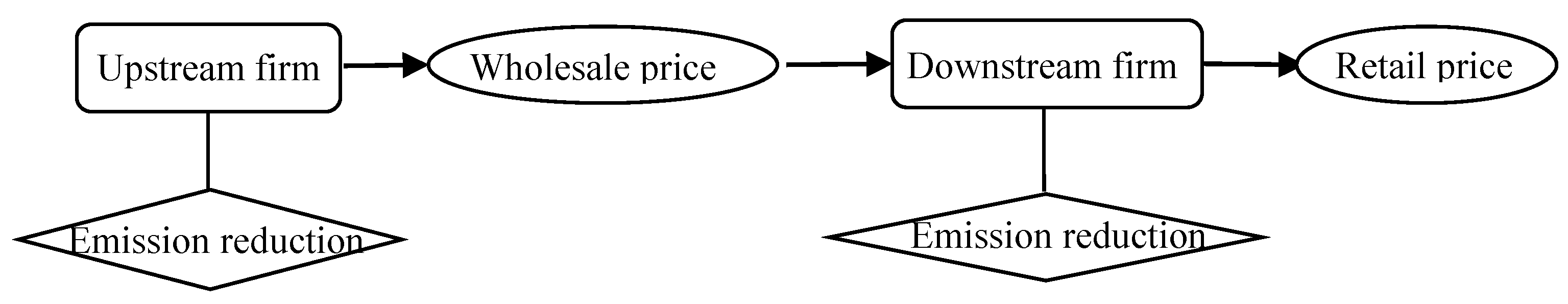
This paper considers a simple supply chain, which consists of an upstream firm and a downstream firm (the subscript $U$ and $D$ in this paper represent variables related to upstream and downstream firms, respectively). The upstream firm produces semi-finished products and sells them to the downstream firm, who produces finished products and sells them in the market. The two firms agree on a wholesale procurement contract. The upstream firm decides the wholesale price, while the downstream firm decides the retail price. The goal of each firm is to maximize profits in the supply chain. Both firms pursue carbon emission reductions due to carbon costs, and carry out their own strategies as well. The operations of the supply chain are demonstrated in Figure 1.

The government allocates a certain free emission allowance to firms in the supply chain. According to the actual implementation of current global low-carbon management policies, this paper considers two main schemes of allocating free emission allowance: by emission intensity and by emission capacity. In the allocation scheme by emission intensity, if the emission level per product of firm $i$ is $e_i$, the output is $q$ and the allocated free emission allowance per product is ${\sigma }_i$, then this firm needs to purchase emission allowance for the quantity of $(e_i-{\sigma }_i)q$ in the carbon market to meet its production requirements. Free allowance allocation based on emission intensity is widely used in many countries or regions running carbon markets, such as California (U.S.), Alberta (CAN), New Zealand, China, and so forth. On the other hand, in the case of allocation scheme by emission capacity, if the total free emission allowance allocated for a firm is $E_i$, the firm needs to purchase emission allowance by eq-E_i. The free allowance is distributed according to historical capacity. This scheme is more convenient to implement, since it does not need to adjust the free allowance by actual production quantity. It has been mainly applied in the European Union carbon trading market [23]. In some extreme cases, if the emissions are lower than the free emission allowance, then the firms may sell the emission permits in the market.

The product’s market demand function is expressed by:

$$p=a-q,$$

(1)

in which the constant $a$ represents market scale. The price of carbon emission permits $p_e$ is given exogenously. To make the solutions feasible, in this paper we assume that the parameters satisfy the condition $a-(c_U+c_D)-p_e(e_U+e_D)>0$, in which $c_U$ and $c_D$ are the production costs for the upstream firm and the downstream firm, respectively. This assumption ensures that the market has enough room of margin to reduce carbon emissions. If the firm determines the emission reduction rate $\lambda$, the emission level per product is reduced from $e$ to $(1-\lambda )e$, incurring an emission abatement cost $k{\lambda }^2/2$. The emission abatement cost $k{\lambda }^2/2$ is an increasing convex function of the emission reduction rate, i.e., the marginal abatement cost increases while the emission decreases. As the emission level drops, further emission reduction becomes more and more difficult. This assumption is consistent with Chen [24], Amacher et al. [25]. The parameter $k$ represents the difficulty of emission reduction. According to the current situation of emission reduction practice, the value of $k$ is relatively high in this study, which represents a considerable cost of emission abatement. This assumption also ensures that there is an internal solution of our models, i.e., the optimal reduction rate $\lambda$ is in the range of [0, 1].

In this paper, we only consider the emission abatement cost as a fixed cost, which is suitable for the following cases: (1) when firms adopt emission abatement technologies such as carbon capture and storage, they do not involve the adjustment of their original production technology and production process. Therefore, it does not affect the variable cost of firms. This emission abatement cost is a fixed cost, which is mainly embodied in the construction of carbon capture and storage devices. (2) When a firm reduces emissions by optimizing the energy consumption of fixed assets such as factory facilities, the variable cost of the products is not affected. (3) When firms improve operations of administrative activities to reduce carbon emissions in aspects such as location, travel, service and so on, the variable production cost does not change. Gurnani et al. and Kaya et al. also used similar assumptions of fixed cost [26,27].

Besides the government stimulation policy such as free emission allowance, firms in the supply chain also take actions to collaborate in reducing carbon emissions. For example, Wal-Mart contributes to share the emission reduction cost of its suppliers proactively. By redistributing emission abatement cost along the supply chain through cost-sharing contracts, the carbon emission can be further reduced. Here, we consider the simplest abatement cost reallocation scheme. Let the upstream firm’s share of the total emission abatement cost be $t$, then the share of the downstream firm is $1-t$. The total emission reduction costs of upstream and downstream firms are ${\displaystyle \sum _{i=U,D}\frac{k{\lambda }_i^2}{2}}$. As a result, the upstream firm pays a cost of $t{\displaystyle \sum _{i=U,D}\frac{k{\lambda }_i^2}{2}}$ and the downstream firm bears a cost of $(1-t){\displaystyle \sum _{i=U,D}\frac{k{\lambda }_i^2}{2}}$.

The sequence of events is as follows. The government first announces the free emission allowance for each firm, ${\sigma }_i$ or $E_i$. If the two firms in the supply chain decide to share the emission abatement cost, then the proportion $t$ is set mutually. Given these important parameters, the two firms then decide their respective emission reduction rate ${\lambda }_U$ and ${\lambda }_D$ at the same time. These decisions could be realized by means such as establishing carbon capture and storage equipment, which may take considerable time, and is thus suitable to be modelled by a simultaneous-move game. After that, the emission reduction rate is observed by both firms and the government. Next, the upstream firm makes a decision on the wholesale price $w_0$. The downstream firm makes a decision on the retail price $p$ after observing the wholesale price. The firms’ pricing decisions can be modelled by a Stackelberg game. The parameters and decision variables are summarized in

Table 1. Parameters and Decision Variables.

Symbols	Descriptions
$e_i$	the emission level per product of firm $i$
${\sigma }_i$	the allocated free emission allowance per product of firm $i$
$E_i$	the total free emission allowance allocated for firm $i$
$k$	the difficulty of emission reduction
$p_e$	the price of carbon emission trading
$a$	market scale, constant
$c_i$	the unit production cost for firm $i$
$t$	the emission abatement cost sharing coefficient
${\lambda }_i$	the emission reduction rate for firm $i$, decision variable
$p$	the retail price for the downstream firm, decision variable
$q$	the production quantity, indirectly determined by the price $p$
$w_0$	the wholesale price of the upstream firm, decision variable

.

3. The Models and Solutions

There are four scenarios based on the combination of two different schemes of free emission allowance allocation and whether firms share emission abatement cost or not. This section will set up a theoretical model and optimize the solutions for each scenario.

3.1. Free Allowance Allocation by Emission intensity without Abatement Cost Sharing (Model 1)

According to the backward derivation rule, we first solve the optimal retail price $p^{\ast }$ for the downstream firm given the emission reduction rate ${\lambda }_U$, ${\lambda }_D$ and the wholesale price $w_0$. The downstream firm’s optimization problem is formulated as:

$$\underset{p}{Max{\pi }_{1D}=}\left(p-w_0-c_D-p_e((1-{\lambda }_D)e_D-{\sigma }_D)\right)(a-p)-\frac{1}{2}k{\lambda }_D^2.$$

(2)

From the first order derivative, we get the expression of the optimal retail price $p^{\ast }$, then introduce it into the upstream firm’s profit function, and determine the optimal wholesale price $w_0$. The upstream firm’s wholesale pricing decision is formulated as:

$$\underset{w_0}{Max{\pi }_{1U}=}\left(w_0-c_U-p_e((1-{\lambda }_U)e_U-{\sigma }_U)\right)(a-p^{\ast })-\frac{1}{2}k{\lambda }_U^2.$$

(3)

After obtaining the optimal wholesale price $w_0^{\ast }$, we introduce it into upstream and downstream firms’ profit functions, respectively. From the first order derivative with respect to the emission reduction rate ${\lambda }_U$, ${\lambda }_D$, we can get the optimal emission reduction rate decisions:

$$\begin{gathered} {\lambda }_{1U}=\frac{{2e}_U{p}_{e}A}{8k-p_e^2(e_D^2+2e_U^2)}, \\ {\lambda }_{1D}=\frac{e_D{p}_{e}A}{8k-p_e^2(e_D^2+2e_U^2)} \end{gathered}$$

(4)

where $A\equiv a-(c_U+c_D)-p_e(e_U+e_D-{\sigma }_U-{\sigma }_D)$ for simplification of expressions.

We derive the upstream and downstream firms’ profit and total profit of supply chain by introducing the optimal emission reduction rate ${\lambda }_{1U}$ and ${\lambda }_{1D}$ into the upstream and downstream firms’ profit functions, respectively:

$$\begin{gathered} {\mathsf{\Pi }}_{1U}=\frac{2k(4k-p_e^2{e}_U^2)A^2}{{(8k-p_e^2(e_D^2+2e_U^2))}^2}, \\ {\mathsf{\Pi }}_{1D}=\frac{k(8k-p_e^2{e}_D^2)A^2}{2{(8k-p_e^2(e_D^2+2e_U^2))}^2}, \end{gathered}$$

(5)

$${\mathsf{\Pi }}_{1T}=\frac{k(24k-p_e^2(e_D^2+4e_U^2))A^2}{2{(8k-p_e^2(e_D^2+2e_U^2))}^2}.$$

(6)

The carbon emission ($C_i$) of the supply chain firm $i$ can be formulated as $C_i=(1-{\lambda }_i)e_{i}q$, thus the total carbon emission of the supply chain can be calculated as $C=[(1-{\lambda }_U)e_U+(1-{\lambda }_D)e_D]q$, which is:

$$C_{1T}=\frac{2kA(8(e_U+e_D)k-p_e(2e_U^2+e_D^2)(p_e{e}_U+p_e{e}_D+A))}{{(8k-p_e^2(e_D^2+2e_U^2))}^2}.$$

(7)

We can also use the average emission $e=(1-{\lambda }_U)e_U+(1-{\lambda }_D)e_D$ to compare and analyze the emission efficiency of the supply chain, which is:

$$e_1=\frac{8(e_U+e_D)k-p_e(2e_U^2+e_D^2)(p_e{e}_U+p_e{e}_D+A)}{8k-p_e^2(e_D^2+2e_U^2)}.$$

(8)

3.2. Free Allowance Allocation by Emission Capacity without Abatement Cost Sharing (Model 2)

Similarly, we can solve this model by the backward derivation rule. The downstream firm’s pricing decision can be expressed as:

$$\underset{p}{Max{\pi }_{2D}=}\left(p-w_0-c_D-e_D{p}_e(1-{\lambda }_D)\right)\left(a-p\right)-\frac{1}{2}k{\lambda }_D^2+E_D{p}_e.$$

(9)

From the first order derivative, we get the expression of the optimal retail price $p^{\ast }$, introduce it into the upstream firm’s profit function and determine optimal wholesale price $w_0$. The upstream firm’s profit is formulated as:

$$\underset{w_0}{Max{\pi }_{2U}=}\left(w_0-c_U-p_e{e}_U(1-{\lambda }_U)\right)\left(a-p^{\ast }\right)-\frac{1}{2}k{\lambda }_U^2+E_U{p}_e.$$

(10)

After obtaining the optimal wholesale price $w_0^{\ast }$, from the first order derivative with respect to emission reduction rate ${\lambda }_U$, ${\lambda }_D$, we can derive the optimal emission reduction rate decisions:

$$\begin{gathered} {\lambda }_{2U}=\frac{{2e}_U{p}_e(A-p_e{\sigma }_U-p_e{\sigma }_D)}{8k-p_e^2(e_D^2+2e_U^2)}, \\ {\lambda }_{2D}=\frac{e_D{p}_e(A-p_e{\sigma }_U-p_e{\sigma }_D)}{8k-p_e^2(e_D^2+2e_U^2)}. \end{gathered}$$

(11)

Similarly, by introducing the optimal emission reduction rate ${\lambda }_{2U}$ and ${\lambda }_{2D}$ into the upstream and downstream firms’ profit functions, respectively, we can get upstream and downstream firms’ profit and total profit of the supply chain:

$$\begin{gathered} {\mathsf{\Pi }}_{2U}=E_U{p}_e+\frac{2k(4k-p_e^2{e}_U^2){(A-p_e{\sigma }_U-p_e{\sigma }_D)}^2}{{(8k-p_e^2(e_D^2+2e_U^2))}^2}, \\ {\mathsf{\Pi }}_{2D}=E_D{p}_e+\frac{k(8k-p_e^2{e}_D^2){(A-p_e{\sigma }_U-p_e{\sigma }_D)}^2}{2{(8k-p_e^2(e_D^2+2e_U^2))}^2}, \end{gathered}$$

(12)

$${\mathsf{\Pi }}_{2T}=(E_U+E_D)p_e+\frac{k(24k-p_e^2(e_D^2+4e_U^2)){(A-p_e{\sigma }_U-p_e{\sigma }_D)}^2}{2{(8k-p_e^2(e_D^2+2e_U^2))}^2}.$$

(13)

According to the formula of total carbon emission and average carbon emission, we get the following results for Model 2:

$$C_{2T}=\frac{2k(A-p_e{\sigma }_U-p_e{\sigma }_D)(8(e_U+e_D)k-p_e(2e_U^2+e_D^2)(a-c_D-c_U))}{{(8k-p_e^2(e_D^2+2e_U^2))}^2},$$

(14)

$$e_2=\frac{8(e_U+e_D)k-p_e(2e_U^2+e_D^2)(a-c_D-c_U)}{8k-p_e^2(e_D^2+2e_U^2)}.$$

(15)

3.3. Free Allowance Allocation by Emission Intensity with Abatement Cost Sharing (Model 3)

Based on Model 1, after introducing the abatement cost sharing contract, the upstream and downstream firm’s decision problem can be respectively formulated as:

$$\underset{p}{Max} {\pi }_{3D}=\left(p-w-c_D-p_e((1-{\lambda }_D)e_D-{\sigma }_D)\right)(a-p)-\frac{1}{2}(1-t)k({\lambda }_U^2+{\lambda }_D^2),$$

(16)

$$\underset{w_0}{Max{\pi }_{3U}=}\left(w-c_U-p_e((1-{\lambda }_U)e_U-{\sigma }_U)\right)(a-p^{\ast })-\frac{1}{2}tk({\lambda }_U^2+{\lambda }_D^2).$$

(17)

Through backward derivation rule, we can get the expressions of the optimal retail price $p^{\ast }$ and then the optimal wholesale price $w_0^{\ast }$, and introduce them into upstream and downstream firms’ profit functions. According to the first order conditions of emission reduction rate ${\lambda }_U$, ${\lambda }_D$,we can get the optimal emission reduction rate decisions:

$$\begin{gathered} {\lambda }_{3U}=\frac{2(1-t{)e}_U{p}_{e}A}{8kt(1-t)-p_e^2(t{e}_D^2+2(1-t)e_U^2)}, \\ {\lambda }_{3D}=\frac{t{e}_D{p}_{e}A}{8kt(1-t)-p_e^2(t{e}_D^2+2(1-t)e_U^2)}. \end{gathered}$$

(18)

To make the firms stay in this supply chain, the cost-sharing proportion cannot be too high or too low. Otherwise, a single firm bearing too much emission abatement cost may not be profitable. The feasible region of ${\lambda }_U$ is calculated in Section 4. Similarly, by introducing the optimal emission reduction rate ${\lambda }_{3U}$ and ${\lambda }_{3D}$ into the upstream and downstream firms’ profit functions respectively, we can get the upstream and downstream firms’ expected profit and the total profit of supply chain:

$$\begin{gathered} {\mathsf{\Pi }}_{3U}=\frac{kt(16kt{(1-t)}^2-p_e^2(t^2{e}_D^2+4{(1-t)}^2{e}_U^2)A^2}{2{(8kt(1-t)-p_e^2(t{e}_D^2+2(1-t)e_U^2))}^2}, \\ {\mathsf{\Pi }}_{3D}=\frac{k(1-t)(8k{t}^2(1-t)-p_e^2(t^2{e}_D^2+4{(1-t)}^2{e}_U^2))A^2}{2{(8kt(1-t)-p_e^2(t{e}_D^2+2(1-t)e_U^2))}^2}, \end{gathered}$$

(19)

$${\mathsf{\Pi }}_{3T}=\frac{k(24k{t}^2{(1-t)}^2-p_e^2(t^2{e}_D^2+4{(1-t)}^2{e}_U^2))A^2}{2{(8kt(1-t)-p_e^2(t{e}_D^2+2(1-t)e_U^2))}^2}.$$

(20)

According to the calculation formula of total carbon emission and average carbon emission, we get the following results for Model 3:

$$C_{3T}=\frac{2kt(1-t)A((e_U+e_D)(8kt(1-t)-p_e^2(t{e}_D^2+2(1-t)e_U^2))-A{p}_e(t{e}_D^2+2(1-t)e_U^2))}{{(8kt(1-t)-p_e^2(t{e}_D^2+2(1-t)e_U^2))}^2},$$

(21)

$$e_3=e_U+e_D-\frac{p_e(2(1-t)e_U^2+t{e}_D^2)A}{8kt(1-t)-p_e^2(t{e}_D^2+2(1-t)e_U^2)}.$$

(22)

3.4. Free Allowance Allocation by Emission Capacity with Abatement Cost Sharing (Model 4)

Based on Model 2, after introducing the abatement cost sharing contract, the upstream and downstream firm’s decision problem can be respectively formulated as:

$$\underset{p}{Max{\pi }_{4D}=}\left(p-w-c_D-e_D{p}_e(1-{\lambda }_D)\right)(a-p)+E_D{p}_e-\frac{1}{2}(1-t)k({\lambda }_U^2+{\lambda }_D^2),$$

(23)

$$\underset{w}{Max} {\pi }_{4U}=\left(w-c_U-e_U{p}_e(1-{\lambda }_U)\right)(a-p^{\ast })+E_U{p}_e-\frac{1}{2}tk({\lambda }_U^2+{\lambda }_D^2).$$

(24)

By steps similar to Model 3, we derive the optimal emission reduction rate decision:

$$\begin{gathered} {\lambda }_{4U}=\frac{2(1-t)e_U{p}_e(A-p_e{\sigma }_U-p_e{\sigma }_D)}{8kt(1-t)-p_e^2(t{e}_D^2+2(1-t)e_U^2)}, \\ {\lambda }_{4D}=\frac{t{e}_D{p}_e(A-p_e{\sigma }_U-p_e{\sigma }_D)}{8kt(1-t)-p_e^2(t{e}_D^2+2(1-t)e_U^2)}. \end{gathered}$$

(25)

On introducing the optimal emission reduction rate ${\lambda }_{4U}$ and ${\lambda }_{4D}$ into upstream and downstream firms’ profit functions, respectively, the upstream and downstream firms’ profit and the total profit of supply chain are:

$$\begin{gathered} {\mathsf{\Pi }}_{4U}=E_U{p}_e+\frac{kt(16kt{(1-t)}^2-p_e^2(t^2{e}_D^2+4{(1-t)}^2{e}_U^2)){(A-p_e{\sigma }_U-p_e{\sigma }_D)}^2}{2{(8kt(1-t)-p_e^2(t{e}_D^2+2(1-t)e_U^2))}^2}, \\ {\mathsf{\Pi }}_{4D}=E_D{p}_e+\frac{k(1-t)(8k{t}^2(1-t)-p_e^2(t^2{e}_D^2+4{(1-t)}^2{e}_U^2)){(A-p_e{\sigma }_U-p_e{\sigma }_D)}^2}{2{(8kt(1-t)-p_e^2(t{e}_D^2+2(1-t)e_U^2))}^2}, \end{gathered}$$

(26)

$${\mathsf{\Pi }}_{4T}=(E_U+E_D)p_e+\frac{k(24k{t}^2{(1-t)}^2-p_e^2(t^2{e}_D^2+4{(1-t)}^2{e}_U^2)){(A-p_e{\sigma }_U-p_e{\sigma }_D)}^2}{2(2(1-t)e_U^2{p}_e^2+{(t^2(e_D^2{p}_e^2-8k(1-t)))}^2}.$$

(27)

The total carbon emission and average carbon emission of the supply chain can be respectively formulated as:

$$C_{4T}=\frac{2kt(1-t)(A-p_e{\sigma }_U-p_e{\sigma }_D)((e_U+e_D)(8kt(1-t)-p_e^2(t{e}_D^2+2(1-t)e_U^2))-(A-p_e{\sigma }_U-p_e{\sigma }_D)p_e(t{e}_D^2+2(1-t)e_U^2))}{{(8kt(1-t)-p_e^2(t{e}_D^2+2(1-t)e_U^2))}^2},$$

(28)

$$e_4=e_U+e_D-\frac{p_e(2(1-t)e_U^2+t{e}_D^2)(A-p_e{\sigma }_U-p_e{\sigma }_D)}{8kt(1-t)-p_e^2(t{e}_D^2+2(1-t)e_U^2)}.$$

(29)

4. Analysis and Discussion

In this section, we analyze the results of the theoretical models in Section 3 and discuss their managerial implications.

Proposition 1.

In the case that firms do not share emission abatement costs, when $2e_U>e_D$, emission reduction rate of the upstream firm is higher than that of the downstream firm; otherwise, emission reduction rate of the downstream firm is higher than that of the upstream firm. In the case that firms share the emission abatement cost, when $2(1-t)e_U>t{e}_D$, emission reduction rate of the upstream firm is higher than that of the downstream firm; otherwise, emission reduction rate of the downstream firm is higher than that of the upstream firm.

Proposition 1 can be easily verified by directly comparing Formulas (4) and (9), and Formulas (18) and (25). The comparison is in the weak sense that equal solutions are not explicitly discussed.

In the special case that the upstream firm and the downstream firm are generating equal emissions, i.e., $e_U=e_D$, we can derive from Proposition 1 that the upstream will implement a higher emission reduction rate when emission abatement cost is not shared. If the two firms share the emission abatement cost, the emission reduction rate of the upstream firm is higher than that of the downstream firm when $t<2/3$.

In summary, the upstream firm has a stronger tendency to set a higher emission reduction rate in the supply chain. Even if the upstream firm has a low carbon emission intensity, as long as it is higher than half of the carbon emission intensity of the downstream firm, the former will still set a higher emission reduction rate. Supply chain structure puts more pressure on the upstream firm to reduce emission, thus weakening the relative motivation of the downstream firm in reducing emissions.

Proposition 2.

The optimal emission reduction rate monotonously decreases with the difficulty of reducing emissions.

Proof. 

To explore the relationship between emission reduction difficulty $k$ and emission reduction rate, we take derivative of (4) with respect to $k$:

$$\frac{\partial {\lambda }_{1U}}{\partial k}=-\frac{16e_U{p}_{e}A}{{(8k-p_e^2(e_D^2+2e_U^2))}^2},$$

(30)

$$\frac{\partial {\lambda }_{1D}}{\partial k}=-\frac{8e_D{p}_{e}A}{{(8k-p_e^2(e_D^2+2e_U^2))}^2}.$$

(31)

${(8k-p_e^2(e_U^2+e_D^2))}^2>0$, $16e_U{p}_e>0$ and $8e_D{p}_e>0$ is always true. Moreover, since A > 0 by assumption, there is a negative relationship between emission reduction rate and difficulty of emission reduction $k$.  ☐

The result of Proposition 2 is consistent with intuition. The more difficult reducing emission is, the lower will be the emission reduction rate set by firms. If a government seeks to promote broad emission reduction, it is fundamental that they make policies to reduce the difficulty of emission reduction.

Proposition 3.

The total carbon emission with abatement cost sharing is lower than that without. When firms in a supply chain share emission abatement costs, the total carbon emission first decreases and then increases in a proportion of the upstream firm’s cost share t.

Proof. 

We first optimize the total carbon emission over $t$ in model 3. Let $\frac{\partial C_{3T}}{\partial t}=0$; we can then get $t^{\ast }$ and find $t^{\ast }\ne \frac{{\lambda }_U}{{\lambda }_U+{\lambda }_D}$. At $t=\frac{{\lambda }_U}{{\lambda }_U+{\lambda }_D}$, Model 1 is equivalent to Model 3. Therefore, the total carbon emission in Model 3 is greater than that of Model 1. Introducing an emission abatement cost sharing contract into the supply chain induces more emission reduction of firms. We can further verify that when $t\in (\frac{8k-e_D^2{p}_e^2-2e_U^2{p}_e^2-\sqrt{64k{e}_U^2{p}_e^2+{(-8k+e_D^2{p}_e^2+2e_U^2{p}_e^2)}^2}}{16k},t^{\ast })$, the total carbon emission is negatively related to the sharing proportion of upstream firm $t$; when $t\in (t^{\ast },\frac{8k-e_D^2{p}_e^2-2e_U^2{p}_e^2+\sqrt{64k{e}_U^2{p}_e^2+{(-8k+e_D^2{p}_e^2+2e_U^2{p}_e^2)}^2}}{16k})$, the total carbon emissions is positively related to $t$.  ☐

Proposition 3 reflects the effectiveness of sharing the emission abatement cost in reducing the total carbon emissions. When the sharing proportion is appropriately designed, the supply chain’s total carbon emission can be further decreased. As the sharing proportion of upstream firm $t$ increases, the total carbon emission of the supply chain first decreases, and then increases. There exists an optimal sharing proportion, which minimizes total carbon emission.

Proposition 4.

When firms in a supply chain share the emission abatement costs, the firms’ optimal emission reduction rate first decreases and then increases in the upstream firm’s sharing proportion t.

Proof. 

In order to explore the relationship between $t$ and ${\lambda }_i$, the first order derivative of formula (18) can be obtained as:

$$\begin{gathered} \frac{\partial {\lambda }_{3U}}{\partial t}=\frac{2e_U{p}_e(e_D^2{p}_e^2-8k{(1-t)}^2)A}{{(8kt(1-t)-p_e^2(t{e}_D^2+2(1-t)e_U^2))}^2}, \\ \frac{\partial {\lambda }_{3D}}{\partial t}=\frac{2e_D{p}_e(e_U^2{p}_e^2-4k{t}^2)A}{{(8kt(1-t)-p_e^2(t{e}_D^2+2(1-t)e_U^2))}^2}. \end{gathered}$$

(32)

Because ${(8kt(1-t)-p_e^2(t{e}_D^2+2(1-t)e_U^2))}^2>0$, $2e_U{p}_e>0$, $2e_D{p}_e>0$, and $A=a-(c_U+c_D)-p_e(e_U+e_D-{\sigma }_U-{\sigma }_D)>0$ are true, and both $e_D^2{p}_e^2-8k{(1-t)}^2$ and $e_U^2{p}_e^2-4k{t}^2$ are dependent of $t$ and their signs are indeterminate, we need to judge the range of this two formula.

For the upstream firm, since ${\lambda }_i\in (0,1)$ is true, we can get $t\in (\frac{8k-e_D^2{p}_e^2+2e_U^2{p}_e^2-\sqrt{-64k{e}_U^2{p}_e^2+{(8k-e_D^2{p}_e^2+2e_U^2{p}_e^2)}^2}}{16k},\frac{8k-e_D^2{p}_e^2+2e_U^2{p}_e^2+\sqrt{-64k{e}_U^2{p}_e^2+{(8k-e_D^2{p}_e^2+2e_U^2{p}_e^2)}^2}}{16k})$. If $t\in (\frac{8k-e_D^2{p}_e^2+2e_U^2{p}_e^2-\sqrt{-64k{e}_U^2{p}_e^2+{(8k-e_D^2{p}_e^2+2e_U^2{p}_e^2)}^2}}{16k},1-\frac{e_D{p}_e}{2\sqrt{2k}})$, we have $\frac{\partial {\lambda }_{3_U}}{\partial t}<0$, which means emission reduction rate is negatively related to the sharing proportion of emission abatement cost for smaller $t$; if $t\in (1-\frac{e_D{p}_e}{2\sqrt{2k}},\frac{8k-e_D^2{p}_e^2+2e_U^2{p}_e^2+\sqrt{-64k{e}_U^2{p}_e^2+{(8k-e_D^2{p}_e^2+2e_U^2{p}_e^2)}^2}}{16k})$, we have $\frac{\partial {\lambda }_{3_U}}{\partial t}>0$, which means emission reduction rate is positively related to the sharing proportion of emission abatement cost for larger $t$.

For the downstream firm, we can similarly calculate that when $t\in (\frac{8k-e_D^2{p}_e^2-2e_U^2{p}_e^2-\sqrt{64k{e}_U^2{p}_e^2+{(-8k+e_D^2{p}_e^2+2e_U^2{p}_e^2)}^2}}{16k},\frac{e_U{p}_e}{2\sqrt{k}})$, the downstream firm’s emission reduction rate is negatively related to upstream firm’s sharing proportion of the total emission abatement costs; when $t\in (\frac{e_U{p}_e}{2\sqrt{k}},\frac{8k-e_D^2{p}_e^2-2e_U^2{p}_e^2+\sqrt{64k{e}_U^2{p}_e^2+{(-8k+e_D^2{p}_e^2+2e_U^2{p}_e^2)}^2}}{16k})$, the downstream firm’s emission reduction rate is negatively related to upstream firm’s sharing proportion of the total emission abatement costs.  ☐

Proposition 4 indicates that as the sharing rate becomes greater, both the upstream firm and the downstream firm’s optimal emission reduction rates first decrease, and then increase. The intuition behind the results may be explained as follows. When the upstream firm’s sharing proportion $t$ is small and increasing, the upstream firm reduces its emission reduction rate because the quantity sold can be increased significantly due to lower margin and the profit is increased; the downstream firm reduces its emission reduction rate because it now bears less emission costs, which require less effort in reducing emissions. When the upstream firm’s sharing proportion $t$ is large and increasing, the upstream firm increases its emission reduction rate because it bears more emission abatement costs, which require more effort in reducing emissions; the downstream firm increases its emission reduction rate because its demand is shrinking as a result of high marginal cost due to the upstream firm’s heavy burden of emission reduction and the downstream firm has a stronger incentive to reduce its marginal cost.

In general, the upstream and downstream firms should balance their margin and sales quantity by choosing emission reduction according to the emission abatement sharing proportion $t$.

Proposition 5.

With free emission allowance allocation scheme by emission intensity, the emission reduction rate of firms is higher than that by emission capacity, regardless of whether emission abatement cost sharing is adopted or not. The difference in emission reduction decisions caused by different free emission allowance allocation schemes first decreases in t and then increases in t.

Proof. 

This proposition can be easily verified by directly comparing Formulas (4) and (11), and Formulas (18) and (25).

In order to explore how cost-sharing proportions impact the difference of emission reduction decisions caused by two free emission allowance allocation schemes, we first calculate the difference between the optimal emission reduction decisions in Model 3 and Model 4 for the upstream firm:

$$\overline{\lambda }={\lambda }_{3U}-{\lambda }_{4U}=\frac{2(1-t)e_U{p}_e^2({\sigma }_U+{\sigma }_D)}{8kt(1-t)-p_e^2(t{e}_D^2+2(1-t)e_U^2)}=\frac{2e_U{p}_e^2({\sigma }_U+{\sigma }_D)}{8kt-\frac{e_D^2{p}_e^2}{1-t}+p_e^2(e_D^2-2e_U^2)}.$$

(33)

Through first order derivative, we can verify that when $t\in (\frac{8k-e_D^2{p}_e^2+2e_U^2{p}_e^2-\sqrt{-64k{e}_U^2{p}_e^2+{(8k-e_D^2{p}_e^2+2e_U^2{p}_e^2)}^2}}{16k},1-\frac{e_D{p}_e}{2\sqrt{2k}})$, $\overline{\lambda }$ is decreasing in $t$; when $t\in (1-\frac{e_D{p}_e}{2\sqrt{2k}},\frac{8k-e_D^2{p}_e^2+2e_U^2{p}_e^2+\sqrt{-64k{e}_U^2{p}_e^2+{(8k-e_D^2{p}_e^2+2e_U^2{p}_e^2)}^2}}{16k})$, $\overline{\lambda }$ is decreasing in $t$. The difference between downstream firms’ decisions in different emission allowance allocation schemes can be analyzed similarly and the result is evident.  ☐

When free emission allowance is allocated by emission capacity, the decision of a firm’s emission reduction rate is mainly influenced by carbon price. The free emission allowance $E$ is not related to production quantity $q$, which does not affect the marginal revenue and marginal cost of the firm, and only affects the final profit of the firm. However, the optimal reduction rate decision depends on the marginal cost. Hence, the free emission allowance $E$ does not affect the emission reduction rate decision. When free emission allowance is allocated by emission intensity, the optimal emission reduction rate is not only influenced by carbon price, but also by the level of free emission allowance. Both of them stimulate firms to reduce emissions and result in a higher emission reduction rate. The total amount of free carbon emission allowance that firms actually have is related to the level of production, so the firms are more motivated to reduce emissions and expand production. According to this conclusion, if governments wants to encourage firms to increase emission reduction rates and reduce total emission levels, the free emission allowance allocation scheme based on emission intensity will have a better effect.

When firms share emission abatement costs, allocating free emission allowance by emission intensity also induces firms to set a higher emission reduction rate. If the upstream firm’s sharing proportion is high or low, the difference in the optimal emission reduction rate is more significant. If the upstream firm’s sharing proportion is moderate, there is less difference in emission reduction rate caused by different free emission allocation schemes. The pattern of changes in the difference in emission reduction rate is similar to that in Proposition 4.

With the emission abatement cost sharing scheme, when the sharing cost is small, the degree of cost sharing is negative to the disparity of two free emission allowance allocation schemes; when the sharing cost is large, the degree of cost sharing is positive to the disparity of two free emission allowance allocation schemes.

Proposition 6.

The relationship between carbon price and emission reduction rate is related to the difficulty of reducing emissions. When the difficulty of emission reduction is low, increasing carbon price is more conducive to improving the emission reduction rate; when the difficulty of emission reduction is high, increasing carbon price will first increase the emission reduction rate and then decrease it.

Proof. 

Since this proposition only considers the relationship between carbon price and emission reduction rate, to simplify and highlight the impact of price changes, we suppose $a=1$, $c_i=0$, and $p_e<\frac{1}{e_U+e_D-{\sigma }_U-{\sigma }_D}$ without loss of generality. Moreover, we know that Model 1 & 2 is a special case of Model 3 & 4 when $t=\frac{{\lambda }_U}{{\lambda }_U+{\lambda }_D}$. Since the sharing proportion $t$ can be regarded as an exogenous parameter, for simplification, we suppose $t=\frac{{\lambda }_U}{{\lambda }_U+{\lambda }_D}$ and take Model 1 and Model 2 as an example for calculation and analysis. Therefore, Formulas (3) and (6) can be simplified as:

$$\begin{gathered} {\lambda }_{1U}^{\prime }=\frac{{2e}_U{p}_e(1-p_e(e_U+e_D-{\sigma }_U-{\sigma }_D))}{8k-p_e^2(e_D^2+2e_U^2)}, \\ {\lambda }_{1D}^{\prime }=\frac{e_D{p}_e(1-p_e(e_U+e_D-{\sigma }_U-{\sigma }_D))}{8k-p_e^2(e_D^2+2e_U^2)}, \end{gathered}$$

(34)

$$\begin{gathered} {\lambda }_{2U}^{\prime }=\frac{{2e}_U{p}_e(1-p_e(e_U+e_D))}{8k-p_e^2(e_D^2+2e_U^2)}, \\ {\lambda }_{2D}^{\prime }=\frac{e_D{p}_e(1-p_e(e_U+e_D))}{8k-p_e^2(e_D^2+2e_U^2)}. \end{gathered}$$

(35)

We use ${\lambda }_i=\frac{e_{i_U}{\lambda }_{i_U}+e_{i_D}{\lambda }_{i_D}}{e_{i_U}+e_{i_D}},i=1,2$ to represent the total emission reduction rate of supply chain in Model $i$, and can be expressed as:

$${\lambda }_1=\frac{{(e}_D^2+2e_U^2)p_e(1-p_e(e_U+e_D-{\sigma }_U-{\sigma }_D))}{(e_U+e_D)(8k-p_e^2(e_D^2+2e_U^2))},$$

(36)

$${\lambda }_2=\frac{(e_D^2+2e_U^2)p_e(1-p_e(e_U+e_D))}{(e_U+e_D)(8k-p_e^2(e_D^2+2e_U^2))}.$$

(37)

According to Formulas (15) and (16), the optimal emission reduction rate with different free emission allowance allocation is affected by carbon price, and varying carbon price will lead to different emission reduction efficiency. Therefore, we take the first order derivative of the optimal emission reduction rate of the supply chain with respect to carbon price under these two different emission abatement cost sharing scenarios. Firstly, we discuss the optimal solutions in Model 1:

$$\frac{\partial {\lambda }_1}{\partial p_e}=\frac{(e_D^2+2e_U^2)((e_D^2+2e_U^2)p_e^2-16k(e_U+e_D-{\sigma }_U-{\sigma }_D)p_e+8k)}{(e_U+e_D){(8k-p_e^2(e_D^2+2e_U^2))}^2}.$$

(38)

If the first order derivative is greater than zero, the optimal emission reduction rate is positively related to carbon price, and vice versa. Since ${(8k-p_e^2(e_U^2+e_D^2))}^2>0$, $e_D^2+2e_U^2>0$ and $e_U+e_D>0$ are true, we only check the range of $(e_U^2+2e_D^2)p_e^2-16k(e_U+e_D-{\sigma }_U-{\sigma }_D)p_e+8k$. Obviously, this formula can be regarded as a quadratic convex function $f_{(p_e)}^1=(e_U^2+2e_D^2)p_e^2-16k(e_U+e_D-{\sigma }_U-{\sigma }_D)p_e+8k$, in which $p_e$ is its independent variable, and the range of $p_e$ is [0, $\frac{1}{e_U+e_D-{\sigma }_U-{\sigma }_D}$). According to the root formula, its discriminant is $\mathsf{\Delta }=256{(e_U+e_D-{\sigma }_U-{\sigma }_D)}^2{k}^2-32(e_D^2+2e_U^2)k$.

If Δ < 0, we have $k<\frac{e_D^2+2e_U^2}{8{(e_U+e_D-{\sigma }_U-{\sigma }_D)}^2}$. The emission reduction difficulty coefficient $k$ is relatively low, hence emission reduction is easy to be realized. $f_{(p_e)}^1$ and the transverse axis have no intersection, which means $f_{(p_e)}^1>0$. As a result, the optimal emission reduction rate is positively related to the carbon price in this case.

If Δ > 0, we have $k>\frac{e_D^2+2e_U^2}{8{(e_U+e_D-{\sigma }_U-{\sigma }_D)}^2}$. The emission reduction difficulty coefficient $k$ is relatively high, so emission reduction is difficult to be realized. $f_{(p_e)}^1$ and the transverse axis have two intersections, $p_e^{-}$ and $p_e^{+}$. They are expressed as:

$$\begin{gathered} p_e^{-}=\frac{8(e_U+e_D-{\sigma }_U-{\sigma }_D)-2\sqrt{-2k(e_D^2+2e_U^2)+16k^2{(e_U+e_D-{\sigma }_U-{\sigma }_D)}^2}}{e_D^2+2e_U^2}, \\ {p}_e^{+}=\frac{8(e_U+e_D-{\sigma }_U-{\sigma }_D)+2\sqrt{-2k(e_D^2+2e_U^2)+16k^2{(e_U+e_D-{\sigma }_U-{\sigma }_D)}^2}}{e_D^2+2e_U^2}. \end{gathered}$$

(39)

Since:

$$\begin{array}{l}{p}_e^{+}-\frac{1}{e_U+e_D-{\sigma }_U-{\sigma }_D}=\frac{1}{e_U+e_D-{\sigma }_U-{\sigma }_D-\frac{\sqrt{-k(e_D^2-2e_U^2)+8k^2{(e_U+e_D-{\sigma }_U-{\sigma }_D)}^2}}{2\sqrt{2}k}}-\frac{1}{e_U+e_D-{\sigma }_U-{\sigma }_D}\\ =\frac{\frac{\sqrt{-k(e_D^2-2e_U^2)+8k^2{(e_U+e_D-{\sigma }_U-{\sigma }_D)}^2}}{2\sqrt{2}k}}{(e_U+e_D-{\sigma }_U-{\sigma }_D-\frac{\sqrt{-k(e_D^2-2e_U^2)+8k^2{(e_U+e_D-{\sigma }_U-{\sigma }_D)}^2}}{2\sqrt{2}k})(e_U+e_D-{\sigma }_U-{\sigma }_D)}\end{array}$$

and we know $e_U+e_D-{\sigma }_U-{\sigma }_D>0$, $\frac{\sqrt{-k(e_D^2-2e_U^2)+8k^2{(e_U+e_D-{\sigma }_U-{\sigma }_D)}^2}}{2\sqrt{2}k}>0$ are true, we just need to determine the range of $e_U+e_D-{\sigma }_U-{\sigma }_D-\frac{\sqrt{-k(e_D^2-2e_U^2)+8k^2{(e_U+e_D-{\sigma }_U-{\sigma }_D)}^2}}{2\sqrt{2}k}$.

For $\frac{\sqrt{-k(e_D^2-2e_U^2)+8k^2{(e_U+e_D-{\sigma }_U-{\sigma }_D)}^2}}{2\sqrt{2}k}=\sqrt{{(e_U+e_D-{\sigma }_U-{\sigma }_D)}^2-\frac{e_D^2-2e_U^2}{8k}}<e_U+e_D-{\sigma }_U-{\sigma }_D$, we can get $e_U+e_D-{\sigma }_U-{\sigma }_D-\frac{\sqrt{-k(e_D^2-2e_U^2)+8k^2{(e_U+e_D-{\sigma }_U-{\sigma }_D)}^2}}{2\sqrt{2}k}>0$, which means $p_e^{+}>\frac{1}{e_U+e_D-{\sigma }_U-{\sigma }_D}$. In the same way, we can get $p_e^{-}<\frac{1}{e_U+e_D-{\sigma }_U-{\sigma }_D}$. Hence, we only need to consider $p_e^{-}$, which is in the feasible range.

When $p_e\in (0,p_e^{-})$, the emission reduction rate is positively related to the carbon price, and emission reduction rate is a concave function of the carbon price. When $p_e\in (p_e^{-},\frac{1}{e_U+e_D-{\sigma }_U-{\sigma }_D})$, emission reduction rate is negatively correlated with the carbon price. When $p_e=p_e^{-}$, there is maximum ${\lambda }_1$.

We then discuss the optimal solutions in Model 2. It is similar to Model 1, regardless of the calculation process or analysis results. Thus, we do not discuss them individually here. When $p_e\in (0,p_e^{-})$, the emission reduction rate is positively correlated with carbon price, and emission reduction rate is a concave function of carbon price. When $p_e\in (p_e^{-},\frac{1}{e_U+e_D})$, the emission reduction rate is negatively correlated with carbon price. When $p_e=p_e^{-}$, there is maximum ${\lambda }_2$.

In general, the relationship between the optimal emission reduction rate and carbon price is similar under different free emission allowance allocation schemes. The key influencing factor is the difficulty of reducing emissions, $k$.

When Δ < 0, which means emission reduction difficulty coefficient $k$ is relatively low, the optimal emission reduction rate is positively related to carbon price. The main reason is that if emission reduction is not difficult, increasing carbon price will motivate firms to increase investments in emission reduction; the optimal emission reduction rate will then be increased accordingly. On the contrary, if carbon price falls, return on investment is not high, and firms will no longer invest a lot of time, energy and funds to reduce emission; emission reduction rate will then fall accordingly. In order to motivate firms to increase investments in emission reduction and enhance their emission reduction rates, a higher carbon price is effective.

When Δ > 0, which means emission reduction difficulty coefficient $k$ is relatively high, as the price of carbon emission increases, the optimal emission reduction rate first increases, and then decreases, and at $p_e=p_e^{-}$, there is maximum emission reduction rate. The intuition is, when the carbon price is low, increasing carbon price will give firms more incentives to reduce the emissions; when the carbon price is high, because $k$ is so large and revenues are shrinking, the supply chain gradually cannot support high rates of emission reduction under the profit pressure; thus, the emission reduction rate declines.

5. Numerical Analysis

To make the results clearer and explore more managerial implications, we carry out numerical analysis through the software Mathematica, version 8.0. The parameters are set as $a=1$, $c_i=0$, $e_U=1.7$, $e_D=1.2$, ${\sigma }_U=2.2$, ${\sigma }_D=0.345$. This combination of parameters is chosen as it can represent the most typical scenarios in our models. The calculations are based on equations we derived in Section 3 and Section 4, and are visualized in the following Figures. Further managerial implications are then presented.

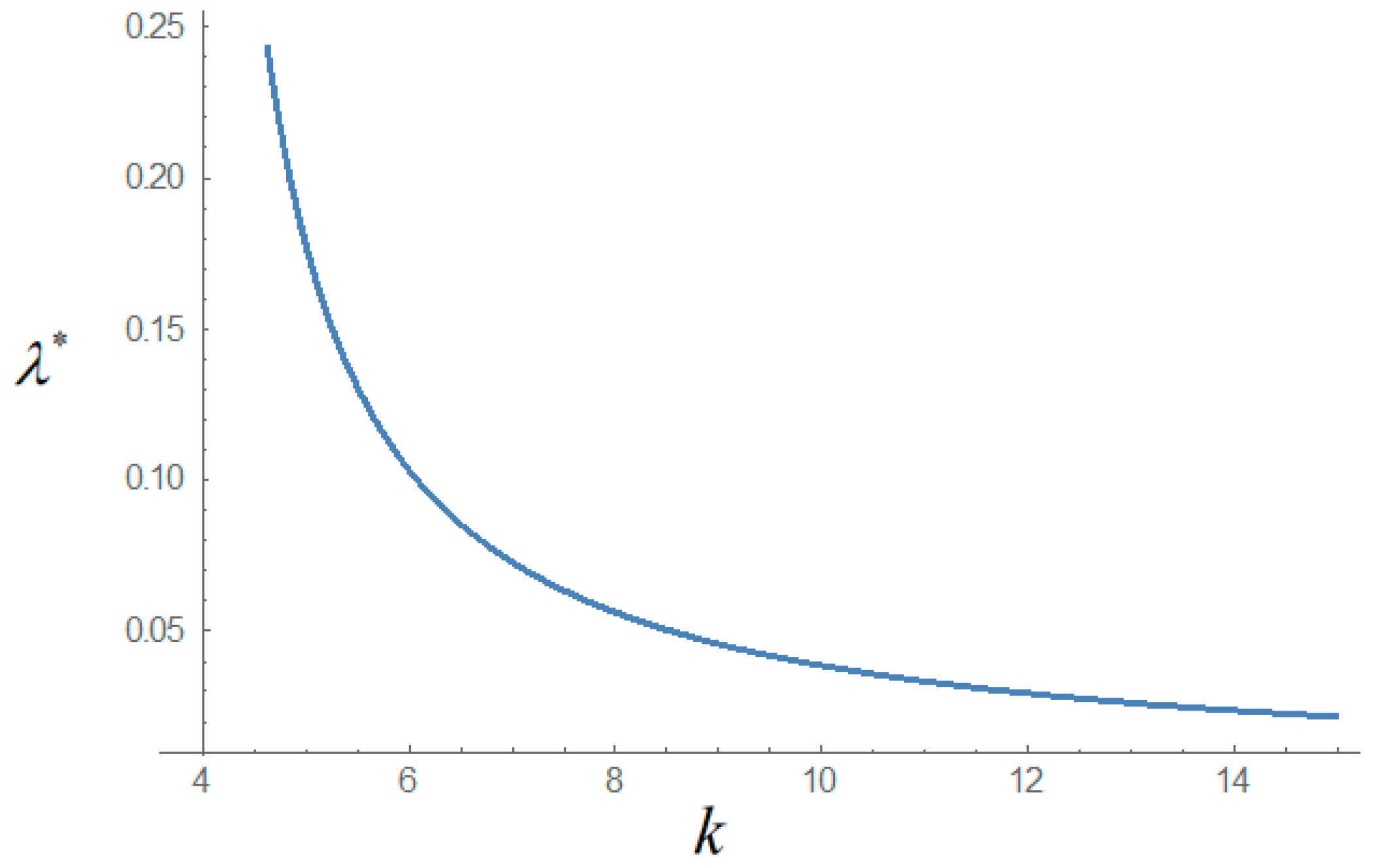
5.1. Relationship between ${\lambda }^{\ast }$ and $k$

Let carbon price be $p_e=2$. The relationship between the difficulty coefficient of reducing carbon emissions and firm’s optimal emission reduction rate is depicted in Figure 2.

From Figure 2, we observe that as reducing emissions becomes more difficult and costly, the firm’s optimal emission reduction rate first decreases very quickly, and then slowly. There exists a turning point in the curve. In industries with a large $k$, a small reduction of $k$ does not lead to significant emission reductions. The government or firms are required to reduce the difficulty of emission reduction beyond that turning point to gain significant emission reduction.

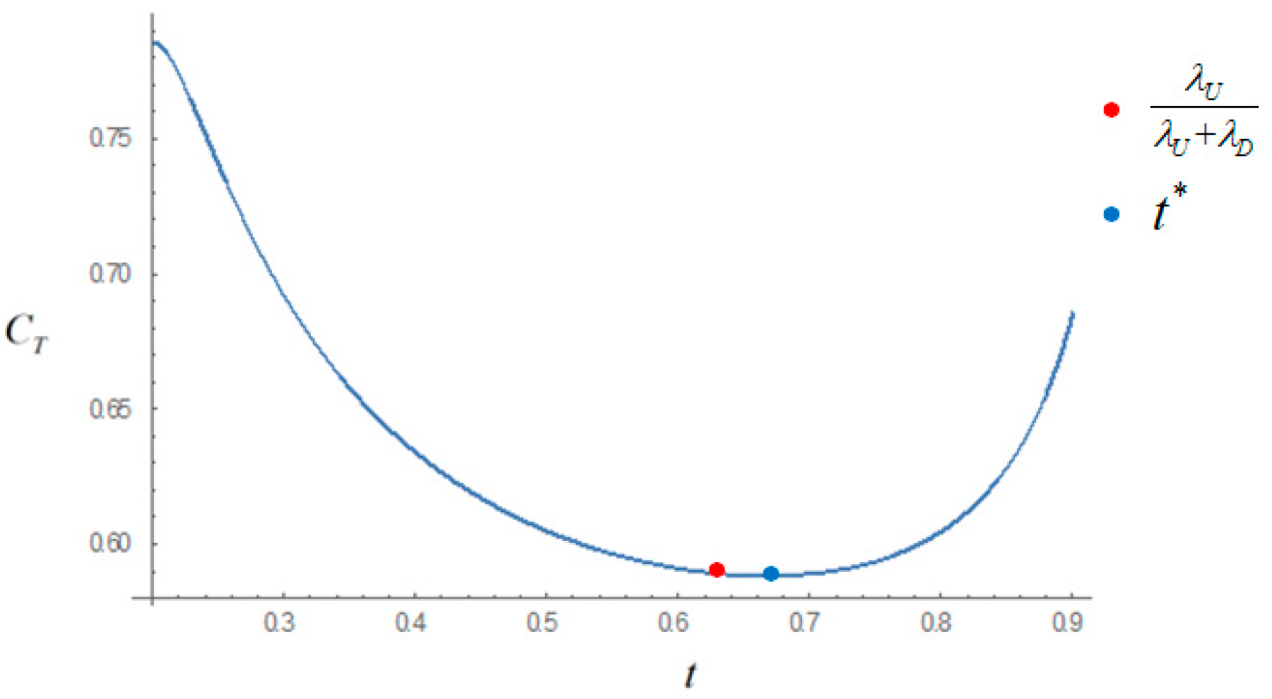
5.2. Relationship between $C_T$ and $t$

We assign $k=6$ and $p_e=1$ in this example to analyze the influence of the sharing proportion of emission abatement cost on the total carbon emission of the supply chain.

From Figure 3, we observe that there is an optimal cost sharing proportion that minimizes the total carbon emission of the supply chain. This optimal sharing proportion is larger than $\frac{{\lambda }_U}{{\lambda }_U+{\lambda }_D}$, which means that the upstream firm should take more share of the supply chain’s emission abatement cost in order to achieve an optimal emission level. As a consequence, the government and supply chain firms should encourage the upstream firm to take more actions in reducing carbon emissions.

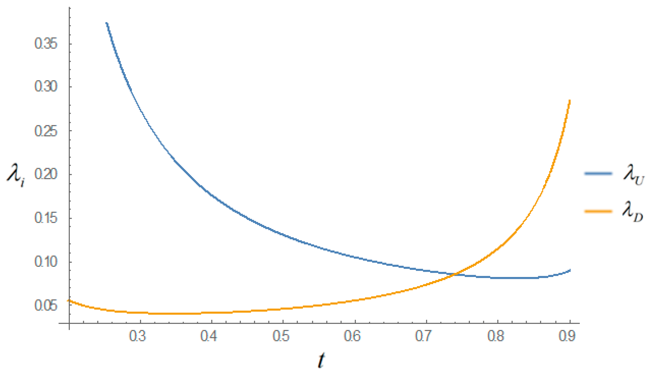
5.3. Relationship between ${\lambda }^{\ast }$ and $t$

Using the same parameters as the previous example, we depict the relationship between the optimal emission reduction rate for the upstream and downstream firms and the cost-sharing proportion $t$ in Figure 4.

Figure 4 shows that the sharing proportion of abatement cost and the optimal emission reduction rate are not in a simple monotonous relationship as concluded in Proposition 5. By combining Figure 3 and Figure 4, we have an interesting observation. At $t^{\ast }$, which minimizes the supply chain’s total carbon emission, both the upstream firm and the downstream firm adopt a relatively low emission reduction rate. Therefore, the supply chain’s emission reduction is achieved by coordinating the two firms in their emission reduction decisions, not by a great effort of a single firm.

5.4. Relationship between ${\lambda }^{\ast }$ and $p_e$

We analyze the influence of carbon price on the emission reduction rate of supply chain through numerical examples. The updated parameters are shown in the caption of the following figures.

The results in Figure 5 and Figure 6 are consistent with the part of low $k$ in Proposition 6. We observe that the optimal emission reduction rate is positively related to carbon price. Firms in the supply chain will choose to reduce emissions by themselves rather than obtain emission permits from the carbon market as carbon price increases. Thus, the optimal emission reduction rate increases moderately with an increase of carbon price at first. After a certain point, as the carbon price increases, the emission reduction rate will increase rapidly. The main reason is that selling emission permits to the market becomes profitable when carbon price is high and reducing emissions is easy. Thus, firms will make large investments on carbon emission reduction and the emission reduction rate will increase sharply.

Therefore, if emission reduction is not difficult, a high carbon price is beneficial to motivate firms to increase investments in emission reduction and thus their emission reduction rates.

The results in Figure 7 and Figure 8 are consistent with Proposition 6 when $k$ is high. There exists an optimal carbon price to maximize emission reduction. When reducing emissions is difficult and costly, simply increasing carbon price does not necessarily lead to a firm’s higher emission reduction rate. If carbon price exceeds a certain critical level, it erodes a firm’s profit. As a result, firms cannot support high emission rates. We can verify that when the emission reduction rate decreases to zero, the profit of each firm is zero, too. Therefore, when emission reduction is difficult, a moderate carbon price is helpful for firms to enhance their emission reduction rate.

6. Conclusions

This study analyzes a supply chain considering different free emission allocation schemes and emission abatement cost sharing, and compares corresponding emission reduction effects. The models introduce emission reduction decision and emission reduction cost into the classical supply chain, analyzing the supply chain performance from the perspective of emission reduction. Based on the optimal solutions of the models, we compare the different characteristics of the upstream and downstream firms in terms of emission reduction decisions. The models are extensions of traditional supply chain models focusing on profit as the main goal, and the results provide managerial insights for firms to reduce carbon emissions in the supply chain scope.

The conclusions drawn from the study have practical instructive significance for improving emission reduction rates and reducing carbon emission in the supply chain. If firms in a supply chain aim to reduce carbon emissions, they should advocate for upstream and downstream firms to establish emission abatement cost sharing schemes; the upstream firms should undertake larger emission reduction costs, and use free emission allowance allocation schemes based on emission intensity. An appropriate sharing proportion of emission abatement cost between upstream firms and downstream firms plays an important role in the corresponding emission reduction decisions. Regardless of which free emission allowance allocation scheme is used or whether abatement cost sharing exists, the upstream firm tends to set a higher emission reduction rate. The government may consider setting rewards for upstream firms. The supply chain’s emission reduction rate is closely related to carbon price. However, the relationship can be significantly affected by the difficulty to reduce emissions. If reducing emissions is extremely difficult or costly, simply increasing the carbon price may not encourage firms to further reduce their carbon emissions. If the government has the ability to intervene in carbon prices, it needs to set a target price on careful evaluation of the difficulty of emission reduction in the supply chain.

This study inevitably has limitations. The employed model only considers the simplest supply chain consisting of two firms, and apparently, there is spacious room for model extension. Future research may further consider the issue of emission reduction control strategies for a more comprehensive supply chain that consists of a number of upstream and downstream firms. Besides, the model implicitly assumes that the information for making emission reduction decisions is complete and symmetric, while the follow-up study may discuss how to effectively encourage the firms in a supply chain to reduce emissions under the condition of asymmetric information. Underpinned by the basis of theoretical analysis, future research can find appropriate empirical evidence to support the theoretical results.

References

- Stern, N. The Economics of Climate Change. Am. Econ. Rev. 2008, 98, 1–37. [Google Scholar] [CrossRef] [Green Version]
- Dales, J.H. Land, Water, and Ownership. Can. J. Econ./Revue Canadienned’ Economique 1968, 29, 256–259. [Google Scholar] [CrossRef]
- Martin, R.; Preux, L.B.; Wagner, U.J. The Impact of a Carbon Tax on Manufacturing: Evidence from Microdata. J. Public Econ. 2014, 117, 1–14. [Google Scholar] [CrossRef] [Green Version]
- Barker, T.; Junankar, S.; Pollitt, H.; Summerton, P. Carbon Leakage from Unilateral Environmental Tax Reforms in Europe, 1995–2005. Energy Policy 2007, 35, 6281–6292. [Google Scholar] [CrossRef]
- Liu, Z.; Davis, S.J.; Feng, K.; Hubacek, K.; Liang, S.; Anadon, L.D.; Chen, B.; Liu, J.; Yan, J.; Guan, D. Targeted Opportunities to Address the Climate-trade Dilemma in China. Nat. Clim. Chang. 2016, 6, 201–206. [Google Scholar] [CrossRef] [Green Version]
- Allevi, E.; Gnudi, A.; Konnov, I.V.; Oggioni, G. Evaluating the effects of environmental regulations on a closed-loop supply chain network: A variational inequality approach. Ann. Oper. Res. 2018, 1, 1–43. [Google Scholar] [CrossRef]
- Hua, G.; Cheng, T.C.E.; Wang, S. Managing Carbon Footprints in Inventory Management. Int. J. Prod. Econ. 2011, 132, 178–185. [Google Scholar] [CrossRef]
- Arıkan, E.; Jammernegg, W. The Single Period Inventory Model Under Dual Sourcing and Product Carbon Footprint Constraint. Int. J. Prod. Econ. 2014, 157, 15–23. [Google Scholar] [CrossRef]
- Yuan, B.; Gu, B.; Guo, J.; Xia, L.; Xu, C. The Optimal Decisions for a Sustainable Supply Chain with Carbon Information Asymmetry under Cap-and-Trade. Sustainability 2018, 10, 1002. [Google Scholar] [CrossRef]
- He, X.; Zhang, J. Supplier Selection Study under the Respective of Low-Carbon Supply Chain: A Hybrid Evaluation Model Based on FA-DEA-AHP. Sustainability 2018, 10, 564. [Google Scholar] [CrossRef]
- D’Aspremont, C.; Jacquemin, A. Cooperative and Noncooperative R&D in Duopoly with Spillovers. Am. Econ. Rev. 1988, 78, 1133–1137. [Google Scholar]
- Kamien, M.; Muller, E.; Zhang, I. Research Joint Ventures and R&D Cartels. Am. Econ. Rev. 1992, 82, 1293–1306. [Google Scholar]
- Guiffrida, A.L.; Nagi, R. Cost Characterizations of Supply Chain Delivery Performance. Prod. Econ. 2006, 102, 22–36. [Google Scholar] [CrossRef]
- Matsui, K. Cost-based Transfer Pricing Under R&D Risk Aversion in an lntegrated Supply Chain. Int. J. Prod. Econ. 2011, 139, 69–79. [Google Scholar] [CrossRef]
- Toptal, A.; Çetinkaya, B. How Supply Chain Coordination Affects the Environment: A Carbon Footprint Perspective. Ann. Oper. Res. 2017, 250, 487–519. [Google Scholar] [CrossRef]
- Soleimani, F.; Khamseh, A.A.; Naderi, B. Optimal Decisions in a Dual-Channel Supply Chain Under Simultaneous Demand and Production Cost Disruptions. Ann. Oper. Res. 2016, 243, 301–321. [Google Scholar] [CrossRef]
- Turki, S.; Didukh, S.; Sauvey, C.; Rezg, N. Optimization and Analysis of a Manufacturing–Remanufacturing–Transport–Warehousing System within a Closed-Loop Supply Chain. Sustainability 2017, 9, 561. [Google Scholar] [CrossRef]
- Turki, S.; Sauvey, C.; Rezg, N. Modelling and optimization of a manufacturing/remanufacturing system with storage facility under carbon cap and trade policy. J. Clean. Prod. 2018, 193, 441–458. [Google Scholar] [CrossRef]
- Caro, F.; Corbett, C.J.; Tan, T.; Zuidwijk, R. Double Counting in Supply Chain Carbon Footprinting. Manuf. Serv. Oper. Manag. 2013, 15, 545–558. [Google Scholar] [CrossRef] [Green Version]
- Du, S.; Ma, F.; Fu, Z. Game-theoretic Analysis for an Emission-Dependent Supply Chain in a ‘Cap-and-Trade’ System. Ann. Oper. Res. 2015, 228, 135–149. [Google Scholar] [CrossRef]
- Roy, A.; Sana, S.S.; Chaudhuri, K. Optimal Pricing of competing retailers under uncertain demand-a two layer supply chain model. Ann. Oper. Res. 2018, 260, 481–500. [Google Scholar] [CrossRef]
- Corbett, C.J.; Decroix, G.A.; Ha, A.Y. Optimal Shared-Savings Contracts in Supply Chains: Linear Contracts and Double Moral Hazard. Eur. J. Oper. Res. 2005, 163, 653–667. [Google Scholar] [CrossRef]
- Hood, C. Reviewing Existing and Proposed Emissions Trading Systems. Int. Energy Agency 2010. IEA Energy Paper No. 2010/13. [Google Scholar]
- Chen, C. Design for the Environment: A Quality-Based Model for Green Product Development. Manag. Sci. 2001, 47, 250–263. [Google Scholar] [CrossRef]
- Amacher, G.S.; Koskela, E.; Ollikainen, M. Environmental quality competition and eco-labeling. J. Environ. Econ. Manag. 2004, 47, 284–306. [Google Scholar] [CrossRef] [Green Version]
- Gurnani, H.; Erkoc, M. Supply Contracts in Manufacturer-Retailer Interactions with Manufacturer-Quality and Retailer Effort-Induced Demand. Nav. Res. Logist. 2008, 55, 200–217. [Google Scholar] [CrossRef]
- Kaya, M.; Özer, Ö. Quality Risk in Outsourcing: Noncontractible Product Quality and Private Quality Cost Information. Nav. Res. Logist. 2009, 56, 669–685. [Google Scholar] [CrossRef]
Figure 1.
The operations of the supply chain.
Figure 2.
Relationship between and (Model 1, upstream firm).
Figure 3.
Relationship between and (Model 3).
Figure 4.
Figure 5.
Relationship between and (Δ < 0, , Model 1).
Figure 6.
Relationship between and (Δ < 0, , Model 2).
Figure 7.
Relationship between and (Δ > 0, , Model 1).
Figure 8.
Relationship between and (Δ > 0, , Model 2)).