Spatially Explicit Soil Compaction Risk Assessment of Arable Soils at Regional Scale: The SaSCiA-Model


1
Department of Geography, Landscape Ecology and Geoinformation Science, Kiel University, Ludewig-Meyn-Str. 14, 24118 Kiel, Germany
2
Department of Geography, Earth Observation and Modelling, Kiel University, Ludewig-Meyn-Str. 14, 24118 Kiel, Germany
*
Author to whom correspondence should be addressed.
Sustainability 2018, 10(5), 1618; https://doi.org/10.3390/su10051618
Submission received: 18 April 2018
/
Revised: 13 May 2018
/
Accepted: 15 May 2018
/
Published: 17 May 2018
(This article belongs to the Special Issue Agriculture, Landscape, Ecosystem Services and Biodiversity: New Challenges for Sustainable Development)
Abstract
:Soil compaction caused by field traffic is one of the main threats to agricultural landscapes. Compacted soils have a reduced hydraulic conductivity, lower plant growth and increased surface runoff resulting in numerous environmental issues such as increased nutrient leaching and flood risk. Mitigating soil compaction, therefore, is a major goal for a sustainable agriculture and environmental protection. To prevent undesirable effects of field traffic, it is essential to know where and when soil compaction may occur. This study developed a model for soil compaction risk assessment of arable soils at regional scale. A combination of (i) soil, weather, crop type and machinery information; (ii) a soil moisture model and (iii) soil compaction models forms the SaSCiA-model (Spatially explicit Soil Compaction risk Assessment). The SaSCiA-model computes daily maps of soil compaction risk and associated area statistics for varying depths at actual field conditions and for entire regions. Applications with open access data in two different study areas in northern Germany demonstrated the model’s applicability. Soil compaction risks strongly varied in space and time throughout the year. SaSCiA allows a detailed spatio-temporal analysis of soil compaction risk at the regional scale, which exceed those of currently available models. Applying SaSCiA may support farmers, stakeholders and consultants in making decision for a more sustainable agriculture.
1. Introduction
Soil compaction represents one of the main threats to soils worldwide [1]; it causes increased surface runoff, soil erosion and nutrient leaching, while infiltration rate, plant growth, root growth and biological activity decrease [2,3,4]. Hence, soil compaction affects soil functionality, agricultural productivity, food security, flood risk and nutrient input to water bodies [5,6,7].
Soil compaction occurs when the exposure to field traffic exceeds soil strength [2]. It is commonly separated into topsoil and subsoil compaction. While primary tillage may reverse topsoil compaction, subsoil compaction persists in the long term [8,9]. Restoring compacted subsoil by e.g., deep loosening is cost and time-consuming; resulting unstable soil conditions prohibit wheeling with heavy machinery after loosening [10]. Preventing soil compaction, in particular subsoil compaction, is therefore the best way to preserve soil functionality.
A first step to prevent soil compaction is the knowledge about where and when soil compaction may occur. A spatial evaluation of soil compaction risk of arable soils is challenging. Highly dynamic natural processes such as the variation in soil moisture strongly influence soil compaction risk [9,11,12]. Moreover, anthropogenic influence by soil management and wheeling activities continuously changes soil properties [13]. Over the last decades, masses and sizes of agricultural machinery increased noticeably resulting in higher loads and stresses imposed on the soils [14]. To minimize undesirable effects of heavy-load field traffic, a reliable estimation of soil compaction risk gains increasing importance. Here, risk means the risk of soil damage (soil compaction) through a certain event such as wheeling activity. The risk is high when the susceptibility to soil compaction of soil (soil properties, wetness) is high and wheeling activities occur (e.g., sowing, fertilizing, harvesting period). The risk is low when wheeling activities are unlikely even if the susceptibility is high (e.g., [11,14]).
Despite its importance, only few approaches exist to estimate soil compaction risk. Most studies focus on the interaction between tire and soil surface, and stress propagation in the soil under single wheels (e.g., [15,16,17,18]). Models developed from these studies such as SOILFlex [19] and Terranimo [20] enable the evaluation of soil compaction risk at single points for individual machines. These models are well suited to support farmers to estimate the potential trafficability of a single point/field.
Studies dealing with soil compaction risk at field, regional or higher scale are rare [21,22,23]. Jones et al. [21] developed a generalized approach to calculate the subsoil compaction risk for Europe. The authors suggested the use of data with higher spatial resolution in combination with pedotransfer functions to improve the prediction of soil compaction risk. Pedotransfer functions calculate soil properties (e.g., field capacity, hydraulic conductivity) based on available soil data (e.g., soil texture, carbon content). SOCOMO, a model developed by van den Akker [22], derives maps of calculated maximum allowable wheel loads. Assuming static soil moisture conditions and static machinery setup, however, limits this approach. Van den Akker and Hoogland [24] applied the approaches from Jones et al. [21] and van den Akker [22] to the Netherlands. Although both models identified the same risk areas, the validation with measured laboratory data was low [24].
Horn and Fleige [15] published a frequently used method to calculate soil compaction risk at different spatial scales. This method is based on the precompression-stress-concept as described in detail by DVWK 234 [25] and Horn and Fleige [15]. It uses pedotransfer functions to calculate the soil compaction risk for two different soil moistures (suction rate of −6 kPa and −30 kPa, respectively, pF 1.8 and 2.5). Horn et al. [23] and Horn and Fleige [26] applied this approach from the farm scale to the supra-regional scales. To estimate the soil compaction risk at the spatial scale, they used constant stress scenarios (e.g., 60 kPa for low and 200 kPa for high stress) for the entire regions. Fritton [27] applied the Horn and Fleige [15] approach for Pennsylvania (USA), D’Or and Destain [28] for Wallonia (Belgium). Following the same approach, Duttmann et al. [29] presented a 3D-model to assess the soil compaction risk caused by silage maize harvest. Although the approach of Horn and Fleige [15] is often used for spatial soil compaction risk assessment, it is controversially discussed (e.g., [30,31]). One criticism addresses the fact that the prediction of soil compaction risk only accounts for two states of soil moistures (pF 1.8 and pF 2.5). Trafficability depends on the current soil water content [9,12]; the Horn and Fleige [15] approach, however, is limited to assess the potential soil compaction risk. It further neglects temporal changes and spatial heterogeneity in soil moisture. Moreover, the aforementioned studies assumed constant soil stresses for the investigated regions, but disregard the real conditions in terms of crop types, soil tillage and machinery setups.
Rücknagel et al. [32] therefore developed a new approach, which enables a soil compaction risk assessment for any soil moisture condition. Using this model, Götze et al. [33] demonstrated the variation of soil compaction risk during the growing season at the farm scale. Their results clearly showed the dynamic changes of load bearing capacity of the soil and, hence, the risk of soil compaction. Hitherto, this approach is limited to single fields where measured soil moisture is available.
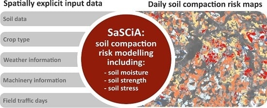
The aim of this study was (1) to develop and (2) to apply a soil compaction model for an assessment of soil compaction risk at the regional scale for dynamic field conditions. To this end, we developed the SaSCiA-model (Spatially explicit Soil Compaction risk Assessment) operating upon readily and freely available data and software. The SaSCiA-model incorporates (i) soil, weather, crop and machinery information; (ii) a soil moisture model (MONICA, [34]) and (iii) soil compaction models [15,32,35]. Considering the dynamic changes of soil properties depending on the present crop types and growing stage, we hypothesize that the SaSCiA-model supports a more realistic estimation of soil compaction risk at regional scale compared to currently available models. The term “regional scale” as it is used in the presented study means a spatial extent of landscape between tens to thousands of square kilometers. To demonstrate the applicability of the model, SaSCiA was applied at two study areas with different soil and weather conditions in northern Germany.
Applying the SaSCiA-model enables the production of daily maps of soil compaction risk, identification of areas exposed to soil compaction and estimation of optimal field traffic days. These regional maps are essential to understand where and to what extent soil compaction may occur. Furthermore, these maps may help to prevent soil compaction by e.g., showing the effects of adapted management strategies.
2. The SaSCiA-Model-Material and Methods
Figure 1 provides a schematic overview of the SaSCiA-model. Input data include weather information, soil data, crop information, machinery setups and field traffic days. Using this input data, the SaSCiA-model generates daily maps of soil compaction risk estimates for entire regions by coupling various models. In detail, it involves spatially explicit
- -
- modelling of soil water content at daily intervals using the MONICA-model [34],
- -
- -
The model is implemented in “R” (version 3.3.1, [38]). Data and models employed are freely available to enable widespread application by interested users. The script including a test dataset is available on request from corresponding author. In case of adaptations or modifications, users can easily replace individual modules or data sets.
2.1. Input Data and Data Preparation
The required input data for the model are weather data, soil data, present crop type, crop information (fertilizer applications; irrigation; dates of sowing, harvest and primary tillage), machinery information and days of field traffic. Soil data and present crop types must be provided as spatially explicit (raster) data. All other input data have to be stored as tables (CSV).
2.1.1. Weather Information
The weather information is necessary to calculate the actual soil moisture with the MONICA-model. The model requires daily values of temperature (average, minimum and maximum), wind speed, precipitation, relative humidity and sun duration (Table A1, Appendix A).
2.1.2. Soil Data
The soil data are used to calculate soil moisture and soil strength. A minimum set of soil parameters includes soil texture class, dry bulk density, gravel content, organic carbon content, soil aggregate structure, air capacity, field capacity, available field capacity and horizon depths. The soil data is required as soil profiles (soil data from soil surface to a depth of 2 m). Additionally, each soil profile must be identifiable by a unique soil identifier (“soil-ID”). The soil profile information has to be stored in a table (Table A2, Appendix A). Moreover, the spatial distribution of all soil profile/soil identifier must be provided as raster data.
2.1.3. Present Crop Types
Knowing the present crop types for the year of soil compaction risk assessment is essential. The cultivated crop type affects the soil moisture of a certain soil and determines the field traffic activities (e.g., times of sowing, fertilizing, spraying, harvesting, used machinery). The crop type information must also be provided as raster data. A reclassification of the crop types by unique crop identifiers (“crop-ID”) converts the raster into a structure readable for the SaSCiA-model. Table A6 (Appendix A) lists the assigned crop-IDs.
2.1.4. Crop Rotation
To consider the effects of previously cultivated crop types on the water balance of the soil, a three-year crop rotation is assumed. The present crop type and the crop types of the preceding two years compose the crop rotation. Intersecting the spatial distribution of crop types from the three consecutive years results in a raster with all possible combinations of crop rotations; a unique identifier (“rotation-ID”) clearly distinguishes all combinations. Figure A1 (Appendix A) demonstrates this principle exemplarily. Joining the “rotation-ID” and “crop-ID”-raster results in a “crop-rotation-ID”-raster, which is used to spatially allocate the crop-information in the SaSCiA-Model.
If the crop type of a previous year is unknown, a representative crop rotation has to be assumed, e.g., winter wheat, winter barley and sugar beet.
In addition to the spatial allocation of the individual crop-rotations, further crop information such as tillage, sowing and harvest dates and tillage depth needs to be added (Table A3, Appendix A).
2.1.5. Fertilizer and Irrigation Information
Information about nitrogen application and irrigation can be included to stimulate plant growth. This information must be stored in individual tables (Table A4, Appendix A). Input parameters include the “crop-rotation-ID”, amount of nitrogen, kind of fertilizer, the application date and incorporation for fertilizer application. For irrigation, the “crop-rotation-ID”, amount of irrigation water and date of irrigation are necessary. Fertilizer and irrigation information is assigned to the crop types based on the “crop-rotation-ID”.
2.1.6. Machinery Information and Field Traffic Days
The machinery used and machinery characteristic are crucial to calculate the mechanical stress imposed on the soil. Therefore, wheel load, tire inflation pressure and field traffic days need to be parameterized for each field. Due to a huge variety of agricultural machinery, the spatial allocation of machinery used on the different fields of a region is mostly unknown.
To enable both, a spatially and a crop type dependent differentiation, the user has to define typical machinery setups used in the study area for each crop type, based on e.g., literature review and manufacturer’s information. In general, the same machinery setup will be applied for each crop type (e.g., maize, sugar beet) within the entire study area.
A similar assumption is required for field traffic activities. The time of field traffic is highly variable at regional scale. To achieve a region-specific approximation, reasonable periods of field traffic activities for each crop type have to be predetermined (if the real dates are unknown). Typical field operations, e.g., primary tillage, sowing and harvest form categories of periods. Each category contains a date for the beginning and ending of potential field traffic activity. The wheel loads and tire inflation pressures are related to each period and crop type. One value for wheel load and tire inflation pressure can be considered per period and crop type. Table A5 (Appendix A) shows an example of the table structure for the machinery and field traffic days.
2.2. Soil Moisture Modelling (MONICA)
Soil compaction risk mainly depends on the soil moisture. Wet soils have a low load bearing capacity and a high susceptibility to soil compaction [39,40]. Increasing desiccation reduces the susceptibility to soil compaction. The actual soil moisture therefore is essential to evaluate field traffic activities on soil functionality. Soil moisture varies strongly, temporally, spatially and with depth. Thus, a continuous update of soil moisture in space and time is necessary to increase the reliability of soil compaction risk assessment.
At the regional scale, soil moisture models may overcome the limited field measurements to provide such an update. A variety of models exist to determine soil moisture; they often are included in crop-growth models (e.g., HYDRUS, DAISY). For the SaSCiA-model, the crop-model MONICA (version 2.0, [34]) was selected. MONICA computes daily soil moisture content at 10 cm depth intervals from top to a depth of 2 m. Several studies demonstrated the usability of the model (e.g., [41,42]). MONICA is applicable to freely available data and transferable to regional scale [41]. Nendel et al. [34] and Nendel and Specka [43] give a detailed description of MONICA.
Soil data, crop type and rotation data, fertilizer data and weather information form the input tables for soil moisture modelling with MONICA in the SaSCiA-model. Matching soil and crop tables results in all possible combinations between soil profiles and crop types. Each combination receives a unique identifier (“soil-crop-rotation-ID”) and guarantees a spatial allocation at the end of calculation. The SaSCiA-model automatically converts all input-tables into the MONICA-specific table format. Afterwards, the MONICA model is applied to each “soil-crop-rotation-ID”. The resulting tables include the calculated soil moisture for each soil and crop combination, forming the basis for subsequent soil strength calculation.
2.3. Soil Strength Modelling
Soil strength describes the resistance of a soil against an applied pressure [2]. Soil strength depends on several soil properties, e.g., soil texture, organic carbon content and soil structure. Wet soils have a reduced soil strength compared to dry soils; therefore, the soil strength changes continuously depending on soil moisture. Calculating soil strength in the SaSCiA-model follows an approach published by Rücknagel et al. [32], which considers varying soil moisture and therefore enables a soil compaction risk assessment for dynamic field conditions. Furthermore, the approach is transferable to the regional scale by combining spatially explicit soil and crop type data and soil moisture modelling.
To calculate the soil moisture dependent soil strength, the soil strength at field capacity (water content at a suction rate of −6 kPa or pF 1.8) is necessary. Soil strength at field capacity may be measured directly, calculated from measured dry bulk density and aggregate density [44] or may be derived by pedotransfer functions [15].
At regional scale, measured values of soil strength and aggregate density are usually unavailable, necessitating the use of pedotransfer functions. Horn and Fleige [15] provide common pedotransfer functions (see introduction) to derive soil strength at field capacity. The structure of the pedotransfer functions enables an application with freely available soil data and the transfer to the regional scale. Lebert [45] and D’Or and Destain [28], however, demonstrated that the pedotransfer functions provided by Horn and Fleige [15] tend to overestimate soil strength of certain texture classes (e.g., loam).
Lebert [45] recommended the use of pedotransfer functions by Horn and Fleige [15] for sandy soils and DIN V 19688 [35] for loamy, silty and clay soils. The pedotransfer functions of DIN V 19688 [35] are based on the same data and assumptions as the approach by Horn and Fleige [15], but calculate more reliable values [45]. The used pedotransfer functions disregard organic soils. These soils are therefore excluded from further analyses, i.e., SaSCiA calculates the soil compaction risk only for mineral soils, not for organic soils. Table 1 lists the equations (Equations (1)–(4)) for calculating the soil strength at field capacity for various soil texture classes as implemented in the SaSCiA-model.
The cohesion (Coh) and angle of internal friction (Phi) are derived from the given soil texture class and the soil structure according to Horn and Fleige [15] and Lebert [45]. The calculated values represent the soil strength at field capacity (σ1.8) for each depth of the individual soil types in the study area.
Subsequently, soil strength at field capacity is joined with the actual soil moisture values calculated by the MONICA-model. Afterwards, SaSCiA-computes the moisture-dependent soil strength at daily intervals, using the pedotransfer functions provided by Rücknagel et al. [11] (Table 2, Equations (5)–(9)).
In addition to soil moisture, the gravel content in the soil influences soil strength, whereby higher gravel content increases soil strength [15,36]. The SaSCiA-model considers these effects using the pedotransfer functions (Table 3, Equations (10)–(12)) as introduced by Rücknagel et al. [36].
Finally, the total soil strength (σTotal; in kPa) for the actual soil moisture results from soil strength at field capacity (σ1.8), effects of gravel content (σGravel) and influence of actual soil moisture (σMoist) (Equation (13), [32]):
log σTotal = log σ1.8 + log σGravel + log σMoist.
The SaSCiA-model calculates the total soil strength for all “soil-crop-rotation”-combinations in the study area and all defined periods/days of field traffic. The results are daily information of actual soil strength depending on actual soil moisture calculated. The actual soil moisture is calculated by the MONICA-model using the crop information (crop type and crop rotation), the soil data and weather information.
2.4. Soil Stress Modelling
Soil stress is applied by field traffic and depends, among other factors, on wheel load and tire inflation pressure. Several approaches exist to calculate the soil stress and stress distribution in the soil (e.g., [18,29,48]). These approaches, however, often need various input parameters (e.g., exact tire descriptions), which are unavailable at regional scale. Koolen et al. [37] published a generalized method, which only requires wheel load (WL; in kg), tire inflation pressure (TIP; in bar), concentration factor (ν) and the depth (Depth; in cm) to calculate the soil stress at a certain depth (σDepth; in kPa) (Equation (14)):
σDepth = 2 × TIP × (1 − cosν(arctan((1/Depth) × ((WL/π)/(2 × TIP/100))0.5))).
This approach is transferable to the regional scale and therefore was integrated in the SaSCiA-model. Rücknagel et al. [32] developed an equation to calculate the concentration factor (ν) based on soil strength at field capacity and actual soil moisture in percent of field capacity (%FC) (Equation (15)):
ν = −2/log σ1.8 + 0.03 × %FC + 3.2.
The concentration factor determines the stress distribution in the soil. Söhne [49] developed this approach and classified the concentration factor into 4 (for dry soils), 5 (for moist soils) and 6 (for wet soils). Equation (15) determines the concentration factor for any soil moisture.
The SaSCiA-model contains both soil stress equations (Equations (14) and (15)). The daily soil moisture calculated by the MONICA-model and the calculated soil strength at field capacity (pF 1.8) is used to determine the concentration factor. The present crop type, provided field traffic days and the date of calculation define the wheel load and tire inflation pressure used for soil stress calculation. When the present crop type is sugar beet, for instance, a wheel load of 11.200 kg and tire inflation pressure of 2.2 bar is used for stress calculation at harvest time (e.g., 30 September 2016). At the same time, but with crop type maize, a wheel load of 5.100 kg and tire inflation pressure of 2.2 bar are selected. Thus, SaSCiA conducts the calculation of soil stress for each single field in the study area for each day; on days without traffic activity, no stress is applied to the soil.
2.5. Soil Compaction Risk Evaluation
Field traffic affects various soil functions negatively when the applied soil stress exceeds the soil strength. Subtracting the applied soil stress from soil strength (Equation (16)) results in the so called “Soil Compaction Index” (SCI; [32]), which is used in the SaSCiA-model:
SCI = log σDepth − log σTotal.
SCI values (in log(kPa)) smaller than or equal to 0 indicate that expected field traffic will not affect soil functionality (no soil compaction risk). Values greater than 0 point to an increasing soil compaction risk due to plastic soil deformation, going along with degrading soil functionality [32,33]. Table 4 lists the classification of the SCI; each SCI-class represents a soil compaction risk class, ranging from “no risk” to “extremely high” [32,33].
As the final result, SaSCiA computes the “Soil Compaction Index” (Equation (16)) ranked into different classes of compaction risk (Table 4) for each soil-crop combination on a daily basis. The model outcomes are spatially explicit daily maps of the soil compaction risk and associated tables summarizing the area statistics throughout the entire region.
3. The SaSCiA-Model-Application
3.1. Study Areas
The SaSCiA-model was applied to two study areas in northern Germany. The first one, named “Adenstedt” with a total area of 336 km2, is located in the southern part of Lower Saxony, the Lower Saxon Loess Hill Country. The soil parent material ranges from shallow layers of clayey and sandy weathering residuals at the hilltops, deeply weathered loess along the hill slopes and loamy deposits in the valleys, forming a wide variety of soil types. Predominating soil types under arable use are Luvisols and stagnic Luvisols, which are highly susceptible to soil compaction. Typical crop rotations in this region include sugar beet, (Beta vulgaris L.), winter wheat (Triticum aestivum L.) and winter barley (Hordeum vulgare L.) with an increasing share of silage maize (Zea mays L.) in the last decades.
The second study area, named “Kummerow” with a total area of 2500 km2, is located in the center of Mecklenburg-Vorpommern. Kummerow is part of the Northern German Plain. The parent material is glacial till, pervaded by numerous rivers and lakes. Typical soil types are Luvisol, Cambisol, Fluvisol, Gleysol and Histosol. Most common crop types are winter wheat and rapeseed (Brassica napus L.).
3.2. Input Data for Model Application
3.2.1. Weather Information
In Germany, the German Weather Service (DWD) provides weather data on a web-based platform (WebWerdis, [50]). All necessary input data (minimum, maximum and average temperature, wind speed, precipitation, relative humidity, sun duration) are available free of charge. The data are updated daily, allowing the calculation of soil moisture and consequently the soil compaction risk at almost real-time field conditions. The weather stations Teterow and Sukow-Levitzow were chosen for the Kummerow area, weather station Alfeld for the Adenstedt area.
3.2.2. Soil Information
A soil map at a scale of 1:200,000 (BUEK 200, [51]) was used for both study areas. The Federal Institute for Geosciences and Natural Resources (BGR) provides the map free of charge. Soil maps with higher resolution are only available on payment. The BUEK 200 consists of a shape file including the geometries of the individual soil types and related tables with the elementary soil attributes (e.g., soil texture). Based on the soil texture class, the dry bulk density and content of organic matter the more complex physical soil properties such as air capacity, field capacity, available field capacity and the wilting point were derived using the pedotransfer functions provided by Wessolek et al. [52]. They provide classified tables (34 soil texture classes, five dry bulk density classes, four organic matter classes), which enable the derivation of the target values. An additional script was created to automatically calculate the necessary soil properties.
3.2.3. Present Crop Types and Crop Rotation
Freely available data of present and spatially explicit data on cultivated crop types are rare. Remote sensing data are a valuable source of present and former land use/land cover and therefore on cropland and crop types mapping (e.g., [53,54,55]). The ‘Semi-Automated Classification’ plug-in [56] for QGIS [57] provides a freely available implementation of classical supervised image classification approaches. These approaches are able to learn the spectral signatures of target classes from user-defined training pixels and categorize image pixels according to statistical similarities in their reflectance behavior [58]. To this end, a certain amount of field mapping data on crop types is required [59]. Crop type mappings in the field were conducted in Kummerow (2015) and in Adenstedt (2016) during the summer months from July to September. Field mapping data covered the following target classes: cereals (e.g., winter wheat, rye, barley), maize, winter rapeseed, sugar beets, and grassland. Google Earth imagery supported the identification of less dynamic land cover classes such as water bodies, evergreen/deciduous forest and sealed areas. The field mapping data were divided randomly into a validation and training data set. Recent studies demonstrated the suitability of multispectral Landsat 8 and Sentinel-2 datasets for crop type mapping with a spatial resolution between 10 and 30 m (e.g., [60,61,62]). The United States Geological Survey (USGS) and the European Space Agency (ESA) provide free of charge Landsat 8 [63] and Sentinel-2 [64] data on a regular basis (every 5–16 days).
For Kummerow, four Landsat 8 scenes were available during the vegetation period in 2015. Atmospherically corrected Landsat 8 Surface Reflectance products provided by USGS [65] were delivered geo-referenced on Transverse Mercator UTM Zone 33N (WGS84). The data showed a highly accurate co-registration (RMSE < 8 m).
For Adenstedt, Sentinel-2A data form the database for the vegetation period 2016; due to cloud coverage, however, three images are available (processing baseline: 02.04). Sentinel-2A products of processing baseline 02.04 showed highly accurate co-registration (RMSE < 11 m, Transverse Mercator UTM 32 N WGS 84, [66]). Atmospheric correction was conducted using Sen2Cor (version 2.1.2; [67]), which is implemented in the SNAP toolbox (version 5.0; [68]). Table 5 lists the acquisition dates for both study areas.
Using the field mappings and satellite data, a supervised classification (minimum distance; distance threshold: 0.2) was conducted for each study area with the plug-in ‘Semi-Automated Classification’ [56] developed for the open source software QGIS (version 2.18.7; [57]). To this end, atmospherically corrected satellite data from the different dates were merged into one dataset and then classified. Thus, class separability benefited from phenological characteristics (multi-temporal classification). Figure 2a shows the classification for Adenstedt, Figure 2b for Kummerow.
Accuracy assessment followed the suggestions by Foody [59] using the independent field mapping data for validation. Table 6 lists the percentage share of each class and calculated accuracy measures separately for each study area. Both classifications exceeded a widely reported orientation value of overall accuracy, i.e., 85% [59] indicating sufficient classification accuracy of the entire data set. In particular, the classes cereals, winter rapeseed, maize (Kummerow) and sugar beets (except Kummerow), which were relevant for the SaSCiA-model, performed well with class accuracies >80%. The spectral similarity of winter wheat, rye and barley hampered their differentiation; they therefore were aggregated as cereals.
Both study areas showed a high share of arable land, i.e., 49.8% at Kummerow and 44.9% at Adenstedt. Cereals predominated in both study areas. In Kummerow, winter rapeseed had the second highest share, while sugar beets were second in Adenstedt. In both study areas, unclassified pixels appeared as entire fields, which probably resulted from spectral signatures (crop types) uncovered by the field mappings.
Both study areas lack information on crop types mapping in the preceding two years impeding a remote sensing based derivation of crop rotations (e.g., [69]). Assuming common crop rotations based on crop types in 2015 (Kummerow) and 2016 (Adenstedt) allowed considering effects of preceding crop types on soil moisture calculation. For instance, when the present crop type was sugar beet, the crop types for former years were winter wheat, resulting in a crop rotation winter wheat, winter wheat and sugar beet.
3.2.4. Fertilizer and Irrigation Information
At a regional scale, fertilizer types and applied amount differ; therefore, the most common fertilizers and averages of applied amounts for the regions were chosen based on the information provided by Achilles et al. [70] and KTBL [71].
As no information about irrigation was available, the irrigation was set to zero for both study areas.
3.2.5. Machinery Information and Field Traffic Days
Table 7 shows machinery setup used in this study, in particular wheel load and tire inflation pressure. The machinery selection is based on literature review (e.g., [33]) and manufacturer information (e.g., Grimme for sugar beet harvester). The maximum possible wheel load was assumed for soil compaction risk assessment. For instance, the wheel load of fully loaded combine harvester was used and not the empty or half-filled weight.
Since explicit field traffic days were unavailable, general information provided by Achilles et al. [70] and KTBL [71] were used to define reasonable mean periods for field traffic activity (Table A5, Appendix A).
4. Results and Discussion
The SaSCiA-model as presented in the Material and Methods section was applied to the data sets listed in the Section 3 (“The SaSCiA-model application”). The following section contains selected results of both study areas, which are discussed to demonstrate the spatio-temporal advantages and limitations of the developed model.
4.1. Spatial Distribution of Soil Compaction Risk
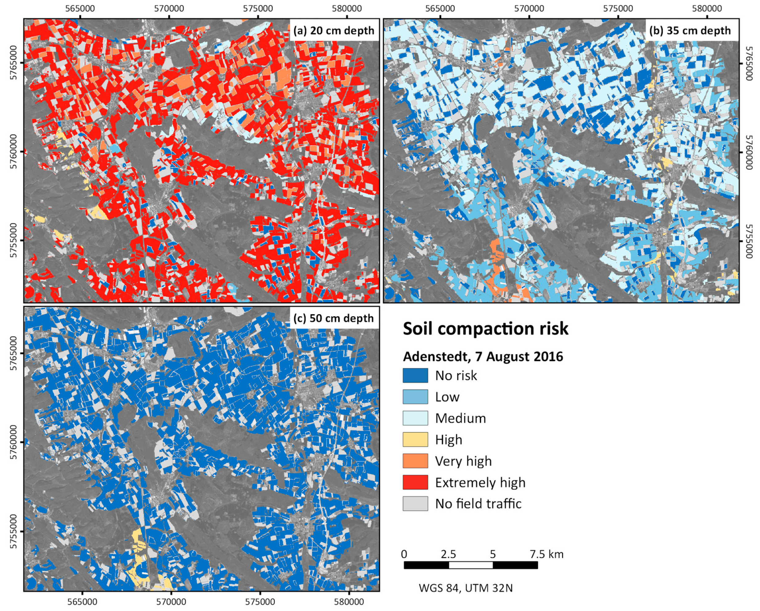
Figure 3 illustrates the spatial distribution of soil compaction risk in three different depths at Adenstedt on 7 August 2016 as modelled with SaSCiA. Table 8 summarizes the area percentage for each compaction risk class and each of the four crop types. The selected depths are 20 cm (topsoil), 35 cm (soil directly beneath the maximum tillage depth) and 50 cm (subsoil).
On 7 August 2016, field traffic potentially affected 80.13% (Table 8) of the total arable area at Adenstedt. The areas covered by maize (10.36%) and rapeseed (9.51%) were not endangered through soil compaction since no field traffic activity took place at this time.
In 20 cm depth, 73.52% showed “high” to “extremely high” risk. Only 3.99% were classified as “no risk” during field traffic activity. The prevailing red colors in Figure 3a clearly demonstrate the high share of areas classified as “high” to “extremely high”. Bluish areas (“no risk” to “medium” risk) were distributed over the entire study area without showing any spatial pattern.
In 35 cm depth, the area proportions changed; only 2.30% of the total area, which related entirely to “cereals”, was classified as “high” or “extremely high”. The percentage area classified as “no risk” during field traffic increased up to 21.12%. Figure 3b highlights the shift with predominating bluish tones, especially light blue. Two regions with higher soil compaction risk are prominent, i.e., a region with “very high” soil compaction risk in the southwestern part and an area with “high” soil compaction risk along a north-to-south corridor in the East.
In 50 cm depth, most of the arable area (78.90%) showed “no risk”; only 1.12% was classified as “high”. Dark blue colors therefore predominate in Figure 3c except in a region in the southwest with “high” and some fields in the northwest with “low” soil compaction risk.
The spatial detail of the soil compaction risk maps depends on the spatial resolution of the soil and crop type data used for soil moisture modelling. The spatial resolution of crop type mapping was 20 m (Adenstedt) and 30 m (Kummerow). As field sizes are often several hectares, the spatial resolution of the crop type information was sufficient for the soil compaction risk assessment. The soil map used in the study area, however, was only available at a scale of 1:200,000. Hence, the spatial distribution of soil properties is highly aggregated and small-scale variations in soil properties remain disregarded. Using a more detailed soil map within SaSCiA-model may enable a more differentiated soil compaction risk assessment.
4.2. Temporal Variation of Soil Compaction Risk
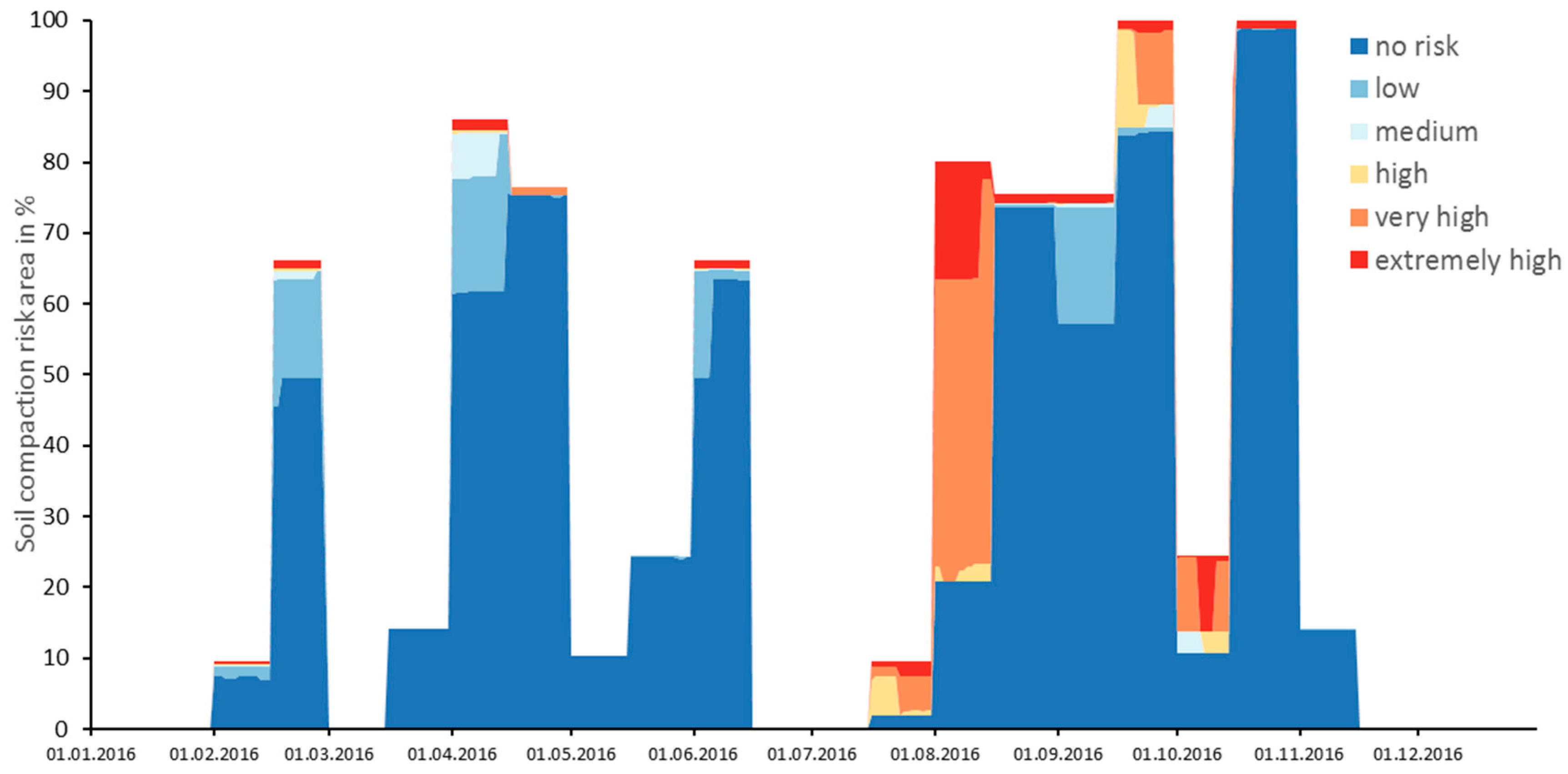
The spatial distribution of soil compaction risk for individual days enables the analysis of the temporal variation for an entire year. Temporal changes of soil compaction risk depend on weather conditions, related crop growth and varying wheel loads. Figure 4 illustrates an example for different depths (20, 35 and 50 cm) at Adenstedt. The area percentage of the individual soil compaction risk classes (ordinate) is highlighted for each day in 2016 (abscissa).
The percentage area affected by field traffic varied between 0% and 100% for arable land throughout the year. No field traffic occurred during winter (January, second half of November and December), in the first half of March and from mid-June to mid-July leading to 0% affected area. During the second half of September and second half of October, field traffic affected the entire arable area, i.e., 100%. During the remaining months, the percentage varied between 9.8% and 85%.
Figure 4 depicts strong leaps of the percentage of soil compaction risk area between certain dates, e.g., 9.5% on 31 July 2016 and 80% on 1 August 2016. These sharp transitions marked the edges of field traffic periods defined in SaSCiA prior to the model run and depend on the particular crop type. This explains, why the area percentage of soil compaction risk at a given date remained the same for all depths (Figure 4a–c), while the share of the soil compaction risk classes varied at the different depths.
For the topsoil (20 cm), the SaSCiA-model revealed the highest soil compaction risk with a high proportion of “high” and “extremely high” risk classes throughout the year. During spring, almost each field traffic activity resulted in an “extremely high” soil compaction risk. In November, each field traffic activity resulted in “high” and “very high” soil compaction risk. In spring and autumn, the high percentage of “high” risk area resulted from high soil moisture. In northern Germany, most precipitation occurs from November to March, while plant transpiration is very low. The wet soil therefore has a low soil strength and is unable to withstand the applied stresses, even of low wheel loads. In summer, the amount of precipitation is low, while plant transpiration rate is high. Soil strength increases with decreasing soil moisture, resulting in a reduced soil compaction risk. Accordingly, the percentage of soil compaction risk classes “low” and “no risk” increased at the beginning of August. Nevertheless, Figure 4 shows that a high percentage of fields remained highly exposed to soil compaction in summer and early autumn. At this time, the harvest activities led to highest wheel loads (5000–10,000 kg), causing soil pressures that exceeded the soil strength even of dry soils.
Below the tillage depth (35 cm) and in the subsoil (50 cm), the soil compaction risk was low for the entire cropping season. At a depth of 35 cm, “no risk” areas predominated. From February to the end of June, SaSCiA revealed a “high” or “extremely high” soil compaction risk only for 3% of the arable land. “Low” to “medium” classes shared 23%. The majority of the trafficked area, however, showed “no risk”. During the first half of August, only 3% were classified as “high” and “very high”, 55% were classified as “low” to “medium”. From the second half of August until the end of the year, all field traffic activities resulted in “no risk” of soil compaction. At a depth of 50 cm, the soil compaction risk decreased continuously compared to the depths at 35 cm. The class “extremely high” never occurred; classes “high” and “very high” had a maximum of 2%. Soil compaction risk classes “low” and “medium” resulted in a maximum of 7%. The majority of field traffic activities were classified as “no risk”. The low soil compaction risk in autumn contradicts the expectation that maize and sugar beet harvest cause the highest soil compaction as reported by e.g., Nevens and Reheul [72], Peth et al. [13] and Destain et al. [40]. In 2016, precipitation sum from July to September was 50% lower (93.2 mm) compared to long-term measurements (184.7 mm) [50]. The low precipitation led to dry soils especially in the subsoil. The dry soil compensated most of the applied soil pressure in the topsoil, resulting in a less affected subsoil.
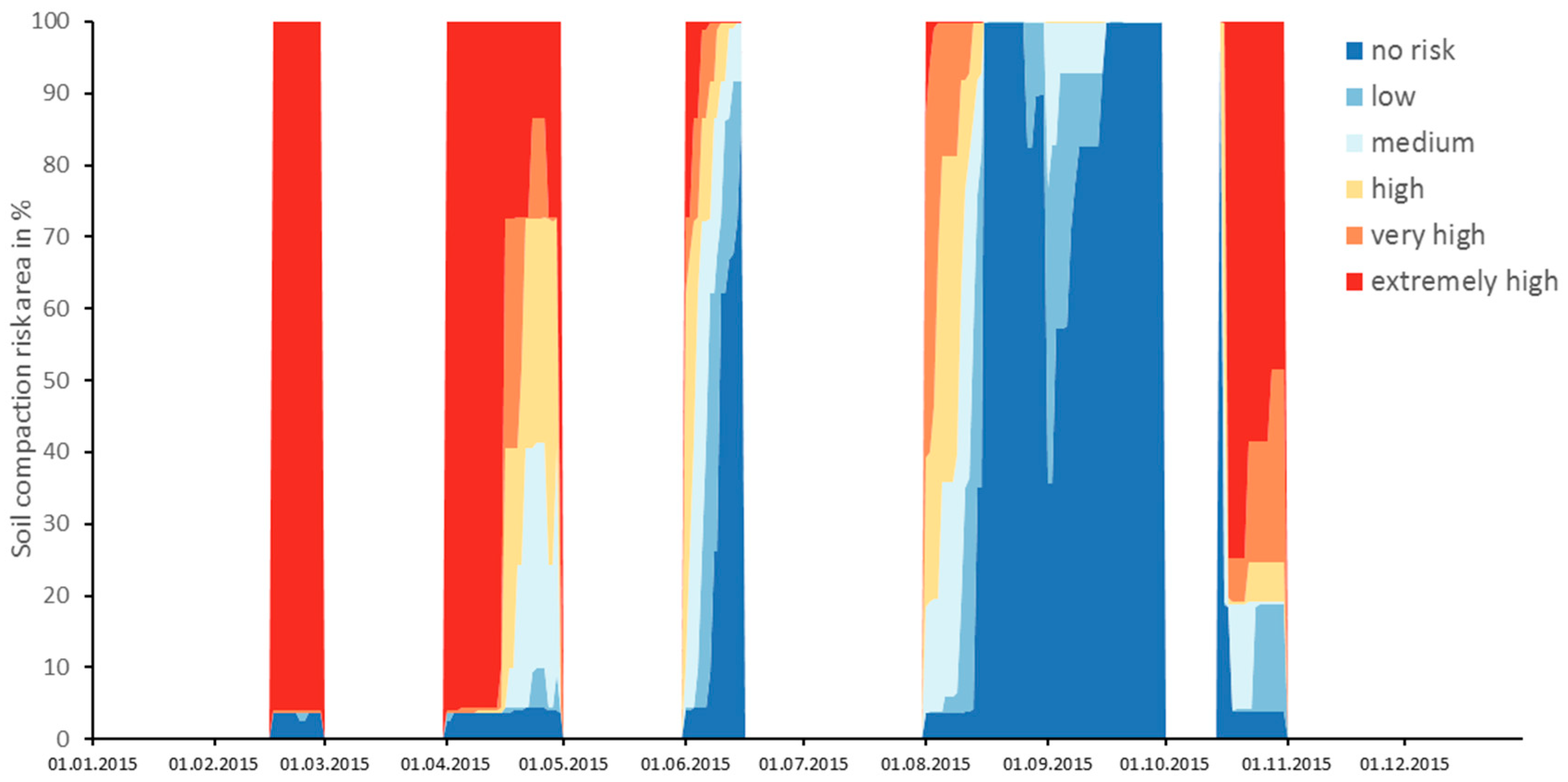
To demonstrate the influence of weather conditions, the soil compaction risk assessment for Adenstedt was repeated with the weather data from 2014. In 2014, precipitation sum was 240.6 mm [50] from July to September representing a year with wet soil conditions during harvest. All other input data remained the same for this scenario. Figure 5 shows the results of the wet scenario at a depth of 35 cm: a clear increase in soil compaction risk for harvest times (16 July to 15 August 2016 and 16 September to 15 October2016) emphasizes the effects of high wheel loads during wet soil conditions compared with dry soil conditions in Figure 4. The results of the wet weather scenario are in agreement with the findings of the former mentioned studies [13,40,72]: high wheel loads during maize and sugar beet harvest increase soil compaction risk.
4.3. Spatio-Temporal Variation for Single Crop Types
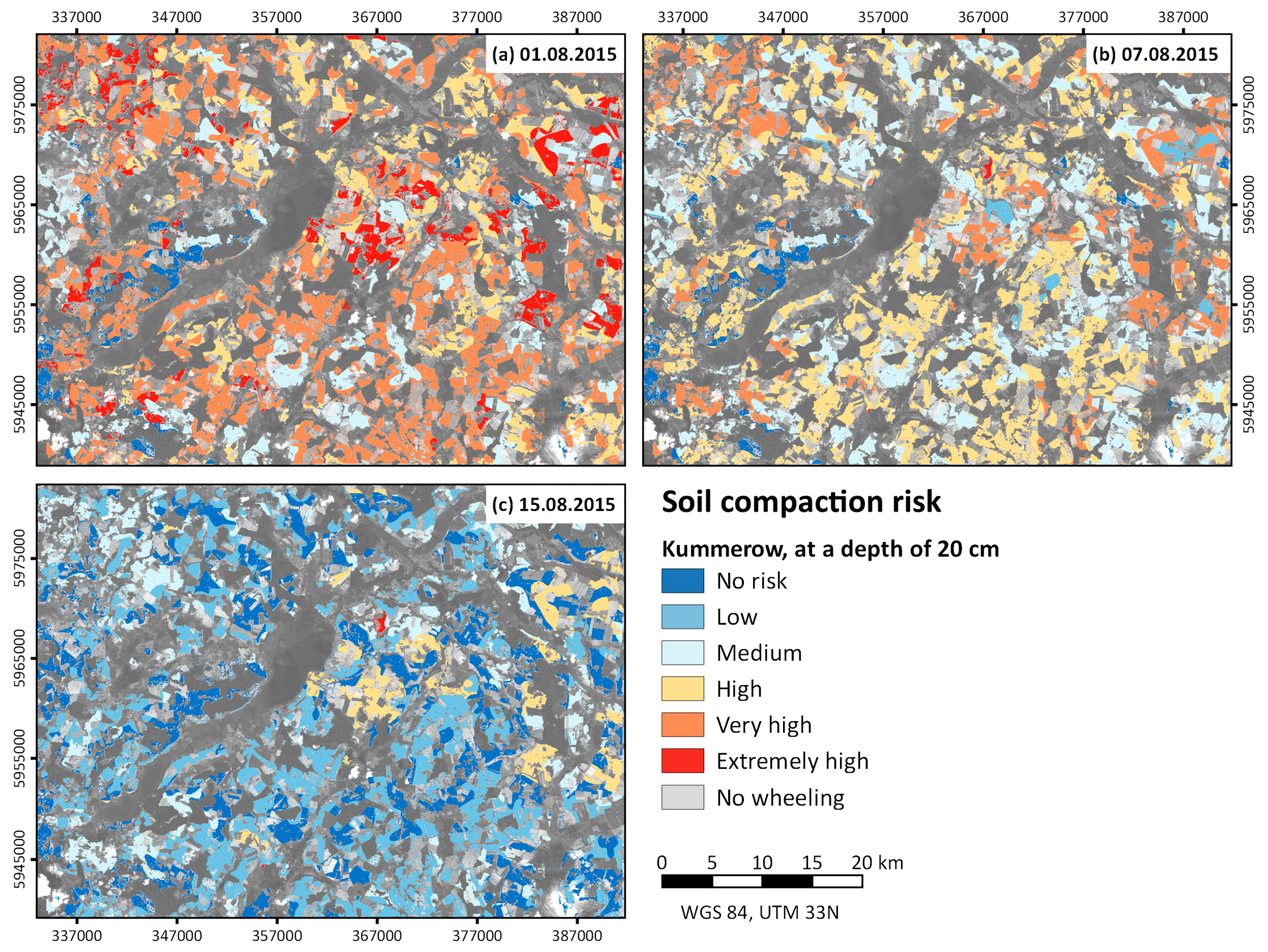
The SaSCiA-model enables analyses of varying soil compaction risk for single crop types. Selecting only one crop type (e.g., sugar beet) enables the analysis of varying soil properties on soil compaction risk. Figure 6 shows an example of the temporal dynamics in soil compaction risk at a depth of 20 cm for areas cultivated with cereals at Kummerow in 2015.
Since cereals was the focused crop type and SaSCiA considers similar field traffic for one crop type, the area affected by field traffic activity was either 0% (no field traffic) or 100% (field traffic on all cereal cultivated areas). Six periods had no field traffic activity. During the year, however, all soil compaction risk classes occurred, whereas spring and autumn showed the highest soil compaction risk. Changes in soil compaction risk classes became apparent within a traffic period. As an example, Figure 7 shows the changes in soil compaction risk during the cereal-harvest period (1 August 2015–15 August 2015) in the Kummerow area.
At the beginning of the harvest period (Figure 7a; 1 August 2015), soil compaction risk was heterogeneously distributed, whereas classes “high” to “extremely high” (81.52%) predominated. Only 3.67% of the area showed “no risk” and 14.81% “low” to “medium” soil compaction risk. Rainy days in July (precipitation sum of 72.4 mm; DWD) caused an increased soil moisture with decreased soil strength. In the following days, however, the desiccating soil led to a decreasing soil compaction risk in the entire region.
On 7 August 2015 (Figure 7b), “low” to “medium” soil compaction classes increased to 32.02%, while “high” to “extremely high” decreased to 64.27%. On 15 August 2015 (Figure 7c), the majority of the trafficked area (57.58%) was classified as “no risk”. Only 7.30% remained with “high” to “extremely high” soil compaction risk class.
The analysis of the cereal-harvest in the Kummerow area (Figure 7) demonstrated how weather conditions may influence the spatial distribution of soil compaction risk on short term. Furthermore, the different soil compaction risk classes for a particular day highlighted the influence of varying soil properties; as crop type, weather information and machinery setup were the same for the entire region, the spatio-temporal variations in soil compaction risk result from different soil conditions.
4.4. Advances and Limitations of the SaSCiA-Model
The applicability of the SaSCiA-model has been demonstrated for two study areas in Germany with different spatial extent and varying land cover, pedological characteristics and weather conditions. The study highlights that the SaSCiA-model generates daily maps of soil compaction risk, which can support a sustainable field management and field traffic strategies to maintain various environmental functions of soils. The potential applications of the SaSCiA-model are manifold:
(i) Real-time soil compaction risk assessment
The SaSCiA-model enables a real-time soil compaction risk assessment, if sufficient data (especially weather and crop type data) is available. Currently available spatial soil compaction models show only the potential soil compaction risk, which is of limited importance for decision-making under real field conditions. The spatio-temporal high-resolution maps produced by SaSCiA show areas with varying (time and space) soil compaction risk. SaSCiA, therefore, can be potentially used as communication and visualization tool. Thus, the up-to-date soil compaction risk maps may support farmers, stakeholders and consultants in making decision for a more sustainable agriculture.
(ii) Retrospective soil compaction risk assessment
The SaSCiA-model is also applicable for retrospective soil compaction risk assessments, as demonstrated in the case studies. As long as crop type information is available (e.g., derived from field mappings or from remote sensing data), the SaSCiA-model can be used to obtain retrospective daily soil compaction risk maps for the last year, decade or even longer (the Landsat archive provides data back to the 1980s). Additional information of former crop types derived by farmers or public institutions may also contribute to generate typical crop rotations for study areas and, therefore, long-term analyses of soil compaction risk.
(iii) Hot-spot detection
The continuous application of the model for several years may identify areas with high soil compaction risk year by year. This hotspot identification may help to prevent further soil compaction by means of adapted field cultivation. Since soil compaction reduces the infiltration rate and increases runoff, detected hot-spot areas may be subject to further investigations, e.g., regarding risk assessment of soil water erosion. Accordingly, Alaoui et al. [7] recently published a review in which they advise the use of remote sensing and new methods of soil compaction mapping for flood analysis and flood prevention. The SaSCiA-model may contribute to this recommendation.
(iv) Deriving days of trafficability
Apart from the assessment of soil compaction risk, the SaSCiA-model may be used to calculate the maximum wheel load day-by-day until no risk (or low or medium risk) occurs. Such analyses, for instance, may provide recommendations to farmers on the maximum payload during harvesting.
(v) Scenario calculations
The study shows that the SaSCiA-model can also be used for scenario calculation. Incorporating modified weather data further enables the analysis of climate change on soil compaction risk. This may help to develop strategies for future machinery setup, field traffic behavior or crop type selection. Effects of crop types on soil compaction risk may be investigated by changing present crop types, e.g., winter wheat instead of maize. This may be of particular interest in regions with changing cultivation practices as observed in Germany; here, the amount of area cultivated with maize extremely increased in the last decade [73,74]. Since maize is one of the crop types causing highest soil compaction risk due to harvest in autumn under wet soil conditions, applying SaSCiA (present crop type (maize) versus an assumed crop type (e.g., winter wheat)) demonstrates changing soil compaction risks under different crop type cultivation.
The forecasting ability of the SaSCiA-model, however, depends on the quality and availability of input data and the assumptions necessary for a regional analysis. In addition, some limitations of the SaSCiA-model must be taken into account:
(i) Crop type detection
The crop type is a key factor for soil compaction risk assessment. Without spatially explicit crop type information, SaSCiA is unable to calculate the soil moisture; related field traffic activities and wheel loads therefore cannot be assigned. To calculate real-time or near real-time soil compaction risk maps, present crop types are required. The availability of freely available crop type data, however, is limited, especially for the present year.
For the two study areas, Sentinel-2A and Landsat 8 satellite data accompanied by field mappings served as input for the crop type mappings. Nevertheless, satellite remote sensing data allow a retrospective assessment; it may also help to identify crop type for the present years. Separation of crop types using remote sensing further depends on their spectral variability, i.e., the spectral signatures must differ significantly at the acquisition day of the satellite. Furthermore, the spectral variability within a crop type has to be lower that the spectral variability between crop types.
During summer months, matured rapeseed may have a similar spectral behavior as cereals; during spring, rapeseed is in full bloom and differs significantly from cereals. After sowing in spring, both maize and sugar beets depict a similar spectral behavior as bare soil; consequently, they are spectrally easier to distinguish in late summer. After maize harvest, it is difficult to distinguish winter wheat as a subsequent crop and yellow mustard as catch crop, or weed growth. In general, images acquired directly after harvest or after sowing tend to impede an accurate crop type classification.
Moreover, the spectral/radiometric characteristics of the satellite sensors determine whether and which crop types can be identified [75,76]. Using satellite remote sensing for real-time crop monitoring therefore may be limited. Land use classifications using remote sensing data in spring or early summer, however, enable an assessment for the following harvest period. Using a series of land cover classifications for several consecutive years, typical crop rotations may also be derived (e.g., [69]). Applying this crop rotation scheme allows a prediction of the following crop type, which then enables a soil compaction risk assessment for the subsequent year.
(ii) Assumptions for input-data
In SaSCiA, the spatial pattern of soil compaction risk results from spatially varying soil properties, crop types and derived soil moisture. Weather information, machinery information and field traffic days are assumed as constant values within the entire region.
For wheel load and tire inflation pressure, one value for each crop type and type of field traffic (e.g., sowing, spraying and harvest) can be specified. If more than one piece of machinery works in the field at the same time, e.g., during maize harvest, only one wheel load can be used for soil compaction risk assessment. In the case studies, the maximum wheel load, i.e., the worst case, was chosen. This may result in an overestimation of soil compaction risk, as wheel load changes dynamically; during sugar beet harvest, for instance, wheel load varies between the empty gross weight of 30 t and a fully loaded weight of 60 t. Some studies therefore focus on changes in wheel load at field scale (e.g., [29,77]). At regional scale, however, the wheel load affecting each raster cell remains unknown. Each part of a field may potentially be wheeled with the maximum load; hence, each raster cell may be affected with a maximum soil compaction risk. In SaSCiA, however, the wheel load and tire inflation pressure is user defined; it therefore depends on the user, which may also select the minimum or the average wheel load.
Due to a lack of information on the distribution of field traffic, the SaSCiA-model neglects rollover frequency. The number of wheel passages, however, affects soil functionality. Each wheel passage leads to a decrease of soil functions (e.g., [78]). Highest field traffic intensity occurs in the headlands (turning areas of the field) and the tramlines [77,79]. The position of tramlines and headlands is highly variable, depending e.g., on field geometry and working width, which aggravates considering its effects at a regional scale. Since each raster cell could potentially be trafficked, any raster cell may be susceptible to soil compaction. Some studies therefore focus on the prediction of field traffic distribution based on field geometry and used machinery setup (e.g., [80]). If these models are further developed, integration into the SaSCiA-model may overcome the disadvantage of missing rollover frequency.
The exact days of field traffic activity is another parameter, which is difficult to consider at a regional scale. The period for e.g., maize sowing lies within a range of weeks and the exact date of sowing depends on the farmer’s decision. The SaSCiA-model therefore integrates periods for each field traffic operation to consider varying field traffic days. The real field traffic activity will most likely occur within the specified period resulting in a reliable soil compaction risk assessment. If available, exact field traffic days can be used.
Another important point is the assumption of static characteristic of further soil properties, for instance dry bulk density and soil structure. The highly dynamic change of soil moisture is part of the SaSCiA-model. Further soil properties such as dry bulk density may also vary during the season as a result of drying-wetting, settling after tillage or other processes. The same applies for the effects of root growth after sowing. Roots may change the soil structure and increase the soil strength during the season. A recently published study reviewed possible impacts of vegetation on soil strength and trafficability [81]. These changes are not considered automatically in the calculation of soil strength. However, effects of root/plant growth are considered in the MONICA-model. Thus, root/plant growth is considered in soil moisture calculation and, therefore, in the calculation of moisture dependent soil compaction risk. Apart from seasonal changes of soil properties, field traffic will affect soil properties. For instance, a traffic activity at the beginning of the year (e.g., fertilizer application) may increase the dry bulk density of the trafficked soil. The change in dry bulk density affects the subsequent calculation of soil strength and plant/root development and, therefore, the calculation of soil moisture. As the SaSCiA-model uses the soil properties given in the soil table and calculates the soil compaction risk based on these properties, changes of soil properties as dry bulk density are not considered automatically. A manual change of soil properties is (until now) the only way to consider seasonal, tillage or traffic induced changes in certain soil properties.
(iii) Model validation
Additional work is required to provide a validation of the SaSCiA-model. Model accuracy, of course, depends on the quality of the input data. Soil information, for instance, is an important input for the SaSCiA-model, but is often only available in a low resolution, as was the situation in the case studies. Thus, the soil information is spatially aggregated and the depiction of the soil heterogeneity therefore is limited. This is, however, rather a problem of data availability than of the model itself. The individual components/models of the SaSCiA-model are well established and proven: the ability to calculate the soil compaction risk for two soil moisture contents (pF 1.8 and 2.5) using the approach by Horn and Fleige 2013 [15] at field, regional or higher scale was demonstrated by several studies [23,26,27,28,29]. The MONICA-model was applied in studies to derive soil moisture and winter wheat yield at regional scale [34,41], which indicates its applicability in the SaSCiA-model. Götze et al. [33] and Jacobs et al. [82] successfully applied the approach from Rücknagel et al. [32] to evaluate the soil compaction risk at individual farms.
It is therefore necessary to verify the predicted soil compaction risk resulting from the interaction of the single model components. This requires further fieldwork and soil sampling conducted before and after any field traffic activity, as described by Batey [3]. The maps resulting from SaSCiA-modelling show the heterogeneous soil compaction risk at high spatial and temporal scales, thus enabling the detection of areas for appropriate soil sampling and model validation.
5. Conclusions
The SaSCiA-model enables a region-wide soil compaction risk assessment at a high spatial and temporal resolution. It combines well-established approaches and models [15,32,34,35] with spatially differentiated soil and crop information. Furthermore, the model integrates varying wheel loads, tire inflation pressures and field traffic days. The results are daily maps of soil compaction risk for entire regions in a spatial resolution exceeding already existing approaches. The applicability of the SaSCiA-model has been demonstrated for two study areas; soil compaction risk for both study areas has been calculated for entire years.
By using freely available data and open source software, a broad community of practicing experts, stakeholders and consultants involved in soil protection may apply the SaSCiA-model.
Even if the model has some limitations as discussed, it currently is the only spatial approach concerning spatial and temporal changes in soil moisture, plant growth and wheel loads. Potential applications of the model are manifold and may range from retrospective, through current to potentially future soil compaction risk assessments.
Author Contributions
M.K. designed the study in collaboration with all co-authors. M.K. prepared the figures and wrote the majority of the text with contributions by K.D. M.K. developed the model and conducted data analyses; K.D. prepared and analyzed the remote sensing data. N.O. and R.D. contributed in reviewing and finalizing the manuscript.
Acknowledgments
The authors thank the anonymous reviewers for their commitment and very helpful comments on improving the manuscript. We are grateful to James F. Petersen and Kilian Etter for the linguistic editing. The Federal Ministry of Education and Research (BMBF) supported this study within the framework of the BonaRes-initiative (Grant No.: 031A563C). We acknowledge financial support for publications cost by Land Schleswig-Holstein within the funding programme Open Access Publikationsfonds.
Conflicts of Interest
The authors declare no conflict of interest.
Appendix A

Table A1.
Structure and example of input weather information (date system: yyyy/mm/dd).
| Date | T_min (°C) | T_avg (°C) | T_max (°C) | Precipitation (mm) | Sunhours (h) | Windspeed (m/sec) | Rel_Humid (%) |
|---|---|---|---|---|---|---|---|
| 2014-01-01 | 1.2 | 3.3 | 5.3 | 0.0 | 1.0 | 4.9 | 79 |
| 2014-01-02 | 4.0 | 6.8 | 9.5 | 0.1 | 0.1 | 5.6 | 80 |
| … | … | … | … | … | … | … | … |
Table A2.
Structure and example of input soil data.
| Soil_ID | Hor | Depth_up | Depth_low | Texture | Gravel | Corg | Structure | DBD | AC | FC | AFC | WP |
|---|---|---|---|---|---|---|---|---|---|---|---|---|
| 101000000 | Ap | 0 | 30 | Ut4 | 1.2 | 1.74 | sub | 1.5 | 6 | 40 | 22 | 18 |
| 101000000 | Sw-Al | 30 | 40 | Ut3 | 0 | 0 | sub | 1.5 | 4 | 36 | 24 | 12 |
| 101000000 | Bt-Sd | 40 | 60 | Tu4 | 0 | 0 | pol | 1.7 | 2 | 34 | 12 | 22 |
| 101000000 | Bvt-Sd | 60 | 110 | Tu4 | 0 | 0 | pol | 1.7 | 2 | 34 | 12 | 22 |
| 101000000 | C | 110 | 200 | Ut3 | 0 | 0 | sub | 1.5 | 4 | 36 | 24 | 12 |
| 102000000 | Ap | 0 | 30 | Lu | 7.8 | 6.69 | sub | 1.2 | 11 | 53 | 25 | 28 |
| … | … | … | … | … | … | … | … | … | … | … | … | … |
Soil_ID = unique soil identifier, Hor = name of horizon (German classification), Depth_up = upper depth of the horizon, Depth_low = lower depth of the horizon, Texture = texture class (German classification), Gravel = gravel content in %, Corg = soil organic matter in %, Structure = aggregates, DBD = dry bulk density in g cm−3, AC = air capacity in vol %, FC = field capacity in vol %, AFC = available field capacity in vol %, WP = wilting point in vol %.
Table A3.
Structure and example of input crop unit for MONICA-modelling (date system: yyyy/mm/dd).
| Crop_rotation_ID | Crop | Sowing | Harvest | Tillage | Depth | Year |
|---|---|---|---|---|---|---|
| 101110 | SM | 2014-04-21 | 2014-09-21 | 2014-09-22 | 30 | 2014 |
| 101101 | WW | 2014-10-21 | 2015-08-07 | 2015-09-21 | 30 | 2015 |
| 101101 | WW | 2015-10-21 | 2016-08-07 | 2016-09-21 | 30 | 2016 |
| 102110 | SM | 2014-04-21 | 2014-09-21 | 2014-09-22 | 30 | 2014 |
| 102101 | WW | 2014-10-21 | 2015-08-07 | 2015-08-08 | 30 | 2015 |
| 102114 | RS | 2015-08-09 | 2016-07-21 | 2016-09-21 | 30 | 2016 |
| … | … | … | … | … | … | … |
SM = silage maize, WW = winter wheat, RS = rapeseed.
Table A4.
Structure and example of input fertilizer data for MONICA-modelling (date system: yyyy/mm/dd).
Table A4.
Structure and example of input fertilizer data for MONICA-modelling (date system: yyyy/mm/dd).
| Crop_rotation_ID | N | Fertilizer | Date | Incorporation |
|---|---|---|---|---|
| 101110 | 67 | CADLM | 2014-05-10 | 1 |
| 101110 | 108 | AN | 2015-03-07 | 0 |
| … | … | … | … | … |
Table A5.
Structure and example of input field traffic data (date system: yyyy/mm/dd).
| Crop | WL_SW | TIP_SW | Start_SW | End_SW | … | WL_HV | TIP_HV | Start_HV | End_HV | … |
|---|---|---|---|---|---|---|---|---|---|---|
| WW | 1800 | 100 | 2016-10-08 | 2016-10-28 | … | 7000 | 100 | 2016-07-11 | 2016-08-15 | … |
| SBE | 1800 | 100 | 2016-03-21 | 2016-04-10 | … | 10,000 | 100 | 2016-10-01 | 2016-11-07 | … |
| SM | 1800 | 100 | 2016-04-21 | 2016-05-20 | … | 9000 | 100 | 2016-09-15 | 2016-10-15 | … |
| … | … | … | … | … | … | … | … | … | … | … |
WW = winter wheat, SBE = sugar beet, SM = silage maize, WL = wheel load, TIP = tire inflation pressure, SW = sowing, HV = harvest, start = beginning of field traffic period, end = ending of field traffic period.
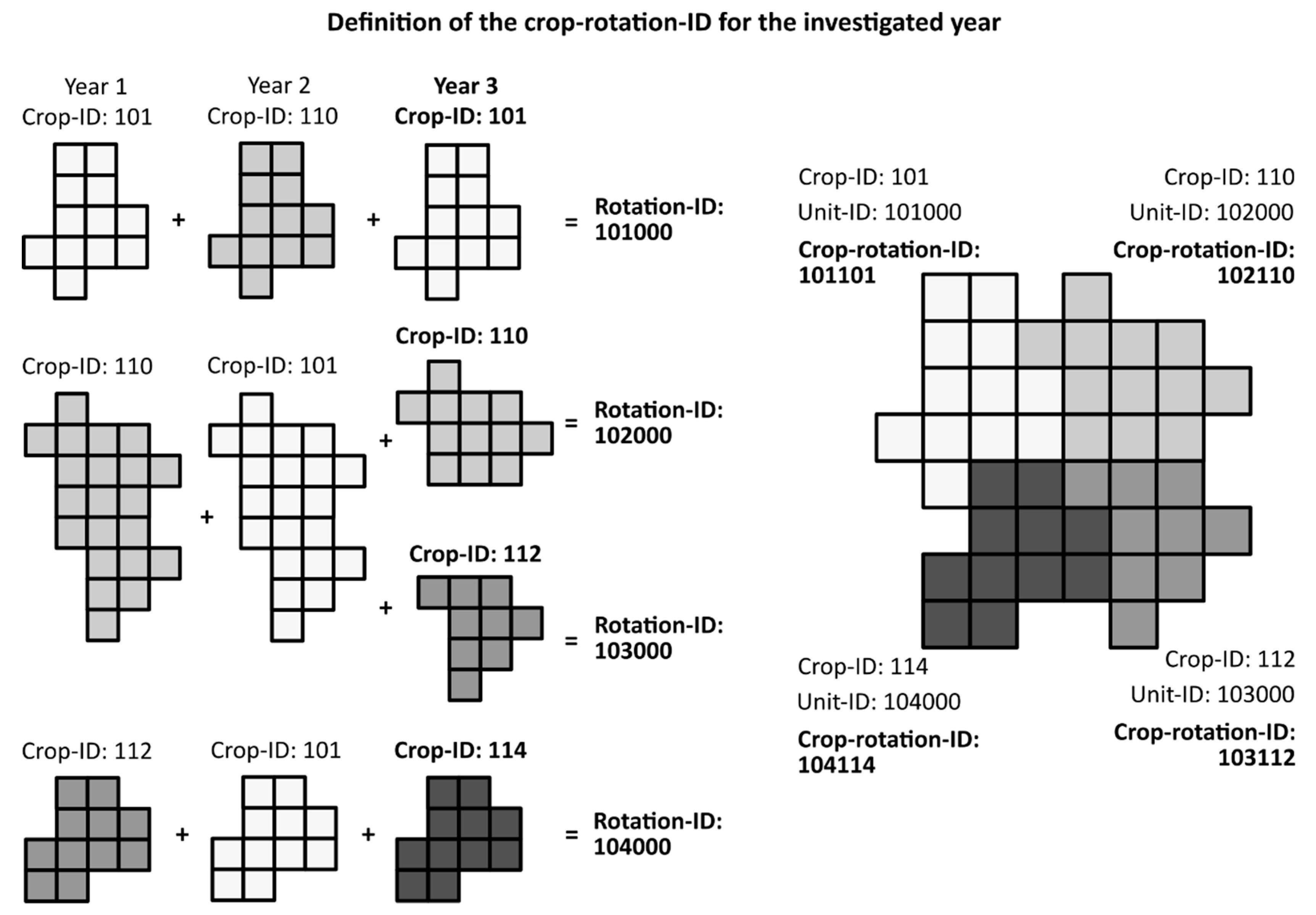
Definition of the Crop-Rotation-ID for the SaSCiA-Model
Figure A1 demonstrates the principle of the creation of “crop-rotation-ID” exemplary. The “crop-rotation-ID” consists of six numbers and contains two information codes. The first three numbers represent the spatial distribution of a crop rotation (“rotation-ID”). The last three numbers represent the present crop type in the investigated year (“crop-ID”).
A crop rotation is a sequence of crop types year by year at the same field/raster cell. The left-hand side of Figure A1 demonstrates the creation of the “rotation-ID”. Each field/raster cell in each year exhibit a crop type (e.g., maize) and is classified by a three-digit number (e.g., 110) based on the classification listed in Table A6. Fields/raster cells with the same sequence of crop types for the three years resulting in a “rotation-ID”. This is the case for the upper and lower examples in Figure A1. The field borders remain unchanged for the period, but crop types vary (101-110-101 and 112-101-114), resulting in two different rotation-IDs (101,000, 104,000). Looking at the example in the middle, the field geometries and crop types are the same for the first two-years. In the third year, the field is subdivided in two different crop types (110 and 112), resulting in two rotation-IDs (102000, 103000). The “rotation-ID” itself is result from a sequential numbering, starting at 101000.
The present crop in the investigated year (year 3) is appended to the rotation-ID. The result is the “crop-rotation-ID”, containing the information of the previous crop type, the present crop type and their spatial distribution (right had side, Figure A1).
Figure A1.
Example of creation of “rotation-ID” and “crop-rotation-ID”.

Table A6.
Crop type, abbreviations and crop-ID for crop types used in the SaSCiA-model.
| Crop Type | Abbreviation | Crop-ID |
|---|---|---|
| Winter wheat | WW | 101 |
| Spring wheat | SW | 102 |
| Winter barley | WB | 103 |
| Spring barley | SB | 104 |
| Winter rye | WR | 105 |
| Spring rye | SR | 106 |
| Winter triticale | WT | 107 |
| Spring triticale | ST | 108 |
| Oat | OA | 109 |
| Silage maize | SM | 110 |
| Grain maize | GM | 111 |
| Sugar beet | SBE | 112 |
| Potato | PO | 113 |
| Rapeseed | RS | 114 |
| Phacelia | PH | 115 |
| Oil radish | OR | 116 |
| Mustard | MU | 117 |
| Broad Beans | BB | 118 |
| Forage peas | FP | 119 |
| Sunflower | SF | 120 |
| … | … | … |
References
- Food and Agriculture Organization (FAO). Status of the World’s Soil Resources: Main Report; FAO, ITPS: Rome, Italy, 2015. [Google Scholar]
- Horn, R.; Domżżał, H.; Słowińska-Jurkiewicz, A.; van Ouwerkerk, C. Soil compaction processes and their effects on the structure of arable soils and the environment. Soil Tillage Res. 1995, 35, 23–36. [Google Scholar] [CrossRef]
- Batey, T. Soil compaction and soil management—A review. Soil Use Manag. 2009, 25, 335–345. [Google Scholar] [CrossRef]
- Gebhardt, S.; Fleige, H.; Horn, R. Effect of compaction on pore functions of soils in a Saalean moraine landscape in North Germany. J. Plant Nutr. Soil Sci. 2009, 172, 688–695. [Google Scholar] [CrossRef]
- Weisskopf, P.; Reiser, R.; Rek, J.; Oberholzer, H.-R. Effect of different compaction impacts and varying subsequent management practices on soil structure, air regime and microbiological parameters. Soil Tillage Res. 2010, 111, 65–74. [Google Scholar] [CrossRef]
- Nawaz, M.; Bourrié, G.; Trolard, F. Soil compaction impact and modelling. A review. Agron. Sustain. Dev. 2013, 33, 291–309. [Google Scholar] [CrossRef]
- Alaoui, A.; Rogger, M.; Peth, S.; Blöschl, G. Does soil compaction increase floods? A review. J. Hydrol. 2018, 557, 631–642. [Google Scholar] [CrossRef]
- Berisso, F.E.; Schjønning, P.; Keller, T.; Lamandé, M.; Etana, A.; Jonge, L.W.D.; Iversen, B.V.; Arvidsson, J.; Forkman, J. Persistent effects of subsoil compaction on pore size distribution and gas transport in a loamy soil. Soil Tillage Res. 2012, 122, 42–51. [Google Scholar] [CrossRef]
- Gut, S.; Chervet, A.; Stettler, M.; Weisskopf, P.; Sturny, W.G.; Lamandé, M.; Schjønning, P.; Keller, T. Seasonal dynamics in wheel load-carrying capacity of a loam soil in the Swiss Plateau. Soil Use Manag. 2015, 31, 132–141. [Google Scholar] [CrossRef]
- Botta, G.F.; Jorajuria, D.; Balbuena, R.; Ressia, M.; Ferrero, C.; Rosatto, H.; Tourn, M. Deep tillage and traffic effects on subsoil compaction and sunflower (Helianthus annus L.) yields. Soil Tillage Res. 2006, 91, 164–172. [Google Scholar] [CrossRef]
- Rücknagel, J.; Christen, O.; Hofmann, B.; Ulrich, S. A simple model to estimate change in precompression stress as a function of water content on the basis of precompression stress at field capacity. Geoderma 2012, 177–178, 1–7. [Google Scholar] [CrossRef]
- Edwards, G.; White, D.R.; Munkholm, L.J.; Sørensen, C.G.; Lamandé, M. Modelling the readiness of soil for different methods of tillage. Soil Tillage Res. 2016, 155, 339–350. [Google Scholar] [CrossRef]
- Peth, S.; Horn, R.; Fazekas, O.; Richards, B.G. Heavy soil loading its consequence for soil structure, strength, deformation of arable soils. J. Plant Nutr. Soil Sci. 2006, 169, 775–783. [Google Scholar] [CrossRef]
- Schjønning, P.; van den Akker, J.J.H.; Keller, T.; Greve, M.H.; Lamandé, M.; Simojoki, A.; Stettler, M.; Arvidsson, J.; Breuning-Madsen, H. Chapter Five—Driver-Pressure-State-Impact-Response (DPSIR) Analysis and Risk Assessment for Soil Compaction—A European Perspective. In Advances in Agronomy; Sparks, D.L., Ed.; Academic Press: Cambridge, MA, USA, 2015; pp. 183–237. [Google Scholar]
- Horn, R.; Fleige, H. A method for assessing the impact of load on mechanical stability and on physical properties of soils. Soil Tillage Res. 2003, 73, 89–99. [Google Scholar] [CrossRef]
- Diserens, E. Calculating the contact area of trailer tyres in the field. Soil Tillage Res. 2009, 103, 302–309. [Google Scholar] [CrossRef]
- Keller, T.; Berli, M.; Ruiz, S.; Lamandé, M.; Arvidsson, J.; Schjønning, P.; Selvadurai, A.P.S. Transmission of vertical soil stress under agricultural tyres: Comparing measurements with simulations. Soil Tillage Res. 2014, 140, 106–117. [Google Scholar] [CrossRef]
- Schjønning, P.; Stettler, M.; Keller, T.; Lassen, P.; Lamandé, M. Predicted tyre–soil interface area and vertical stress distribution based on loading characteristics. Soil Tillage Res. 2015, 152, 52–66. [Google Scholar] [CrossRef]
- Keller, T.; Défossez, P.; Weisskopf, P.; Arvidsson, J.; Richard, G. SoilFlex: A model for prediction of soil stresses and soil compaction due to agricultural field traffic including a synthesis of analytical approaches. Soil Tillage Res. 2007, 93, 391–411. [Google Scholar] [CrossRef]
- Stettler, M.; Keller, T.; Weisskopf, P.; Lamandè, M.; Lassen, P.; Schjønning, P. Terranimo®—A web-based tool for evaluating soil compaction. Landtechnik 2014, 69, 132–138. [Google Scholar]
- Jones, R.J.A.; Spoor, G.; Thomasson, A.J. Vulnerability of subsoils in Europe to compaction: A preliminary analysis. Soil Tillage Res. 2003, 73, 131–143. [Google Scholar] [CrossRef]
- Van den Akker, J.J.H. SOCOMO: A soil compaction model to calculate soil stresses and the subsoil carrying capacity. Adv. Soil Struct. Res. 2004, 79, 113–127. [Google Scholar] [CrossRef]
- Horn, R.; Fleige, H.; Richter, F.-H.; Czyz, E.A.; Dexter, A.; Diaz-Pereira, E.; Dumitru, E.; Enarche, R.; Mayol, F.; Rajkai, K.; et al. SIDASS project: Part 5: Prediction of mechanical strength of arable soils and its effects on physical properties at various map scales. Soil Tillage Res. 2005, 82, 47–56. [Google Scholar] [CrossRef]
- Van den Akker, J.J.H.; Hoogland, T. Comparison of risk assessment methods to determine the subsoil compaction risk of agricultural soils in The Netherlands. Soil Tillage Res. 2011, 114, 146–154. [Google Scholar] [CrossRef]
- DVWK 234. Gefügestabilität Ackerbaulich Genutzter Mineralböden—Teil 1: Mechanische Belastbarkeit; Deutscher Verband für Wasserwirtschaft und Kulturbau: Bonn, Germany, 1995.
- Horn, R.; Fleige, H. Risk assessment of subsoil compaction for arable soils in Northwest Germany at farm scale. Soil Tillage Res. 2009, 102, 201–208. [Google Scholar] [CrossRef]
- Fritton, D.D. Evaluation of pedotransfer and measurement approaches to avoid soil compaction. Soil Tillage Res. 2008, 99, 268–278. [Google Scholar] [CrossRef]
- D’Or, D.; Destain, M.-F. Toward a tool aimed to quantify soil compaction risks at a regional scale: Application to Wallonia (Belgium). Soil Tillage Res. 2014, 144, 53–71. [Google Scholar] [CrossRef]
- Duttmann, R.; Schwanebeck, M.; Nolde, M.; Horn, R. Predicting soil compaction risks related to field traffic during silage maize harvest. Soil Sci. Soc. Am. J. 2014, 78, 408–421. [Google Scholar] [CrossRef]
- Vorderbrügge, T.; Brunotte, J. Vulnerability to compaction of agricultural subsoils—Validation of pedotransfer function for identification of risk areas in Europe and a practicable solution for good farming practice that avoids subsoil compaction, Part I: Validation of pedotransfer function. Appl. Agric. For. Res. 2011, 61, 1–21. [Google Scholar]
- Keller, T.; Arvidsson, J.; Schjønning, P.; Lamandé, M.; Stettler, M.; Weisskopf, P. In Situ Subsoil Stress-Strain Behavior in Relation to Soil Precompression Stress. Soil Sci. 2012, 177, 490–497. [Google Scholar] [CrossRef]
- Rücknagel, J.; Hofmann, B.; Deumelandt, P.; Reinicke, F.; Bauhardt, J.; Hülsbergen, K.-J.; Christen, O. Indicator based assessment of the soil compaction risk at arable sites using the model REPRO. Ecol. Indic. 2015, 52, 341–352. [Google Scholar] [CrossRef]
- Götze, P.; Rücknagel, J.; Jacobs, A.; Märländer, B.; Koch, H.-J.; Christen, O. Environmental impacts of different crop rotations in terms of soil compaction. J. Environ. Manag. 2016, 181, 54–63. [Google Scholar] [CrossRef] [PubMed]
- Nendel, C.; Berg, M.; Kersebaum, K.C.; Mirschel, W.; Specka, X.; Wegehenkel, M.; Wenkel, K.O.; Wieland, R. The MONICA model: Testing predictability for crop growth, soil moisture and nitrogen dynamics. Ecol. Model. 2011, 222, 1614–1625. [Google Scholar] [CrossRef]
- DIN V 19688. Soil Quality—Determination of Compactibilty Risk of Mineral Sub-Soils Based on the Assessed Preconsolidation Stress; DIN: Berlin, Germany, 2011.
- Rücknagel, J.; Götze, P.; Hofmann, B.; Christen, O.; Marschall, K. The influence of soil gravel content on compaction behaviour and pre-compression stress. Geoderma 2013, 209–210, 226–232. [Google Scholar] [CrossRef]
- Koolen, A.J.; Lerink, P.; Kurstjens, D.A.G.; van den Akker, J.J.H.; Arts, W.B.M. Prediction of aspects of soil-wheel systems. Soil Tillage Res. 1992, 24, 381–396. [Google Scholar] [CrossRef]
- R Core Team. R: A Language and Environment for Statistical Computing; R Foundation for Statistical Computing: Vienna, Austria, 2017; Available online: http://www.R-project.org (accessed on 3 March 2017).
- Lamandé, M.; Schjønning, P. Transmission of vertical stress in a real soil profile. Part III: Effect of soil water content. Soil Tillage Res. 2011, 114, 78–85. [Google Scholar] [CrossRef]
- Destain, M.-F.; Roisin, C.; Dalcq, A.-S.; Mercatoris, B.C.N. Effect of wheel traffic on the physical properties of a Luvisol. Geoderma 2016, 262, 276–284. [Google Scholar] [CrossRef]
- Nendel, C.; Wieland, R.; Mirschel, W.; Specka, X.; Guddat, C.; Kersebaum, K.C. Simulating regional winter wheat yields using input data of different spatial resolution. Field Crops Res. 2013, 145, 67–77. [Google Scholar] [CrossRef]
- Specka, X.; Nendel, C.; Hagemann, U.; Pohl, M.; Hoffmann, M.; Barkusky, D.; Augustin, J.; Sommer, M.; van Oost, K. Reproducing CO2 exchange rates of a crop rotation at contrasting terrain positions using two different modelling approaches. Soil Tillage Res. 2016, 156, 219–229. [Google Scholar] [CrossRef]
- Nendel, C.; Specka, X. MONICA—The Model for Nitrogen and Carbon in Agro-Ecosystems. User Manual (Version 1.2.6) 2014. Available online: https://github.com/zalf-rpm/monica (accessed on 28 October 2017).
- Rücknagel, J.; Hofmann, B.; Paul, R.; Christen, O.; Hülsbergen, K.-J. Estimating precompression stress of structured soils on the basis of aggregate density and dry bulk density. Soil Tillage Res. 2007, 92, 213–220. [Google Scholar] [CrossRef]
- Lebert, M. Entwicklung eines Prüfkonzeptes zur Erfassung der Tatsächlichen Verdichtungsgefährdung Landwirtschaftlich Genutzter Böden; UBA-Texte; Ingenieurbüro für Bodenphysik: Dessau-Roßlau, Germany, 2010. [Google Scholar]
- Ad-Hoc-AG Boden. Bodenkundliche Kartieranleitung. 5. Aufl., Hannover; Schweizbart‘sche Verlagsbuchhandlung: Stuttgart, Germany, 2005.
- Food and Agriculture Organization (FAO). World Reference Base for Soil Resources. International Soil Classification System for Naming Soils and Creating Legends for Soil Maps; World Soil Resources Report 106; FAO: Rome, Italy, 2014. [Google Scholar]
- Keller, T. A Model for the Prediction of the Contact Area and the Distribution of Vertical Stress below Agricultural Tyres from Readily Available Tyre Parameters. Biosyst. Eng. 2005, 92, 85–96. [Google Scholar] [CrossRef]
- Söhne, W. Fundamentals of pressure distribution and soil compaction under tractor tires. Agric. Eng. 1958, 39, 276–290. [Google Scholar]
- Germany’s National Meteorological Service (DWD). Available online: https://werdis.dwd.de/werdis/start_js_JSP.do (accessed on 27 March 2017).
- Federal Institute for Geoscience and Natural Resources (BGR). Soil Map at 1:200,000 (BUEK 200). Available online: https://produktcenter.bgr.de/terraCatalog/OpenSearch.do?search=3E80DA1A-A9A7-45A3-9CC7-79796FE9ABA4&type=/Query/OpenSearch.do (accessed on 23 October 2017).
- Wessolek, G.; Kaupenjohann, M.; Renger, M. Bodenphysikalische Kennwerte und Berechnungsverfahren für die Praxis. Bodenökologie und Bodengenese; Technische Universität Berlin: Berlin, Germany, 2009. [Google Scholar]
- Ozdogan, M.; Yang, Y.; Allez, G.; Cervantes, C. Remote Sensing of Irrigated Agriculture: Opportunities and Challenges. Remote Sens. 2010, 2, 2274–2304. [Google Scholar] [CrossRef]
- Calvao, T.; Pessoa, M. Remote sensing in food production—A review. Emir. J. Food Agric. 2015, 138–151. [Google Scholar] [CrossRef]
- Khatami, R.; Mountrakis, G.; Stehman, S.V. A meta-analysis of remote sensing research on supervised pixel-based land-cover image classification processes: General guidelines for practitioners and future research. Remote Sens. Environ. 2016, 177, 89–100. [Google Scholar] [CrossRef]
- Congedo, L. Semi-Automatic Classification Plugin Documentation; Release 5.3.6.1. Available online: https://fromgistors.blogspot.com/p/user-manual.html (accessed on 10 November2017).
- QGIS. A Free and Open Source Geographic Information System. Available online: www.qgis.org (accessed on 15 November 2017).
- Campbell, J.B.; Wynne, R.H. Introduction to Remote Sensing, 5th ed.; The Guilford Press: New York, NY, USA, 2011. [Google Scholar]
- Foody, G.M. Status of land cover classification accuracy assessment. Remote Sens. Environ. 2002, 80, 185–201. [Google Scholar] [CrossRef]
- Immitzer, M.; Vuolo, F.; Atzberger, C. First Experience with Sentinel-2 Data for Crop and Tree Species Classifications in Central Europe. Remote Sens. 2016, 8, 166. [Google Scholar] [CrossRef]
- Kussul, N.; Lemoine, G.; Gallego, F.J.; Skakun, S.V.; Lavreniuk, M.; Shelestov, A.Y. Parcel-Based Crop Classification in Ukraine Using Landsat-8 Data and Sentinel-1A Data. IEEE J. Sel. Top. Appl. Earth Obs. Remote Sens. 2016, 9, 2500–2508. [Google Scholar] [CrossRef]
- Sonobe, R.; Yamaya, Y.; Tani, H.; Wang, X.; Kobayashi, N.; Mochizuki, K.-I. Mapping crop cover using multi-temporal Landsat 8 OLI imagery. Int. J. Remote Sens. 2017, 38, 4348–4361. [Google Scholar] [CrossRef]
- Roy, D.P.; Wulder, M.A.; Loveland, T.R.; Woodcock, C.E.; Allen, R.G.; Anderson, M.C.; Helder, D.; Irons, J.R.; Johnson, D.M.; Kennedy, R.; et al. Landsat-8: Science and product vision for terrestrial global change research. Remote Sens. Environ. 2014, 145, 154–172. [Google Scholar] [CrossRef]
- Drusch, M.; Del Bello, U.; Carlier, S.; Colin, O.; Fernandez, V.; Gascon, F.; Hoersch, B.; Isola, C.; Laberinti, P.; Martimort, P.; et al. Sentinel-2: ESA’s Optical High-Resolution Mission for GMES Operational Services. Remote Sens. Environ. 2012, 120, 25–36. [Google Scholar] [CrossRef]
- Vermote, E.; Justice, C.; Claverie, M.; Franch, B. Preliminary analysis of the performance of the Landsat 8/OLI land surface reflectance product. Remote Sens. Environ. 2016, 185, 46–56. [Google Scholar] [CrossRef]
- European Space Agency (ESA). S2 MPC. Data Quality Report; Reference S2-PDGS-MPC-DQR; Issue 20; Date: 2017-10-05; ESA: Paris, France, 2017. [Google Scholar]
- Müller-Wilm, U. S2PAD SEN2COR 2.2.0—Readme, S2PAD-VEGA-SRN-0001; Telespazio VEGA Deutschland GmbH: Darmstadt, Germany, 2016. [Google Scholar]
- European Space Agency (ESA). The Sentinel-2 Toolbox. Available online: https://sentinel.esa.int/web/sentinel/toolboxes/sentinel-2 (accessed on 20 April 2015).
- Kandziora, M.; Dörnhöfer, K.; Oppelt, N.; Müller, F. Detecting Land Use and Land Cover Changes in Northern German Agricultural Landscapes to Assess Ecosystem Service Dynamics. Landsc. Online 2014, 35, 1–24. [Google Scholar] [CrossRef]
- Achilles, W.; Eurich-Menden, B.; Eckel, H.; Frisch, J.; Fritzsche, S.; Föba, N.; Funk, M.; Gaio, C.; Geebe, S.; Grimm, E.; et al. Betriebsplanung Landwirtschaft 2016/2017. Daten für die Betriebsplanung in der Landwirtschaft; 25 Auflage; KTBL (Kuratorium für Technik und Bauwesen in der Landwirtschaft e.V.): Darmstadt, Germany, 2016. [Google Scholar]
- KTBL (Kuratorium für Technik und Bauwesen in der Landwirtschaft). Leistungs-Kostenrechnung Landbau. Available online: http://daten.ktbl.de/dslkrpflanze/postHv.html (accessed on 8 August 2017).
- Nevens, F.; Reheul, D. The consequences of wheel-induced soil compaction and subsoiling for silage maize on a sandy loam soil in Belgium. Soil Tillage Res. 2003, 70, 175–184. [Google Scholar] [CrossRef]
- Destatis. Statistisches Jahrbuch Deutschland 2006, 1st ed.; Statistisches Bundesamt: Wiesbaden, Germany, 2006. [Google Scholar]
- Destatis. Statistisches Jahrbuch Deutschland 2016, 1st ed.; Statistisches Bundesamt: Wiesbaden, Germany, 2016. [Google Scholar]
- Van Niel, T.G.; McVicar, T.R. Determining temporal windows for crop discrimination with remote sensing: A case study in south-eastern Australia. Comput. Electron. Agric. 2004, 45, 91–108. [Google Scholar] [CrossRef]
- Foerster, S.; Kaden, K.; Foerster, M.; Itzerott, S. Crop type mapping using spectral–temporal profiles and phenological information. Comput. Electron. Agric. 2012, 89, 30–40. [Google Scholar] [CrossRef]
- Duttmann, R.; Brunotte, J.; Bach, M. Spatial analyses of field traffic intensity and modeling of changes in wheel load and ground contact pressure in individual fields during a silage maize harvest. Soil Tillage Res. 2013, 126, 100–111. [Google Scholar] [CrossRef]
- Canillas, E.C.; Salokhe, V.M. Modeling compaction in agricultural soils. Soil Tillage Res. 2002, 65, 221–230. [Google Scholar] [CrossRef]
- Chamen, T.; Alakukku, L.; Pires, S.; Sommer, C.; Spoor, G.; Tijink, F.; Weisskopf, P. Prevention strategies for field traffic-induced subsoil compaction: A review: Part 2. Equipment and field practices. Soil Tillage Res. 2003, 73, 161–174. [Google Scholar] [CrossRef]
- Edwards, G.T.C.; Hinge, J.; Skou-Nielsen, N.; Villa-Henriksen, A.; Sørensen, C.A.G.; Green, O. Route planning evaluation of a prototype optimised infield route planner for neutral material flow agricultural operations. Biosyst. Eng. 2017, 153, 149–157. [Google Scholar] [CrossRef]
- Wieder, W.L.; Shoop, S.A. State of the knowledge of vegetation impact on soil strength and trafficability. J. Terramech. 2018, 78, 1–14. [Google Scholar] [CrossRef]
- Jacobs, A.; Auburger, S.; Bahrs, E.; Brauer-Siebrecht, W.; Christen, O.; Götze, P.; Koch, H.-J.; Mußhoff, O.; Rücknagel, J.; Märländer, B. Replacing silage maize for biogas production by sugar beet—A system analysis with ecological and economical approaches. Agric. Syst. 2017, 157, 270–278. [Google Scholar] [CrossRef]
Figure 1.
Schematic structure of the SaSCiA-model (Spatially explicit Soil Compaction risk Assessment).
Figure 1.
Schematic structure of the SaSCiA-model (Spatially explicit Soil Compaction risk Assessment).
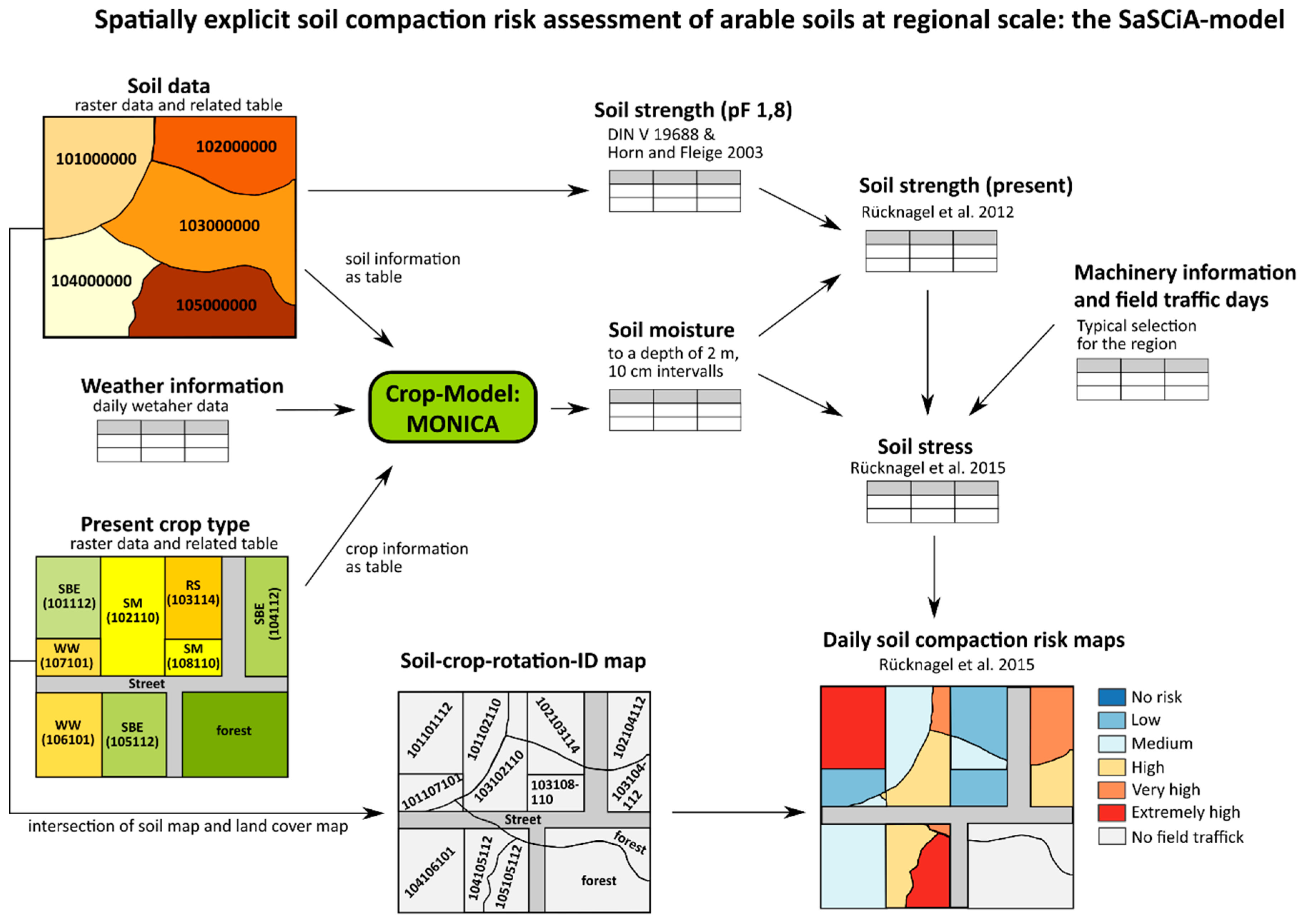
Figure 2.
(a) classification result of Adenstedt based on Sentinel-2A data in the year 2016; (b) classification result of Kummerow based on Landsat 8 data in the year 2015.
Figure 2.
(a) classification result of Adenstedt based on Sentinel-2A data in the year 2016; (b) classification result of Kummerow based on Landsat 8 data in the year 2015.
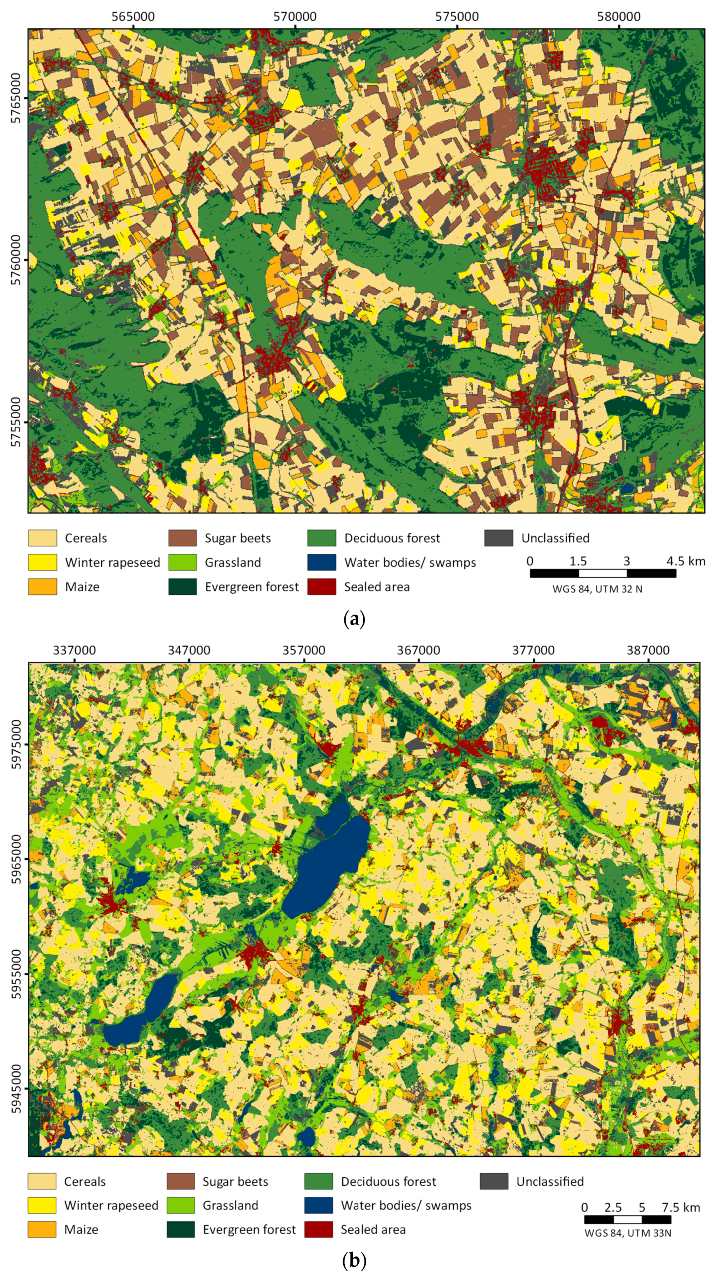
Figure 3.
Soil compaction risk in (a) 20 cm; (b) 35 cm and (c) 50 cm depth at Adenstedt on 7 August 2016).
Figure 3.
Soil compaction risk in (a) 20 cm; (b) 35 cm and (c) 50 cm depth at Adenstedt on 7 August 2016).

Figure 4.
Temporal variation of soil compaction risk for 2016 for (a) 20 cm; (b) 35 cm and (c) 50 cm depth at Adenstedt for 2016. The unit is percentage of the total arable used area. The gap up to 100% represents the percentage area where no field traffic activity occurred on this date (date system: dd/mm/yyyy).
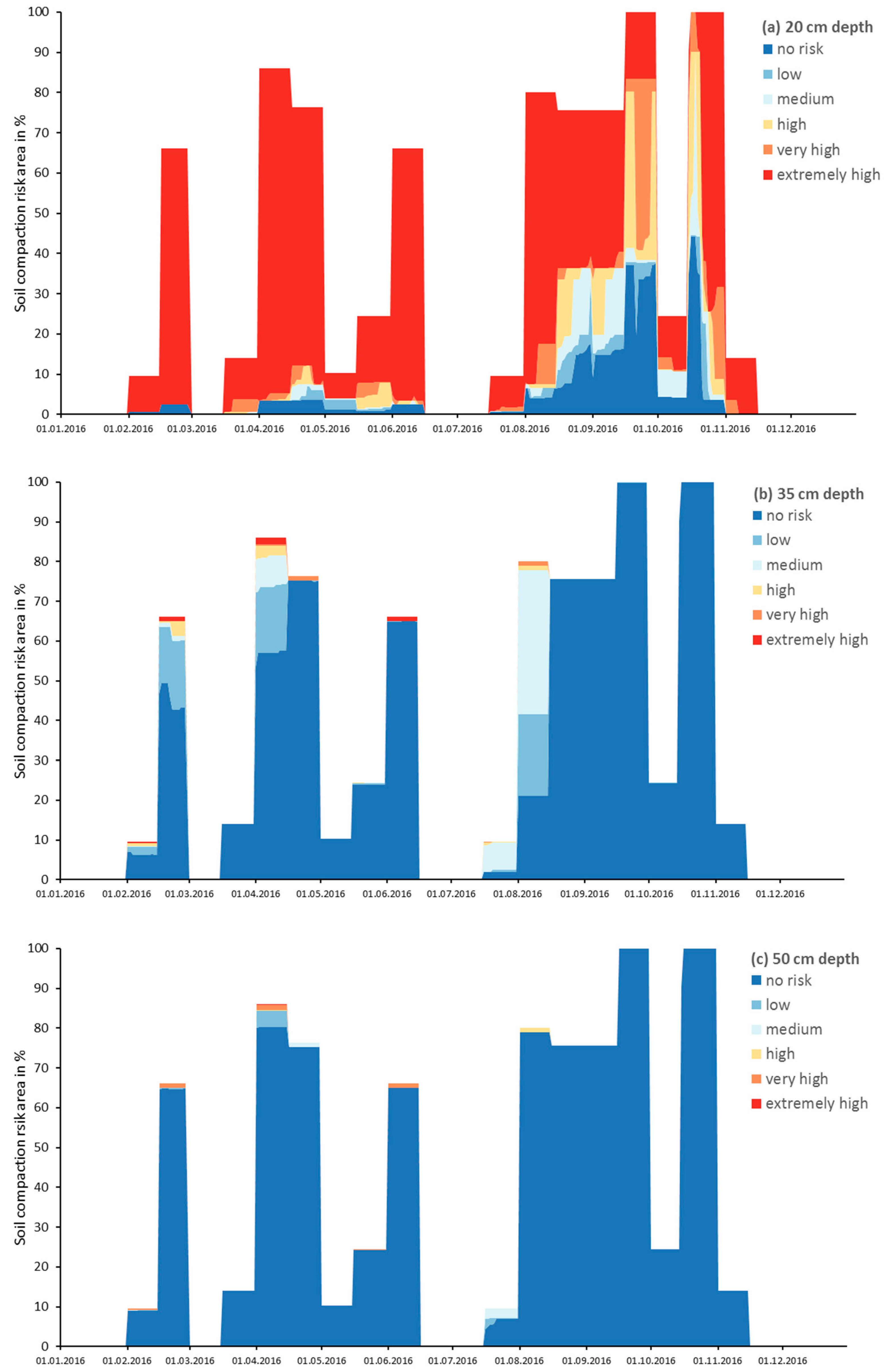
Figure 5.
Temporal variation of soil compaction risk at a depth of 35 cm in Adenstedt for the wet scenario (using weather condition of 2014) (date system: dd/mm/yyyy).
Figure 5.
Temporal variation of soil compaction risk at a depth of 35 cm in Adenstedt for the wet scenario (using weather condition of 2014) (date system: dd/mm/yyyy).

Figure 6.
Temporal variation of soil compaction risk for cereals at a depth of 20 cm at Kummerow (date system: dd/mm/yyyy).
Figure 6.
Temporal variation of soil compaction risk for cereals at a depth of 20 cm at Kummerow (date system: dd/mm/yyyy).

Figure 7.
Soil compaction risk for areas cultivated with cereals at a depth of 20 cm at Kummerow for (a) 1 August 2015; (b) 7 August 2015 and (c) 15 August 2015 (date system: dd/mm/yyyy).
Figure 7.
Soil compaction risk for areas cultivated with cereals at a depth of 20 cm at Kummerow for (a) 1 August 2015; (b) 7 August 2015 and (c) 15 August 2015 (date system: dd/mm/yyyy).

Table 1.
Equations to calculate the soil strength at field capacity (pF 1.8) for varying soil texture class [15,35].
| Formula | Soil Texture Class * |
|---|---|
| (1) σ1.8 = 438.1 × DBD − 0.0008 × Phi3 − 3.14 × WP − 0.11 × AFC2 − 465.6 | Sand (Ss); slightly silty sand (Su2); slightly loamy sand (Sl2); slightly clayey sand (St2) |
| (2) σ1.8 = 69.5 × DBD − 13.3 × Corg − 23.3 × √AC + 1.45 × Coh + 0.085 × Phi2 − 56.6 | medium/highly silty sand (Su3, 4); medium loamy sand (Sl3); silty loamy sand (Slu); silt (Uu); sandy silt (Us); sandy loamy silt (Uls); slightly/medium clayey silt (Ut2, 3) |
| (3) σ1.8 = 119 × DBD − 10.1 × Corg − 12.6 × √WP + 11.1 × √Coh − 78.9 | highly loamy sand (Sl4); highly clayey silt (Ut4); slightly/medium/highly sandy loam (Ls2, 3, 4); silty loam (Lu); highly silty clay (Tu4) |
| (4) σ1.8 = −42.7 × DBD − 20.7 × √Corg − 14.2 × √AFC − 20.8 × √AC + 5.17 × √Phi + 1.23 × √Coh + 231 | medium clayey sand (St3); slightly/medium clayey loam (Lt2, 3); sandy clayey loam (Lts); slightly/medium/highly sandy clay (Ts2, 3, 4); slightly/medium silty clay (Tu2, 3); loamy clay (Tl); clay (Tt) |
* German soil texture classification [46]; σ1.8 = soil strength at field capacity (kPa), DBD = dry bulk density (g cm−3), AC = air capacity (vol %), AFC = available field capacity (vol %), WP = non-plant available water (vol %), Corg = soil organic matter (%), Coh = cohesion (kPa), Phi = angle of internal friction (°).
Table 2.
Equations to calculate the soil moisture depended soil strength for varying soil texture class [11].
Table 2.
Equations to calculate the soil moisture depended soil strength for varying soil texture class [11].
| Formula | Soil Texture Class * |
|---|---|
| (5) log σMoist = 2.8335 + −0.9271 × log σ1.8 + −0.0279 × %FC + 1.67 × 10⁻⁷ × %FC2 + 0.00906 × log σ1.8 × %FC | Sandy Clay, Sandy Clay Loam |
| (6) log σMoist = 2.7833 + −1.0 × log σ1.8 + −0.0278 × %FC + −116 × 10−15 × %FC2 + 0.01 × log σ1.8 × %FC | Loam, Sandy Loam |
| (7) log σMoist = 4.3056 + −1.4444 × log σ1.8 + −0.0431 × %FC + −537 × 10−16 × %FC2 + 0.0144 × log σ1.8 × %FC | Clay, Clay Loam |
| (8) log σMoist = 2.5333 + −0.6667 × log σ1.8 + −0.0253 × %FC + 21 × 10−14 × %FC2 + 0.00667 × log σ1.8 × %FC | Silty Clay Loam, Silty Clay |
| (9) log σMoist = 1.7611 + −0.5556 × log σ1.8 + −0.0176 × %FC + 4.11 × 10⁻¹⁴ × %FC2 + 0.00556 × log σ1.8 × %FC | Sand, Silt Loam, Silt, Loamy Sand |
* USDA soil texture classification [47]; σMoist = soil strength at actual soil moisture (kPa), σ1.8 = soil strength at field capacity (kPa), %FC = actual soil moisture in percent of field capacity (%).
Table 3.
Equations to calculate the effects of gravel on soil strength for varying soil texture class [36].
Table 3.
Equations to calculate the effects of gravel on soil strength for varying soil texture class [36].
| Formula | Soil Texture Class * |
|---|---|
| (10) log σGravel = 0.0434 × e(0.0777 × Gravel) | Clay |
| (11) log σGravel = 0.031 × e(0.083 × Gravel) | Silt Loam |
| (12) log σGravel = 0.0772 × e(0.0631 × Gravel) | Sandy Loam |
* USDA soil texture classification [47]; σGravel = Gravel effect on soil strength (kPa), Gravel = gravel content (%), e = Euler’s number.
| SCI | Soil Compaction Risk |
|---|---|
| ≤0 | No risk |
| 0–0.1 | Low |
| 0.1–0.2 | Medium |
| 0.2–0.3 | High |
| 0.3–0.4 | Very high |
| >0.4 | Extremely high |
Table 5.
Summary on input data for crop type mapping (date system: dd/mm/yyyy)
| Adenstedt | Kummerow | |
|---|---|---|
| Field mapping year | 2016 | 2015 |
| Satellite data | Sentinel-2A | Landsat 8 |
| Atmospheric correction | Sen2Cor | USGS Surface reflectance product |
| Spectral bands (center wavelengths [nm]) | 490, 560, 665, 705, 740, 783, 842, 865, 1610, 2190 | 440, 480, 560, 655, 865, 1610, 2200 |
| Spatial resolution [m] | 20 | 30 |
| Acquisition dates | 2 May 2016, 30 August 2016, 12 September2016 | 10 April 2015, 3 May 2015, 13 June 2015, 23 August 2015 |
Table 6.
Class statistics and accuracy measures of the crop type/land cover classification.
| Adenstedt | Lake Kummerow | |||||
|---|---|---|---|---|---|---|
| Class | Share [%] | PA [%] | UA [%] | Share [%] | PA [%] | UA [%] |
| Unclassified | 15.0 | - | - | 7.8 | - | - |
| Arable land | 44.9 | 49.8 | ||||
| - Cereals | 29.7 | 97.9 | 94.3 | 34.7 | 87.8 | 86.5 |
| - Winter rapeseed | 4.3 | 94.2 | 100 | 10.3 | 80.6 | 86.2 |
| - Maize | 4.7 | 84.4 | 97.3 | 4.5 | 65.3 | 65.7 |
| - Sugar beets | 6.3 | 98.6 | 93.7 | 0.3 | NA * | NA * |
| Non-arable land | 40.1 | 42.3 | ||||
| - Grassland | 2.1 | 56.6 | 82.8 | 16.1 | 93.8 | 81.9 |
| - Water bodies/swamps | 0.1 | 100.0 | 100 | 2.6 | 100.0 | 100 |
| - Evergreen forest | 7.7 | 100.0 | 97.1 | 4.3 | 98.7 | 97.5 |
| - Deciduous forest | 26.5 | 98.1 | 89.6 | 15.6 | 98.8 | 97.5 |
| - Sealed area | 3.7 | 69.8 | 100.0 | 3.7 | 93.1 | 98.5 |
| Overall accuracy [%] | 91.5 | 89.2 | ||||
| Cohen’s kappa | 0.8992 | 0.8741 | ||||
PA = producer’s accuracy is the share of all correctly classified pixels and the sum of all validation pixels of a class; UA = user’s accuracy is the share of all correctly classified pixels and the sum of all classified pixels of a class; overall accuracy is the share of all correctly classified pixels and the sum of all validation pixels; the kappa coefficient additionally includes erroneously classified pixels and considers agreement by chance; * due to rare cultivation in Kummerow area all mapped sugar beet fields were used for classifier training impeding an independent validation.
Table 7.
Machinery setup used for the SaSCiA-modelling for both study area.
| Field Traffic | Machinery | Tractor/Trailer | |
|---|---|---|---|
| max. Wheel Load (in kg) | TIP (in Bar) * | ||
| Primary tillage | Tractor (120 kW) + chisel | 2500 | 0.8 |
| Secondary tillage | |||
| - Maize | Tractor (83 kW) + rotary harrow | 2200 | 1.0 |
| - Sugar beet | Tractor (83 kW) + rotary harrow | 2200 | 1.0 |
| Sowing | |||
| - Cereals, Rapeseed | Tractor (120 kW) + seed drill combination | 1700 | 1.0 |
| - Maize | Tractor (67 kW) + precision seeder | 1800 | 1.0 |
| - Sugar beet | Tractor (67 kW) + precision seeder | 1800 | 1.0 |
| Fertilizer | |||
| - All other | Tractor (83 kW) + mounted spreader (1200 L) | 2400 | 1.6 |
| - Maize | Tractor (120 kW) + slurry tank (14 m3) | 4600 | 2.1 |
| Crop protection | Tractor (67 kW) + trailed sprayer (2500 L) | 1100 | 1.8 |
| Harvest | |||
| - Cereals, Rapeseed | Combine harvester (220 kW, 8300 L) | 8200 | 2.0 |
| - Maize | Self-propelled harvester + tractor + trailer (42 m³) | 5100 | 2.2 |
| - Sugar beet | Self-propelled harvester (390 kW, 22 Mg) | 11,200 | 2.2 |
| Stubble machining | Tractor (120 kW) + disc harrow | 2500 | 0.8 |
* TIP = tire inflation pressure.
Table 8.
Percentage area of soil compaction risk classes at Adenstedt on 7 August 2016.
| Crop | No Field Traffic | No Risk | Low | Medium | High | Very High | Extremely High | Total |
|---|---|---|---|---|---|---|---|---|
| Depth 20 cm | ||||||||
| Cereals | 0.00 | 0.19 | 0.23 | 2.06 | 0.96 | 0.02 | 62.63 | 66.07 |
| Maize | 10.36 | 0.00 | 0.00 | 0.00 | 0.00 | 0.00 | 0.00 | 10.36 |
| Sugar beet | 0.00 | 3.80 | 0.32 | 0.04 | 0.00 | 9.91 | 0.00 | 14.06 |
| Rapeseed | 9.51 | 0.00 | 0.00 | 0.00 | 0.00 | 0.00 | 0.00 | 9.51 |
| Depth 35 cm | ||||||||
| Cereals | 0.00 | 7.06 | 20.42 | 36.29 | 1.07 | 1.23 | 0.00 | 66.07 |
| Maize | 10.36 | 0.00 | 0.00 | 0.00 | 0.00 | 0.00 | 0.00 | 10.36 |
| Sugar beet | 0.00 | 14.06 | 0.00 | 0.00 | 0.00 | 0.00 | 0.00 | 14.06 |
| Rapeseed | 9.51 | 0.00 | 0.00 | 0.00 | 0.00 | 0.00 | 0.00 | 9.51 |
| Depth 50 cm | ||||||||
| Cereals | 0.00 | 64.84 | 0.10 | 0.00 | 1.12 | 0.00 | 0.00 | 66.07 |
| Maize | 10.36 | 0.00 | 0.00 | 0.00 | 0.00 | 0.00 | 0.00 | 10.36 |
| Sugar beet | 0.00 | 14.06 | 0.00 | 0.00 | 0.00 | 0.00 | 0.00 | 14.06 |
| Rapeseed | 9.51 | 0.00 | 0.00 | 0.00 | 0.00 | 0.00 | 0.00 | 9.51 |
© 2018 by the authors. Licensee MDPI, Basel, Switzerland. This article is an open access article distributed under the terms and conditions of the Creative Commons Attribution (CC BY) license (http://creativecommons.org/licenses/by/4.0/).
Share and Cite
MDPI and ACS Style
Kuhwald, M.; Dörnhöfer, K.; Oppelt, N.; Duttmann, R. Spatially Explicit Soil Compaction Risk Assessment of Arable Soils at Regional Scale: The SaSCiA-Model. Sustainability 2018, 10, 1618. https://doi.org/10.3390/su10051618
AMA Style
Kuhwald M, Dörnhöfer K, Oppelt N, Duttmann R. Spatially Explicit Soil Compaction Risk Assessment of Arable Soils at Regional Scale: The SaSCiA-Model. Sustainability. 2018; 10(5):1618. https://doi.org/10.3390/su10051618
Chicago/Turabian StyleKuhwald, Michael, Katja Dörnhöfer, Natascha Oppelt, and Rainer Duttmann. 2018. "Spatially Explicit Soil Compaction Risk Assessment of Arable Soils at Regional Scale: The SaSCiA-Model" Sustainability 10, no. 5: 1618. https://doi.org/10.3390/su10051618
Note that from the first issue of 2016, this journal uses article numbers instead of page numbers. See further details here.