Coupling between Rural Development and Ecosystem Services, the Case of Fujian Province, China
by
 , ,
, ,
Huaxiang Chen
1,2 ,
,
Lina Tang
1,
Quanyi Qiu
1,*,
Tong Wu
1,2,
Ziyan Wang
1,2,
Su Xu
1 and
Lishan Xiao
1 1
Key Laboratory of Urban Environment and Health, Institute of Urban Environment, Chinese Academy of Sciences, Xiamen 361021, China
2
University of Chinese Academy of Sciences, Beijing 100049, China
*
Author to whom correspondence should be addressed.
Sustainability 2018, 10(2), 524; https://doi.org/10.3390/su10020524
Submission received: 24 November 2017
/
Revised: 8 February 2018
/
Accepted: 11 February 2018
/
Published: 15 February 2018
Abstract
:To reveal the relationship between rural development and ecosystem services and to assist in efforts to balance these factors, we used a coupling model to carry out a study of the relationship between rural development and ecosystem services in Fujian Province of China during the years 2000 to 2015. First, we characterized the degree of rural development for each county in the province by calculating its index of relative rurality (IRR) and classified the counties into rural development types. Second, we calculated the values of three ecosystem services (ES) and overlapped them to get the sum of ES for each county. Third, we calculated the coupling and coupling coordination degree and analyzed the correlation between IRR and ES in the study area. The results showed that the mean value of IRR declined over the study period, was positively correlated with ES, and the correlation degree increased year by year. Meanwhile the degree of coupling was in the antagonistic stage, but tended to run in stage with a highly coordinated stage coupling coordination degree, if the business services type-counties were excluded. Although the overall coupling coordination degree was high, it declined yearly, which meant that rural development and ecosystem services increasingly lacked coordination. This paper supports and verifies some achievements of rural development programs in the research area, provides theoretical and decision-making support for coordinated rural development and ecosystem services protection in China, and provides a regional case study that could assist with similar research in other countries.
1. Introduction
Rural areas are complex ecosystems under the simultaneous influences of nature and of social and economic human activities [1], and they play an important role in supplying food, fresh water, and fuel. However, according to the Millennium Ecosystem Assessment (MA) [2], fresh water, air and other natural resources are being degraded or used unsustainably around the world, especially in rural areas [3]. Against the background of rapid urbanization in China, the importance of rural areas to regional development, ecology and food security is even more significant [4]. Rural areas and ecosystems also face the challenges of transformation and development [3]. Research has shown that human societies rely on ecosystem services [5], which include provisioning services, regulating services, supporting services and cultural services [6]. With the rapid advance of urbanization and new rural development, rural social and economic conditions have been greatly improved [7]; however, these changes may lead to a series of new problems. For example, China’s population growth has resulted in degradation or even depletion of ecosystem services [8,9], and resource extraction and environmental pollution have put tremendous pressure on rural ecosystems, leading to dysfunction [10]. The “cancer village” caused by soil and water pollution in Guiyu Shantou, Guangdong Province in China is a representative example.
Rural ecosystem health has gained close attention from governments committed to making improvements, and ecosystem health has become one of the key desired endpoint of environmental management in China in recent decades [11]. Differences between urban and rural areas, changes in agriculture and rural characteristics in the context of globalization, and the reconstruction of sustainable rural landscapes also have become key research fields in international geography [12,13]. Understanding the interactions between rural ecosystems and their underlying environmental constraints, the services they provide, and the people benefiting from those services are essential for the effective management and sustainability of socio-ecosystems [14].
Rurality, a term used to describe the level of rural development, is an important indicator used to reveal differences between villages and identify distinct rural areas [15,16]. Cloke [17,18] and Waldorf [19] are two representative figures in rurality research. Cloke and Edwards [17,18] established a rurality concept system including occupation, population, migration, housing conditions, land use and remoteness, and then used it to calculate the rurality of England and Wales in 1971. Waldorf [19] (2006) believed that the countryside was a multi-dimensional concept, so he selected population, urban built-up area, and degree of remoteness as factors in the calculation of the Index of Relative Rurality (IRR) based on the definition of the Human Development Index (HDI). Zhang [3] (2016), Long [20] (2009), Liang [21] (2016), and other Chinese researchers have constructed rurality evaluation systems that allow one to determine the strength or weakness of rurality in a designated area. However most studies on rural development have concentrated on the path of development, the drivers of development, the flow of population, and social and economic impacts, and few studies have focused on development’s impacts on ecosystem services in the Chinese countryside, according to our literature search on the internet. Existing publications include assessments of rural ecosystem health [1], assessments of the impacts of urbanization on urban ecosystem services [22], and studies of ecosystem services in environmental and land use planning [23].
Coupling, as a concept in physics, refers to a phenomenon in which two (or more than two) systems or forms of motion influence each other through various interactions [24,25]. The coupling degree (C) [24,25] has been used to describe the degree of interaction and influence within a system or among system elements. The coupling degree and a related measure, the coupling coordination degree (D), were therefore used to measure whether the internal elements of system were in harmony with each other in the development process, which reflects the tendency of the system to move from disorder to order [26,27]. Coupling is now widely used in studies of climate change and the environment [25]. In 2005, Liu and Song [28] used the coupling model to study the intensity of interaction between urbanization and the environment. In 2012, Liu and Yang [25] used the coupling model of coordination to research dynamic trends in the development of rapid urbanization and the environment. The maintenance of ecosystem services is essential for sustainable rural development and environmental health [29], and rural industrial activity is the primary driving force for changes in ecosystem services [30], so the interactions between rural development and ecosystems are worthy of study.
In this research, we used coupling models to investigate the relationship between rural development and ecosystem services in Fujian province of China and attempted to answer these questions: (1) Are there interactions among regional rurality, ecosystem services, and types of economic development? (2) How do these factors influence each other? (3) Are these influences beneficial or not? (4) How can we adjust the process of rural development to ensure that ecosystem services are maintained? This research will help decision-makers choose appropriate rural development measures, adjust to local conditions, and seek balance between rural development and the protection of ecosystem services.
2. Data and Methods
2.1. Research Area and Data Sources
To explore characteristics and trends in rural development and ecosystem services, this paper took Fujian Province as the research area, based on the availability of data. We took the administrative division in 2015 as a basis and designated 84 districts, counties, county-level cities, or autonomous counties as basic analysis units. The study period was from 2000 to 2015, with every five years as a time node. The statistical data comes from the Fujian Statistical Yearbook 2000–2015 editions [31], the land use data comes from the Resources and Environment Science Data Center, Chinese Academy of Sciences [32], and the meteorological data comes from the China Meteorological Data Network [33].
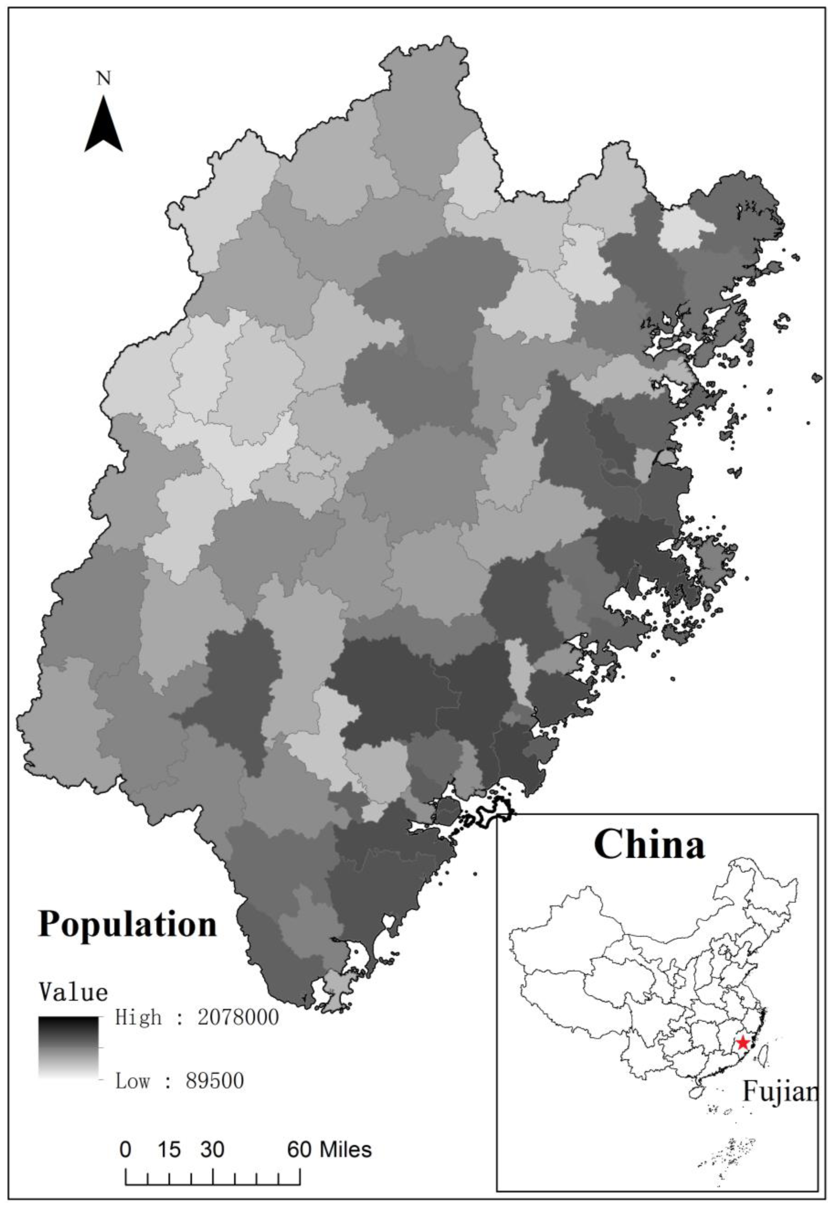
Fujian Province is located on the southeast coast of China. The administrative area of the province is about 124 thousand square kilometres, of which urban area accounts for 33% and rural area accounts for 67% (The location of Fujian in China is as follow Figure 1). In 2015, 37.4% of the population resided in rural areas. The regional GDP per capita was 679,000 yuan (1 Chinese yuan ≈ 0.16 US dollar), higher than the national average, and the level of urbanization (urban population/total population) was 62.6%. In 2000, the output value of secondary industry in research areas accounted for 43.26% of GDP, 50.29% in 2015. However, the contribution rate decreased from 59.6% to 46.6%, which meant the contribution of secondary industry to economic growth was decreased. The tertiary industry accounted for 39.73% of the total economic output value in 2000 and 41.56% in 2015, while the contribution rate increased from 35.7% to 50.5%. By contrast, the primary industry accounted for 17.22% of GDP in 2000 8.15% in 2015, and the contribution rate decreased from 4.7% to 2.9% (Table 1).
Fujian was formerly the most underdeveloped region in the entire country and was the frontier region for China’s opening-up reform program. Fujian underwent rapid development during the years 2000–2015. Fujian has been used as a rural tourism test base as it features beautiful countryside, unique ecological villages in which soil and water are conserved, and vibrant folk culture such as in the township of Hakka. The countryside of Fujian has developed rapidly, and the provincial government has implemented plans for new towns, characteristic villages, integrated rural tourism, leisure and ecological agriculture.
2.2. Methods
2.2.1. Index of Relative Rurality
The Index of Relative Rurality (IRR) has been used to depict the degree of rural development, with greater IRR values indicating stronger rurality and a lower degree of urbanization. Previous research from our group used Waldorf’s [19] (2006) IRR method to reveal the degree of development and characteristics of a rural area. For this study, we selected population size, population density, proportion of area of construction and degree of remoteness as four indicators, and with each indicator given the same weight, we calculated the county’s IRR in the research area during the period 2000–2015. The calculation method was as follow [34]:
In Formula(1), stands for each county’s population size; stands for population density; stands for proportion of area of construction and stands for degree of remoteness. The degree of remoteness is defined as the minimum distance from the research area’s geometric center to the nearest urban area’s geometric center, as calculated through ArcGIS tools. The population size, population density and proportion of area of construction were negative indicators and the degree of remoteness is a positive indicator.
We calculated each county’s IRR over four periods during 2000–2015, and used an expert scoring method based on the results of previous studies to categorize the IRR values into five levels: very weak, weak, moderate, strong, and very strong [35], as shown in Table 2. In order to better show these differences in detail, we spatially mapped the categories using an equal interval method on ArcGIS.
As is the standard practice, the rural development type [36] was characterized by the proportion of GDP accounted for by each broad industry category. Since the standard deviation value can reflect the degree of dispersion of a data set, if the relative proportion of the output value of an industry exceeds the sum of the mean value and standard deviation value of whole samples, it shows that the industry occupies the leading position in local economic development [20]. We partitioned the development type of 84 counties in Fujian Province by calculating the percentage contribution of each industry’s output value to the region’s total economic output, then categorized the counties based on whether the proportion was greater than the sum of standard deviation value and the mean value of all the samples (Table 3). If none of the proportions (GDP1, GDP2, GDP3) are higher than the sum of standard deviation value and the mean value of all the samples, the county is categorized as belonging to the balanced development type. Thus, in this paper, the balanced development type means that agriculture, industry and business services coexist in a county, and no one of these is the leading industry.
2.2.2. InVEST Models
The Integrated Valuation of Ecosystem Services and Tradeoffs Tool (InVEST) was developed by the Natural Capital Project [37]. It is a comprehensive suite of models used to quantify and value ecosystem services (ES); it has been applied in North America, China and other regions and has provided some useful simulation results under different land use change and development scenarios [37]. One advantage of using the InVEST models to calculate ecosystem services is that the results can be directly used to analyse the spatial distribution and heterogeneity of an ecosystem service. Additionally, the protection of natural resources and the relationship between natural resources and economic development can be weighed using the model’s scenario simulations and comparisons of ecosystem service gains and losses, which can assist decision makers by providing a scientific basis for decision-making [9].
In this study, based on the availability of basic data, we chose to investigate three ecosystem services, carbon storage, habitat quality, and annual water yield, which represented a regulating service, a support service and a provisioning service, respectively. Since the calculation processes used in InVEST models are complex, the data requirements and model operations are not described in detail in this paper. Detailed methods and the manual for InVEST models are available at the InVEST website, https://www.naturalcapitalproject.org/invest/. Briefly, the calculation methods are as follows:
The carbon density refers to the amount of carbon stored per unit area, and it reflects the carbon storage capacity of ecosystems. The model calculates the ecosystem carbon storage by multiplying the average carbon density of a land type by the area under that land type; this is based on the average densities of four types of carbon pools–above ground, below ground, soil and litter–in different land types. The formulation is as follow:
In Formula (2), means total carbon storage, means carbon storage above ground, means carbon storage below ground, means soil organic carbon stock, means dead (litter) organic carbon stock.
The habitat quality module combines the sensitivity of each landscape type and the intensity of external threats to obtain the distribution of habitat quality and assess the status of biodiversity according to the quality of habitat. It assumes a high level of biodiversity in areas where the quality of habitats is good. Habitat quality can be understood as the potential for ecosystems to provide the conditions needed for species to survive and multiply. The quality of habitat is reflected by the habitat quality index, and the formulation is as follow:
In Formula (3), is the habitat quality for grid x in grid j in land use and land cover, is the level of threat on grid x in grid j in land use and land cover, x is the half-saturation constant, which usually takes half of the maximum value in , is the habitat suitability for type j in land use and land cover, and z is a normalized constant value, which is usually taken as 2.5.
The water supply service refers to the amount of surface water that can be produced in a certain area. The more water produced, the better the water supply. The water yield model of InVEST estimates water balance, including surface runoff, soil moisture content, litter water holding capacity and canopy interception volume. The calculation of water yield in the model is as follow:
In Formula (4), is the average annual water production of the grid x, is the annual average precipitation of the grid x, is the annual average evaporation of the xth grid of the jth land use and land cover type.
We used InVEST models to evaluate the carbon storage, habitat quality, and annual water yield within our study area, and obtained grid figures with 30m × 30m resolution for each of these three ecosystem services. Then, because the maps were not in the same units, we standardized the data in the three maps and overlapped them using the overlay analysis union tools within ArcGIS, then normalized the data to obtain a map displaying values between 0 and 1. The normalization method is as follow:
In Formula (5), is the new value of ecosystem services at grid i, is the overlapped value of ecosystem services at grid i, and are the maximum and minimum of the overlapped ecosystem services value at grid i.
Since higher scores indicate better services for all three ecosystem services, this score can indicate the quality of ecosystem services provided. Finally, we used the zonal statistics of the spatial analyst tools in ArcGIS to obtain the counties’ mean value. In order to better show differences in detail, we also spatially mapped categories of ecosystem services in the research area using the equal interval method on ArcGIS.
2.2.3. Coupling Degree
In this paper, we investigated the coupling between ecosystem services and relative rurality. From the perspective of Synergetics, the degree of coupling and coordination determine the order and structure of the system when it reaches a critical region, or the tendency of the system to go from disorder to order [29]. The internal variables of the system at the phase transition point can be divided into two types: fast and slow relaxation variables. The slow relaxation variable determines the phase change process of the system, that is, the order parameter of the system. The key of the system from disorder to order lies in the synergy between the order parameters in the system, and this synergy influences the characteristics and laws of the phase transition. The coupling degree (C) is just a measure of this synergy [38]. Therefore, the degree to which rurality and ecosystem services influence each other through their respective coupling elements can be defined as the rurality-ecosystem services coupling degree.
In Formula (6), are the order parameters of the rurality-ecosystem services system, and their values are (the formula refers to each county’s rurality value and ecosystem services score separately). The and are the upper and lower limits of order parameters in the system stability critical point (the maximum and minimum value of rurality and ecosystem services). Thus, the efficiency of the rurality-ecosystem services system which ordered to whole system is as follow:
In Formula (6), is the contribution of variable to the whole system. The efficacy function can reflect the satisfaction of each target to achieve the goal, when = 0, it’s the most dissatisfied, and when = 1, it’s the most satisfied .
Since rurality and ecosystem services are different but interacting subsystems, the “total contribution” to the orderliness of each order parameter in the subsystem can be obtained through an integrated approach [39]. In this paper, we use the geometric average law and the linear weighted sum method.
In Formula (7), is the total order parameter of subsystem to whole system, is the weight of each order parameter, is the stable area of the system [40].
Based on the definition of capacity coupling and capacity coupling coefficient model in physics [41], we can promote the coupling model of the interaction of multiple systems [42]. The formula for the coupling model is as follows:
In Formula (8), indicates the general parameters of the subsystems to the total system, is the comprehensive sequence parameters of rurality index, is the order parameter of ecosystem services, and C is the coupling degree.
We used the median segmentation method to divide the coupling degree into four intervals, which are based on the intervals used in previous research [26,43]. When 0 < C ≤ 0.3, we consider the system to be in the “low-level coupling” stage, in which it has high rurality and good ecosystem services. The ecosystem can fully bear the consequences of rural development at this stage. When 0.3 < C ≤ 0.5, it indicates that the system is in an “antagonistic” stage in which the rapid development of rural areas causes the decline of ecosystem services; thus, both rurality and ecosystem services values are declining. When 0.5 < C ≤ 0.8, we consider the system to be in the “run-in” stage in which the two subsystems begin to benignly couple and the value of ecosystem services begins to improve. This may occur when protection and maintenance of ecosystem services are considered during the rural development process. When 0.8 < C ≤ 1, it indicates that the system is in a ‘high-level coupling” phase, in which the two subsystems develop together and promote each other; thus, the system develops a high level of ecosystem services coexisting with low rurality (urbanization).
The coupling degree can be used to determine the strength of the coupling between rurality and ecosystem services and the timing interval of their functions. However, the coupling degree does not always reflect the “efficacy” and “coordination” of the two systems as a whole, especially in the case of comparative studies over multiple areas that have interlaced, dynamic and unbalanced characteristics. Thus, we used the coupling coordination degree (D) to evaluate the degree of coordination of rurality-ecosystem services interaction in the area. The formula is as follows:
In Formula (10), is the coupling coordination degree, is the compatibility index, which reflects the overall coordination or contribution of rurality-ecosystem services; a and b are the specific coefficients, generally taking a, b to 0.5. Likewise, the coupling coordination degree was graded into four intervals used the median segmentation method [26,44]. When 0 ≤ D < 0.4, the coordination degree is considered low; 0.4 ≤ D < 0.5 is considered moderate coordination; 0.5 ≤ D < 0.8 is considered high coordination; 0.8 ≤ D < 1 is considered excellent coordination, which means rurality and ecosystem services coordinative well to each other.
We also used correlation method of Pearson to calculated the correlation between IRR and ES by simple correlation analysis in Statistical Product and Service Solutions (SPSS) (SPSS China, Shanghai, China), and we used regression analysis to investigate the linear relationship between IRR and ES.
3. Results
3.1. Analysis of Characteristics of Rurality and Economic Development
The overall trend was one of declining rurality, since “the county’s mean value of IRR” in 2000 and 2015 were 0.6773 and 0.6597, respectively. “The low value’s increasing skewness” of the rurality index was negative, and the skewness was still increasing, showing a negative skew distribution. The average rurality index in the research areas moved in a downward direction, but the kurtosis coefficient was positive and decreased year by year from 1.4814 to 0.7099. This meant that the steepness of the distribution of rurality was reduced, and the imbalance of the counties’ rurality distribution in Fujian was reduced (As follow Table 4).
A spatial analysis of the distribution of rurality showed that rurality was highest in counties in the northwest region of the research area, the central and western counties were intermediate, and the southeast coastal counties had the lowest rurality (As Figure 2). Generally, rurality gradually increased from coastal to inland regions and the municipal district areas’ rurality was generally lower than that of non-central areas.
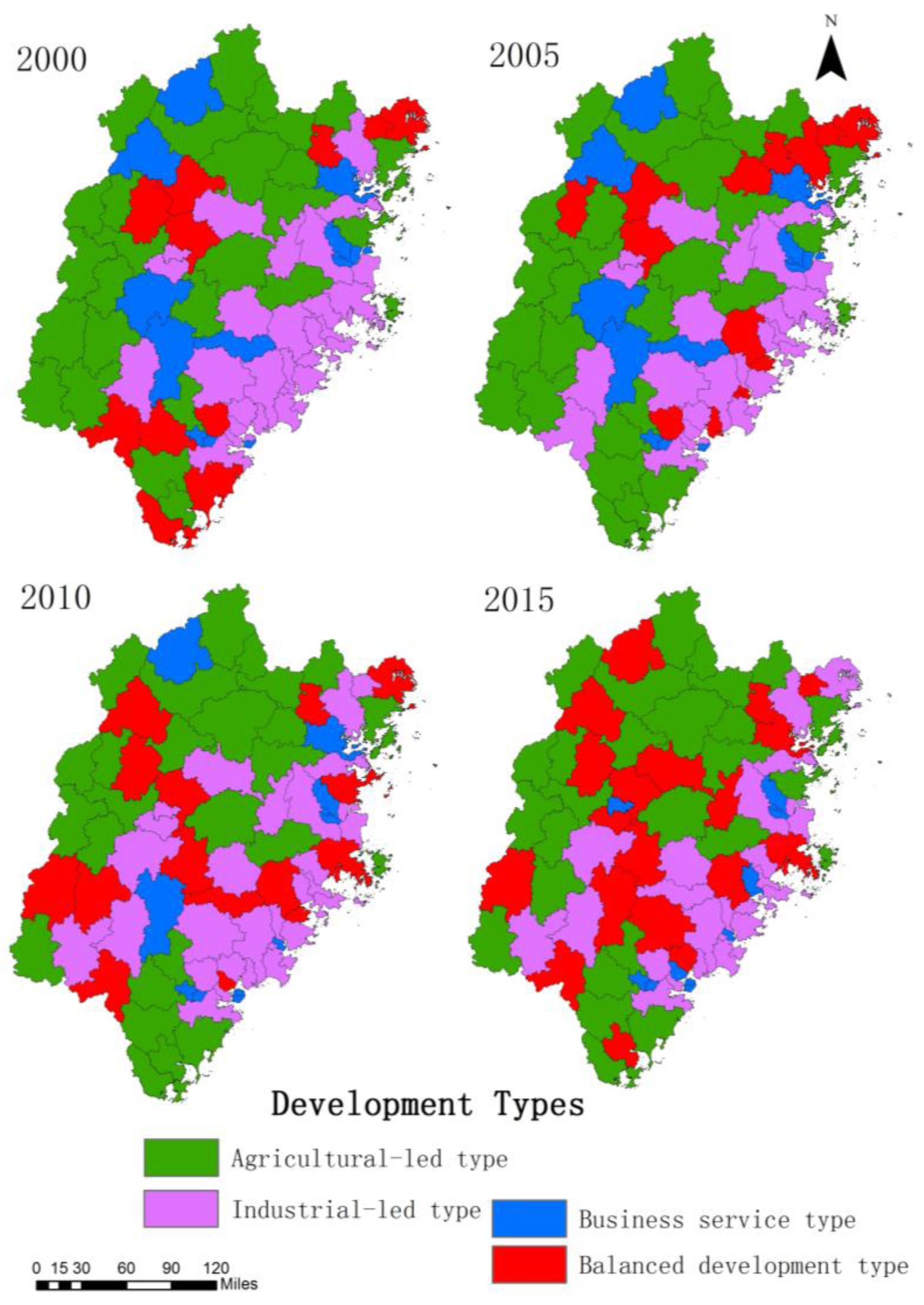
As shown in Table 5 and Figure 3, the rural development type of counties underwent changes in the period 2000–2015. Generally, the agricultural-led and industrial-led types were the foremost, followed by the business service and balanced development types. The number of agricultural-led and industrial-led counties showed fluctuating changes. The number of industrial-led counties decreased, while the balanced development areas increased significantly, with these increases mainly concentrated in the central and western regions. The number of business service type counties decreased, and this change was mainly concentrated in the central and western regions; most of the affected counties transformed into balanced development type counties (In Table 5, the agricultural-led counties in 2000 all remained agricultural-led in 2015, and the increase in the number of agricultural-led counties was due to counties moving from the balanced development category between 2000 and 2015. Three industrial-led type counties moved into the business services type category; however, three business services type counties changed to the industrial-led type and six changed to the balanced development type, so the business services type category had six (+3 -3 -6 = -6) fewer counties in 2015 than 2000. The decrease in the number of industrial-led type counties and the increase in the number of balanced development type counties occurred for similar reasons.)
As shown in Table 6, the agricultural-led counties’ rurality was at a level above “strong” and was relatively stable; most of these counties had an IRR > 0.7. There was no village below the level of “strong”. The rurality of industrial-led counties was at a level of “weak” to “very strong”; most counties had “strong” rurality, but the IRR was on a declining trend. Most of the business services-type counties were at a “very weak” or “weak” rurality level, a few were at a “strong” or “very strong” level, and the number of “very strong” rurality counties decreased from 7 to 0; the overall trend was one of declining IRR. Counties of the balanced development type were largely at a level of “strong” or “very strong”, with a few at a “weak” level.
3.2. Analysis of Coupling of Rurality and Ecosystem Services
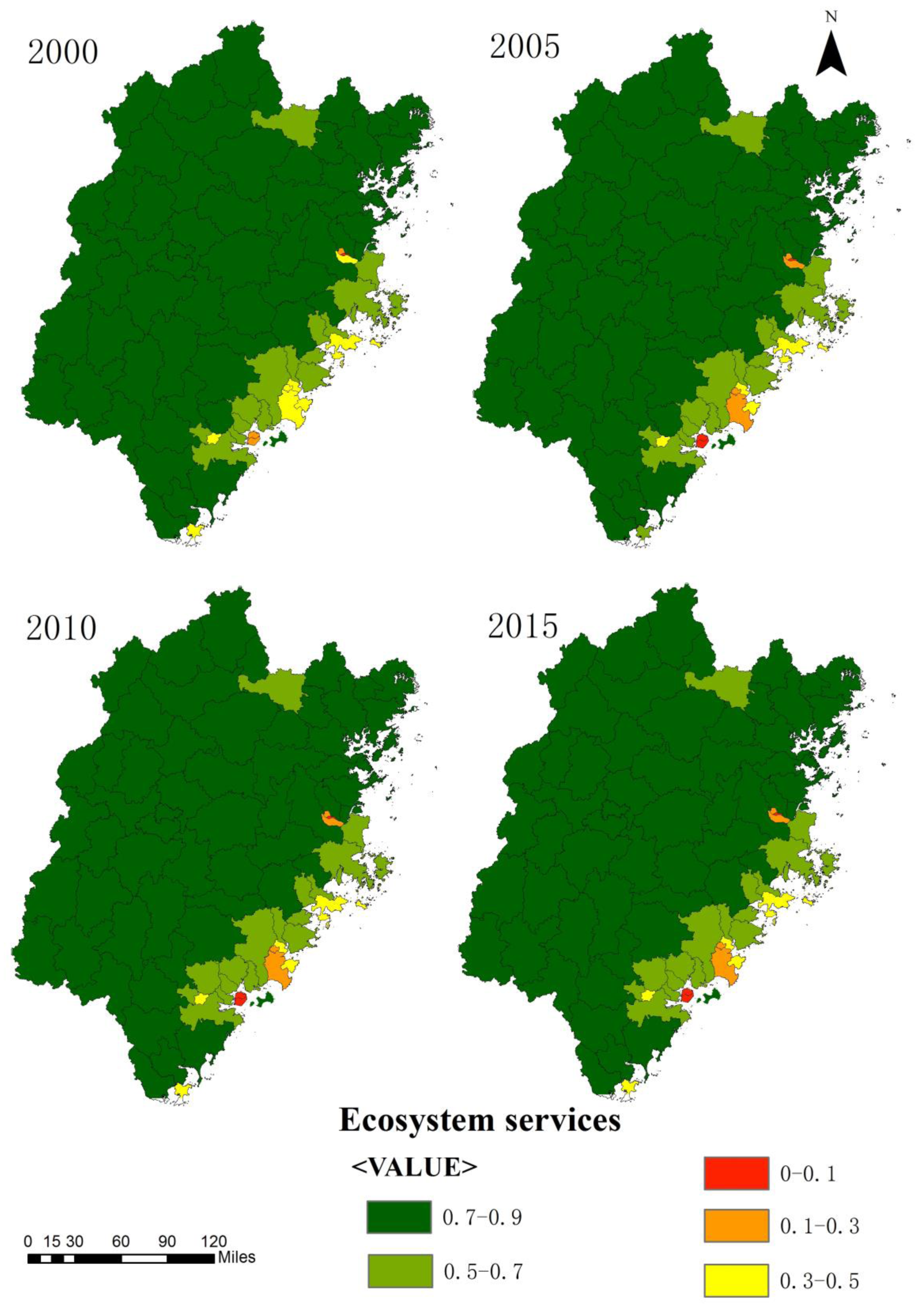
By overlaying the carbon storage, habitat quality, and water yield values, we found that the sums of the ecosystem services in eastern coastal portions of the study area were the lowest, that those in the western region were the highest, and that the sums present a pattern of gradual increase from the eastern coast to the western inland region (Figure 4). During the research period, the ecosystem services values decreased yearly, and the decreases were mainly concentrated in the southeast coast, followed by the central region.
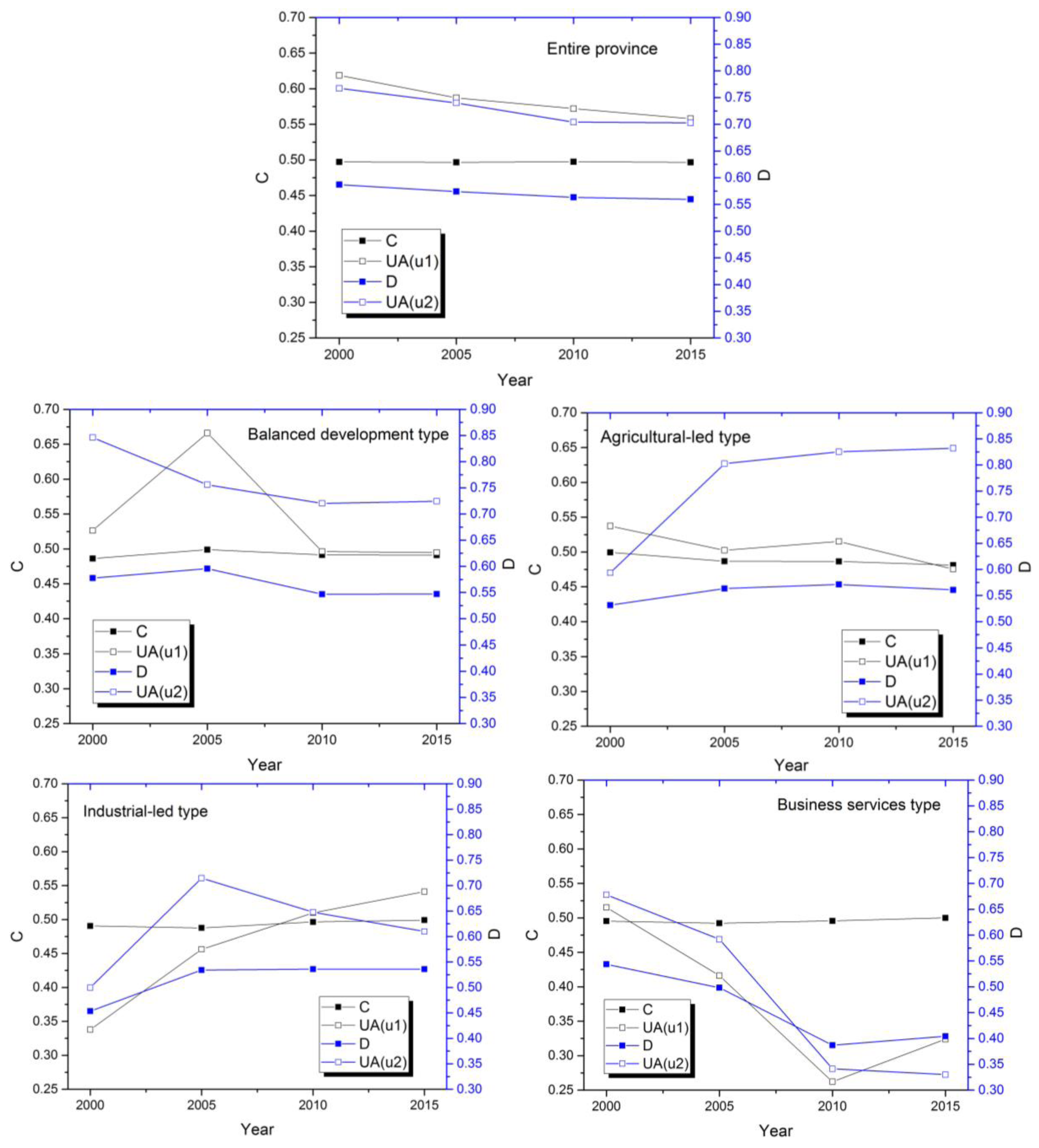
The results (Figure 5) show that the coupling coordination degrees of balanced development type, agricultural-led type and industrial-led type counties were in the high coordination stage, which shows clear synergistic between rurality and ecosystem services. This was the same as the whole province’s coupling coordination degree level. However, the business services type counties’ coupling coordination degree declined to a moderate coordination level by 2005 and to a low coordination stage by 2010, then returned to moderate coordination level again by 2015.
All the development types’ coupling degrees (Figure 5) between IRR and ES were generally near 0.5, which falls within the “antagonistic” stage but close to the “run-in” stage. This was also the same as the whole province’s coupling degree level, and it meant the system of rurality-ecosystem services had transitioned to a beneficial coupling. Although the coupling degree for the whole province decreased yearly, it still remained in a highly coordinated state.
As shown in Table 7, the correlation coefficient increased yearly during the research period (From 0.692 to 0.826 during 2000 and 2015) and all were significant at the 0.01 level. Thus, IRR was positively correlated with ES, which supports the coupling research above. The curve fitting showed that the coefficient of determination (R2) increased yearly, indicating that the degree of curve fitting and the fit of IRR to ES was better for the later years, which also supported the increasing level of coordination between rurality and ecosystem services indicated above.
In summary, the rurality of research areas weakened and the ecosystem services were reduced year by year. However, the imbalance in the distribution of rurality was alleviated and rural development gradually shifted to a balanced type during the same period. Notably, counties with agricultural and balanced development types of rural development had higher ecosystem services. The rurality and ecosystem services in industrial-led counties showed an uneven pattern: some counties had strong rurality and better ecosystem services, while others had weak rurality and poorer ecosystem services. This phenomenon was more pronounced in 2015 than that in 2000. We also observed varying levels of rurality and ecosystem services in the business services-type counties, while the rurality and ecosystem services had a relatively coordinated development pattern in the other county types.
4. Discussion
In our analysis, the rurality of counties within the research area showed a positive relationship with ecosystem services within those counties, and also some characteristics and contradictions, and the same with the coupling degree between rural development and ecosystem services. But, what were these characteristics and contradictions? What caused them and what did they mean, what impacts would they have? Are these impacts beneficial or not? How can we adjust the process of rural development to ensure that ecosystem services are maintained? We tried to analyse these questions.
4.1. Causes for Contradictions in Changes in Rural Development Types and IRR Values
According to the results of this study, the economic output and contribution of agricultural production, which was the primary sector in 2000, decreased during the research period, but the number of agricultural-led counties increased (Table 1, Table 5 and Table 6). Additionally, the economic output and contribution of tertiary industry increased but decreased in the number of business services type counties. To understand this contradiction, we analyzed the raw data and found that from 2000 to 2015 the output value of tertiary industry in a few counties increased substantially; this accounted for a large proportion of the total output value of Fujian province and raised the output and contribution rate of tertiary industry as a whole. Although the output value of secondary industry also increased, its contribution rate declined due to the increase in output value of tertiary industry in some regions. The increase in the number of balanced development type counties and the substantial increase in the output value of tertiary industry in some counties meant that the output value of both secondary and tertiary industries increased. Meanwhile, the output value of secondary and tertiary industries tended to be much larger than that of primary industry, which caused the proportion and contribution rate of primary industry to decline while the overall economic output increased.
The changes in rural development types and the decline of IRR followed similar patterns, which reflected the fact that the reductions in the rurality index were largely related to the changes in rural development types. Although the number of agricultural-led and balanced development areas increased, and these areas had higher average rurality, the overall rurality of Fujian province decreased during the research period. The reason for this phenomenon was that the decreases in rurality of industrial-led and business services-type counties outweighed the increases due to changes in rural development types, and the rurality of some agricultural-led and balanced development areas decreased (Table 6).
To a certain degree, the phenomenon of certain counties driving the overall trends (changes in rurality and ecosystem services) meant that urbanization and rural development were occurring intensely in some concentrated areas of Fujian, mainly around the capital city and the heavily developed in southeast. These changes were happening locally, those areas in which rural development and ecosystem services came into more serious conflict should receive more attention in the planning of development planning and management of development. How should decision makers regulate the trade-offs between the two? That question merits further consideration and research.
4.2. Analysis of Coupling between Rural Development and Ecosystem Services
Rural development usually relies on industry [20]. Different types of rural development may have the same or similar values on the rurality index; this is mainly due to the diversification of rural development in the current context of globalization and socio-economic reconstruction [45]. Industry, tourism, agriculture and business services have developed rapidly in some rural areas due to rapid economic development, improvements in the transportation system, and upgrades to information technology networks. This makes rurality values of some counties significantly different from those of similar regions; in other cases, the same rurality index value corresponds to different types of rural development [20]. At the same time, different types of development leave different impacts on the resources of the surrounding environment. Business services and industrial-led development consume far more resources and influence the environment to a much greater extent than does agriculture-led development [2]. Once a rural development’s use of resources is higher than the level the ecosystem can tolerate, the ecosystem services it provides will be reduced or even depleted [2]. In turn, reduced or depleted ecosystem services may inhibit further development of the village.
Our results (Figure 5) show that in many Fujian counties between 2000 and 2015, rurality and ecosystem services were in the “antagonistic” stage, but were approaching the “run-in” stage. This means that both rurality and the value of ecosystem services initially declined with the rapid development of rural areas, but ecosystem services then began to improve, likely because municipalities began to place more emphasis on ecosystem services’ protection and maintenance. The coupling coordination degree was high (with the exception of the business services type counties), and the rurality and ecosystem services were in harmony with each other during development, which reflected the tendency of this system to move from disorder to order. These results show that development in Fujian has crossed from the mode of simply pursuing economic benefits and has embarked on the path of maintaining both economy and ecology, at least to some degree. However, the gradual reduction in the coupling coordination degree we observed during the study period means that the negative impacts of social and economic activities on natural resource use and ecological environment have been increasing, especially in business services type counties (according to the study, reduction in the coupling coordination degree of the whole province was mainly due to the decline in the coupling coordination degrees of business services type counties), and that there will be dangerous if appropriate measures are not taken.
Additionally, according to 2013 research by Chen, Peng and Xiong [44], the lack of coordination of internal structure (which means the population composition, industrial structure and policy differences, etc.) of economic development hinders sustainable development since the order parameter of social economy was higher than ecological environment’s in Dongting Lake. So, they thought the ecological environment was the main bottleneck to economic development, the economic development dominated the evolution of society and the ecological environment. In our research, all of the rural development type’s order parameters (UA(U2) > UA(U1)) of ecosystem services were higher than the rurality index’s, so the lack of coordination of internal structure (which means the composition of various types of ecosystem services) of ecosystem services may be important factors affecting Fujian’s increasing decline in coupling coordination degree between rurality and ecosystem services, especially in business services type counties, too.
4.3. Implications for Policy Making
Counties with chiefly agricultural development have high ecosystem services, however, they have limitations, and the economic benefits they can produce are far less than other development types [2]. Therefore, agriculture alone is not an ideal rural development model. Similarly, the commercial services counties enjoy greater economic benefits but lower ecosystem services: only a few of these counties achieved both high economic benefits and high ecosystem services. Therefore, commercial service-led development was not the best rural development model either. While the industrial-led counties enjoyed some economic benefits, the decline of rurality year after year led to a corresponding decline in ecosystem services. Therefore, considering its comprehensive benefits for economics and ecosystems, the balanced development type was the ideal mode for the development of rural areas in Fujian. This means the well-coordinated inclusion of agriculture, industry and business services in the economic development of a county. Only this development type is likely to provide high economic efficiency coexisting with higher rurality.
However, the balanced development type is likely not an ideal fit for all counties. Counties should plan for development according to local conditions. Agricultural-led areas should rely on local resources, strengthen infrastructure to modernize agricultural production, preserve and improve beautiful rural landscapes and towns, and promote the development of rural tourism and other green industry. Industrial-led areas should promote green development and give full play to the industrial cluster effect (In 2000, Hill and Brennan [46,47] defined an industrial cluster as a system that enables component firms and institutes to generate higher unit earnings and more efficient operations owing to innovations stimulated by intense geographic concentration). Business services-type counties should strengthen the protection of the environment while creating a unique brand and enhancing their industrial vitality and competitiveness [21]. In general, it is our view that regions that benefit from a strong economy and high ecosystem services should continue to maintain both, and those with a poor economy and lower ecosystem services should give priority to economic development while working to improve their ecosystem services appropriately. Industrial-led and business services type counties that have a good economy but low ecosystem services should also aim to protect and support local ecosystems.
Currently, significant funding has been invested in project like green industries and rural tourism to reduce damage to ecosystem services in order to pursue both economic and ecological benefits in Fujian. And the increase in balanced development-type counties also shows the implementation of “beautiful villages” programs [48] has achieved economic and ecological benefits. The development in these rural areas has not depended solely on agriculture, but instead has balanced agriculture, industry and business services. This is in line with current trends encouraging green, healthy and sustainable development globally [49]. However, there is still a long way to go. Agriculture and industry still play an important role in economic development, and rural development’s consumption of resources caused decreases in ecosystem services in the study area year by year. Therefore, it is necessary to make tradeoffs between economic and ecological benefits, different ecosystem services and industries. Further research into these issues is warranted.
4.4. Innovation and Limitation
The innovation of this article lies in the combined analysis of rurality and ecosystem services. As urbanization progresses, the development of rural areas will inevitably bring changes to ecosystem services. The methods used in this study can be employed to analyze regional development in the past and present, investigate whether current development modes have a positive or negative impact on ecosystem services, and explore whether this is beneficial to regional sustainable development and what can be improved. The methods presented in this article were relatively reasonable with no specific parameters and are applicable both to other provinces of China and to other countries.
Certainly, rurality cannot be expressed simply though a few indicators; IRR is a relative value [50]. In this paper, the indicators in the relative rurality index calculation do not fully reflect all characteristics of regional rurality. Therefore, future research should focus on the selection of rural indicators to give full consideration to other aspects of rurality. Ecosystem services include supporting services, provisioning services, regulating services, and cultural services. Our research lacks a cultural service component, and our choices of carbon storage, habitat quality and water yield to represent supporting, provisioning and regulating ecosystem services were somewhat subjective. Therefore, this paper should not be considered a comprehensive analysis of rurality and ecosystem services. However, our results will assist in efforts to promote economic development while maintaining ecosystem services, and will provide theoretical and decision-making support for coordination between rural development and ecosystem services in China and worldwide.
5. Conclusions
Taking Fujian province of China as the study area for this case study, we analyzed the coupling between rural development and ecosystem services. We found that rurality and ecosystem services are related to each other and that rural development and ecosystem services were often in harmony, but that social and economic activities sometimes produced negative impacts on the environment as development increased. Changes and trade-offs between rural development and ecosystem services in Fujian occurred locally and were intense in more economically developed areas. Unbalanced development occurred in some counties. The results presented in this article supplement previous studies on rural development and ecosystem services in China and could aid in rural planning and management. At the same time, these results could be used as a basis for further studies exploring conflicts between rural development and the environment, trade-offs and synergies among different ecosystem services, and the impact of sustainable development on social, natural, ecological and economic activity.
Acknowledgments
This work was supported by the National Key R&D Program of China (2016YFC0502902) and the National Natural Science Foundation of China (41501196 and 41471137).
Author Contributions
Lina Tang, Quanyi Qiu, Su Xu mainly contributed by making valuable comments and suggestions on the writing and revision of the paper. Lishan Xiao mainly contributed by studying and summarizing the calculation method for the Relative Rurality Index. Tong Wu and Ziyan Wang participated in data collection and processing. All authors have read and approved this manuscript.
Conflicts of Interest
The authors declare no conflict of interest.
References
- Meng, L.; Huang, J.; Dong, J. Assessment of rural ecosystem health and type classification in Jiangsu province, China. Sci. Total Environ. 2018, 615, 1218–1228. [Google Scholar] [CrossRef]
- Millenium Ecosystem Assessment (MA). Ecosystems and Human Well-being: General Synthesis. Available online: http://www.millenniumassessment.org/documents/document.356.aspx.pdf (accessed on 1 November 2017).
- Ding, B.; Li, X.M.; Sun, X.H.; Wang, R.Q.; Zhang, S.P. Impacts of economic development models on ecosystem service values: A case study of three mountain villages in Middle Shandong, China. Acta Ecol. Sin. 2016, 36, 3042–3052. [Google Scholar] [CrossRef]
- Zhang, F.; Liu, Y. Dynamic Mechanism and Models of Regional Rural Development in China. Acta Geogr. Sin. 2008, 63, 115–122. [Google Scholar]
- Zheng, H.; Ouyang, Z.; Zhao, T.; Xu, W. The impact of human activities on ecosystem services. J. Nat. Resour. 2003, 18, 118–126. [Google Scholar]
- Ouyang, Z.; Wang, R.; Zhao, J. Ecosystem services function and evaluation about it’s eco-economic value. Chin. J. appl. Ecosyst. Ecol. 1999, 10, 635–640. [Google Scholar]
- Zhang, X. On discriminnation of rural definitions. Acta Geogr. Sin. 1998, 79–85. [Google Scholar] [CrossRef]
- Long, H. Land use transition and rural transformation development. Prog. Geogr. 2012, 31, 131–138. [Google Scholar]
- Bai, Y.; Zheng, H.; Zhuang, C.; Ouyang, Z. Ecosystem services evaluation and its regulation in Baiyangdian basin. Acta Ecol. Sin. 2013, 33, 711–717. [Google Scholar]
- Vitousek, P.M.; Mooney, H.A.; Lubchenco, J. Human domination of Earth’s ecosystems. Science 1997, 277, 494–499. [Google Scholar] [CrossRef]
- Costanza, R.; Mageau, M. What is a healthy ecosystem? Aquat. Ecol. 1999, 33, 105–115. [Google Scholar] [CrossRef]
- Woods, M. Engaging the global countryside: Globalization, hybridity and the reconstitution of rural place. Prog. Hum. Geogr. 2007, 31, 485–507. [Google Scholar] [CrossRef]
- Cai, Y.; Lu, D.; Zhou, Y.; Wang, J.; Qin, Q.; Li, Y.; Chai, Y.; Zhang, Y.; Liu, W.; Wang, J.; et al. Chinese progress and international trends of geography. Acta Geogr. Sin. 2004, 59, 803–810. [Google Scholar]
- Norton, L.; Greene, S.; Scholefield, P.; Dunbar, M. The importance of scale in the development of ecosystem service indicators. Ecol. Indic. 2016, 61, 130–140. [Google Scholar] [CrossRef]
- Woods, M. Advocating rurality? The repositioning of rural local government. J. Rural Stud. 1998, 14, 13–26. [Google Scholar] [CrossRef]
- Woods, M. Performing rurality and practising rural geography. Prog. Hum. Geogr. 2010, 34, 835–846. [Google Scholar] [CrossRef]
- Cloke, P. An index of rurality for England and Wales. Reg. Stud. 1977, 11, 31–46. [Google Scholar] [CrossRef]
- Cloke, P.; Edwards, G. Rurality in England and Wales 1981: A replication of the 1971 index. Reg. Stud. 1986, 20, 289–306. [Google Scholar] [CrossRef]
- Waldorf, B.S. A Continuous Multi-Dimensional Measure of Rurality: Moving Beyond Threshold Measures; Annual Meeting of American Agricultural Economic Association: Long Island, CA, USA, 2006. [Google Scholar]
- Long, H.; Liu, Y.; Zou, J. Assessment of rural development types and their rurality in eastern coastal China. Acta Geogr. Sin. 2009, 64, 426–434. [Google Scholar]
- Liang, Z.; Feng, Y. Rural development types and the Spatio-temporal changes of rurality in Guangdong Province. Trop. Geogr. 2016, 36, 995–1004. [Google Scholar]
- Li, B.; Chen, D.; Wu, S.; Zhou, S.; Wang, T.; Chen, H. Spatio-temporal assessment of urbanization impacts on ecosystem services: Case study of Nanjing City, China. Ecol. Indic. 2016, 71, 416–427. [Google Scholar] [CrossRef]
- BenDor, T.K.; Spurlock, D.; Woodruff, S.C.; Olander, L. A research agenda for ecosystem services in American environmental and land use planning. Cities 2017, 60, 260–271. [Google Scholar] [CrossRef]
- Zhou, H. The Modern Chinese Dictionary; Guangming Daily Press: Beijing, China, 2003; pp. 820–821. [Google Scholar]
- Li, Y.; Li, Y.; Zhou, Y.; Shi, Y.; Zhu, X. Investigation of a coupling model of coordination between urbanization and the environment. J. Environ. Manag. 2012, 98, 127–133. [Google Scholar] [CrossRef] [PubMed]
- Xiong, J.; Chen, D.; Peng, B.; Deng, S.; Xie, X. Spatio-temporal difference of coupling coordinative degree of ecological carrying capacity in the Dongting Lake region. Prog. Geogr. 2014, 34, 1108–1116. [Google Scholar]
- Wu, Y.; Zhang, Y.; Wang, Q.; Lang, D. On environment-economy coordinated degree. Environ. Pollut. Control 2001, 25–29. [Google Scholar]
- Liu, Y.; Song, X. Coupling Degree Model and Its Forecasting Model of Urbanization and Ecological Environment. J. China Univ. Min. Technol. 2005, 34, 91–96. [Google Scholar]
- Salvati, L.; Carlucci, M. The economic and environmental performances of rural districts in Italy: Are competitiveness and sustainability compatible targets? Ecol. Econ. 2011, 70, 2446–2453. [Google Scholar] [CrossRef]
- Pfeifer, C.; Sonneveld, M.P.W.; Stoorvogel, J.J. Farmers’ contribution to landscape services in the Netherlands under different rural development Scenarios. J. Environ. Manag. 2012, 111, 96–105. [Google Scholar] [CrossRef] [PubMed]
- Fujian Statistical Yearbook. Available online: http://www.stats-fj.gov.cn/xxgk/ndsj/ (accessed on 1 November 2016).
- Resources and Environment Science Data Center, Chinese Academy of Sciences. Available online: http://www.resdc.cn/Datalist1.aspx?FieldTyepID=1,3 (accessed on 1 November 2016).
- China Meteorological Data Network. Available online: http://data.cma.cn/data/index/6d1b5efbdcbf9a58.html (accessed on 1 November 2016).
- Xiao, L.; Yu, Z.; Ye, H.; Guo, Q. The research of coupling rural development and economy cluster in Fujian province. Acta Geogr. Sin. 2015, 70, 615–624. [Google Scholar]
- Li, X.; Li, Z.; Weng, C.; Wang, S. Assessing the county’s rural development types and their rurality: A case study of the Three Gorges Eco-Economic region in Chongqing. J. Chongqing Norm. Univ. (Nat. Sci. Ed.) 2013, 1, 42–47. [Google Scholar]
- Zhang, R.; Jiao, H.; Zhang, X. Rural development types and rurality in the Yangtze River Delta. J. Nanjing Norm. Univ. (Eng. Technol. Ed.) 2014, 37, 132–136. [Google Scholar]
- Natural Capital Project. Available online: www.naturalcapitalproject.org (accessed on 1 May 2017).
- Wu, D.; Li, C. Chen, L. Principles and Application of Synergetics; Huazhong University of Science and Technology Press: Wuhan, China, 1990; pp. 9–17. [Google Scholar]
- Zeng, Z.X. The analysis of coordination and sustainable development. Syst. Eng. Theory Pract. 2001, 3, 18–21. [Google Scholar]
- Meng, Q.S.; Han, W.X.; Jin, R. Study of coordinating model for the co-system of science and technology and economy. J. Tianjin Norm. Univ. (Nat. Sci. Ed.) 1998, 18, 8–12. [Google Scholar]
- Vefie, L. The Penguin Directionary of Physics; Foreign Language Press: Beijing, China, 1996; pp. 92–93. [Google Scholar]
- Liu, D.; Yang, Y. Coupling coordinative degree of regional economy- tourism- ecological environment: A case study of Anhui province. Resour. Environ. Yangtze Basin 2011, 20, 892–896. [Google Scholar]
- Ma, L.; Jin, F.; Liu, Y. Spatial Pattern and Industrial Sector Structure Analysis on the Coupling and Coordinating Degree of Regional Economic Development and Environmental Pollution in China. Acta Geogr. Sin. 2012, 67, 1299–1307. [Google Scholar]
- Tang, Y.; Zhu, W.; Zhang, H.; Song, Y. A review on principle and application of the InVEST model. Ecol. Sci. 2015, 34, 204–208. [Google Scholar]
- Chen, D.; Peng, B.; Xiong, J. The coupling characteristics of Eco-economic system in Dongting Lake Area. Prog. Geogr. 2013, 33, 1338–1346. [Google Scholar]
- Hill, E.W.; Brennan, J.F. A methodology for identifying the drivers of industrial clusters: The foundation of regional competitive advantage. Econ. Dev. Q. 2000, 14, 65–96. [Google Scholar] [CrossRef]
- Lin, C.; Tung, C.; Huang, C. Elucidating the industrial cluster effect from a system dynamics perspective. Technovation 2006, 26, 473–482. [Google Scholar] [CrossRef]
- Opinions of Fujian Provincial People’s Government on Further Improving the Living Environment in Rural Areas and Promoting the Beautiful Country Construction. Available online: http://www.fujian.gov.cn/zc/zxwj/szfwj/201412/t20141204_898642.htm (accessed on 1 November 2017).
- Giddings, B.; Hopwood, B.; Brien, G.O. Environment, economy and society: Fitting them together into sustainable development. Sustain. Dev. 2002, 10, 187–196. [Google Scholar] [CrossRef]
- Qi, M.; He, W. Rural development type in Jiangsu coastal areas and its rurality evaluation. Rural Econ. Sci. Technol. 2016, 27, 210–213. [Google Scholar]
Figure 1.
Map of Fujian Province, its population (2015) and it’s location in China (inset).

Figure 2.
Spatial distribution of relative rurality index in various years.
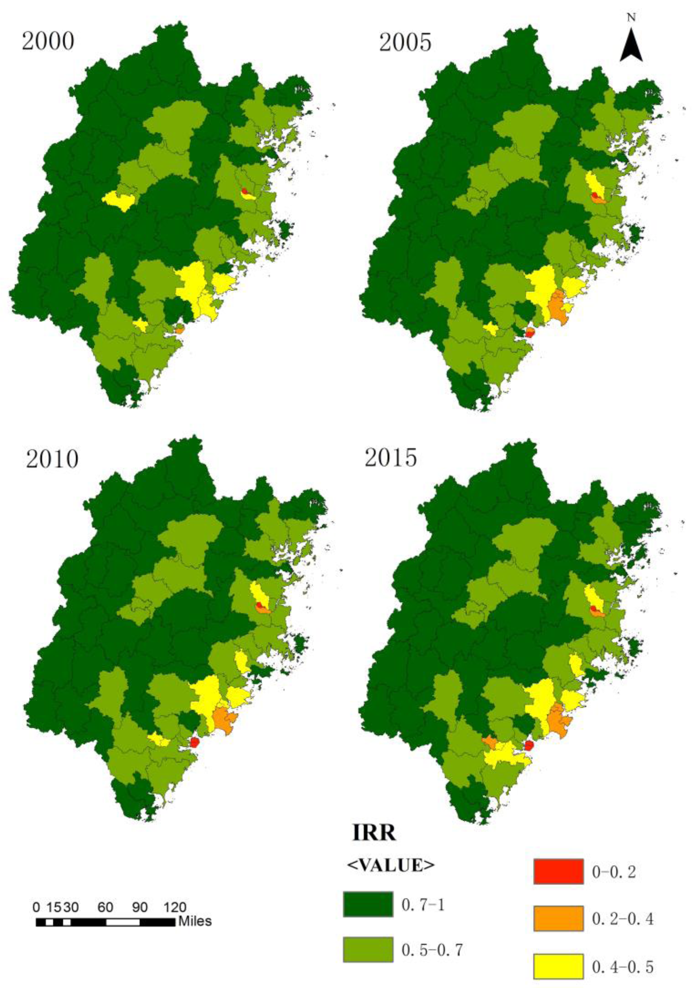
Figure 3.
Spatial distribution of rural development types in various years.

Figure 4.
Spatial distribution of ecosystem service in various years.

Figure 5.
Coupling and coupling coordinative degree between relative rurality index and ecosystem services. Notes: C is the coupling degree, D is the coupling coordination degree, UA(u1) is the comprehensive sequence parameter of the rurality index, UA(u2) is the order parameter of ecosystem services.


Table 1.
Population and economic output of Fujian 2000–2015.
| Population (Million) | Regional GDP (Billion Yuan) | Primary Industry | Secondary Industry | Tertiary Industry | ||||
|---|---|---|---|---|---|---|---|---|
| The Output (Billion Yuan) | Contribution Rate (%) | The Output (Billion Yuan) | Contribution Rate (%) | The Output (Billion Yuan) | Contribution Rate (%) | |||
| 2000 | 34.10 | 376.45 | 64.06 | 4.7 | 162.85 | 59.6 | 149.55 | 35.7 |
| 2005 | 35.57 | 655.47 | 85.54 | 3.0 | 318.89 | 51.3 | 251.11 | 45.7 |
| 2010 | 36.93 | 1473.71 | 136.37 | 2.1 | 752.28 | 67.9 | 585.06 | 30.0 |
| 2015 | 38.39 | 2597.98 | 211.81 | 2.9 | 1306.48 | 46.6 | 1079.69 | 50.5 |
Table 2.
Classification of index of relative rurality (IRR) values.
| Very Weak | Weak | Moderate | Strong | Very Strong | |
|---|---|---|---|---|---|
| Intervals of the value | [0.00, 0.20) | [0.20, 0.40) | [0.40, 0.50) | [0.50, 0.70) | [0.70, 1.00] |
Table 3.
Standards and proportions of rural development types in various years.
| Type | 2000 | 2005 | 2010 | 2015 |
|---|---|---|---|---|
| Agricultural-led | GDP1 ≥ 32.92% | GDP1 ≥ 30.00% | GDP1 ≥ 22.49% | GDP1 ≥ 18.75% |
| Industrial-led | GDP2 ≥ 44.06% | GDP2 ≥ 47.26% | GDP2 ≥ 52.78% | GDP2 ≥ 55.37% |
| Business services | GDP3 ≥ 37.86% | GDP3 ≥ 40.08% | GDP3 ≥ 42.30% | GDP3 ≥ 42.95% |
| Balanced development | Not belong to three scenarios above | Not belong to three scenarios above | Not belong to three scenarios above | Not belong to three scenarios above |
Notes: GDP1 refers to the proportion of the primary industry’s GDP in the whole regional GDP; GDP2 refers to the proportion of the secondary industry’s GDP in the whole regional GDP; GDP3 refers to the proportion of the tertiary industry’s GDP in the whole regional GDP.
Table 4.
Statistics of relative rurality index in various years.
| Max | Min | Average | SD | Skewness | Kurtosis | |
|---|---|---|---|---|---|---|
| 2000 | 0.9568 | 0.1460 | 0.6773 | 0.1578 | −0.9391 | 1.4814 |
| 2005 | 0.9649 | 0.1223 | 0.6609 | 0.1814 | −0.9938 | 0.9849 |
| 2010 | 0.9657 | 0.1245 | 0.6601 | 0.1885 | −0.9612 | 0.8325 |
| 2015 | 0.9687 | 0.1232 | 0.6597 | 0.1959 | −0.9908 | 0.7099 |
Table 5.
Changes in the rural development types of counties between 2000 and 2015.
| Year | 2015 | ||||
|---|---|---|---|---|---|
| Types | Agricultural-Led | Industrial-Led | Business Services | Balanced Development | |
| 2000 | Agricultural-led | ||||
| Industrial-led | 3 | 5 | |||
| Business services | 3 | 6 | |||
| Balanced development | 4 | ||||
| Changes in number (2015 than 2000) | 4 | −5 | −6 | 7 | |
Table 6.
Number of counties by relative rurality index and rural development type.
| Year | Interval of Rurality Index | Total Number of Counties | Change Over Past 5 Years | Types | ||||
|---|---|---|---|---|---|---|---|---|
| 0–0.2 | 0.2–0.4 | 0.4–0.5 | 0.5–0.7 | 0.7–1 | ||||
| 2000 | 3 | 21 | 24 | Agricultural-Led Type | ||||
| 2005 | 6 | 24 | 30 | 6 | ||||
| 2010 | 5 | 22 | 27 | −3 | ||||
| 2015 | 5 | 23 | 28 | 1 | ||||
| Changes over 15 years | 2 | 2 | 4 | |||||
| 2000 | 5 | 17 | 8 | 30 | Industrial-Led Type | |||
| 2005 | 2 | 3 | 14 | 7 | 26 | −4 | ||
| 2010 | 2 | 4 | 16 | 8 | 30 | 4 | ||
| 2015 | 3 | 3 | 12 | 7 | 25 | −5 | ||
| Changes over 15 years | 3 | −2 | −5 | −1 | −5 | |||
| 2000 | 2 | 1 | 2 | 6 | 7 | 18 | Business Services Type | |
| 2005 | 3 | 1 | 2 | 3 | 5 | 14 | −4 | |
| 2010 | 4 | 1 | 4 | 1 | 2 | 12 | −2 | |
| 2015 | 4 | 3 | 3 | 2 | 12 | |||
| Changes over 15 years | 2 | 2 | 1 | −4 | −7 | −6 | ||
| 2000 | 4 | 8 | 12 | Balanced Development Type | ||||
| 2005 | 2 | 6 | 6 | 14 | 2 | |||
| 2010 | 6 | 9 | 15 | 1 | ||||
| 2015 | 7 | 12 | 19 | 4 | ||||
| Changes over 15 years | 3 | 4 | 7 | |||||
Table 7.
Correlation analysis between relative rurality index and ecosystem services.
| Correlation Coefficient (R) | Multiple Correlation Coefficient | Coefficient of Determination (R2) | |
|---|---|---|---|
| 2000 | 0.692 | 0.829 | 0.687 |
| 2005 | 0.796 | 0.849 | 0.722 |
| 2010 | 0.808 | 0.887 | 0.787 |
| 2015 | 0.826 | 0.899 | 0.809 |
© 2018 by the authors. Licensee MDPI, Basel, Switzerland. This article is an open access article distributed under the terms and conditions of the Creative Commons Attribution (CC BY) license (http://creativecommons.org/licenses/by/4.0/).
Share and Cite
MDPI and ACS Style
Chen, H.; Tang, L.; Qiu, Q.; Wu, T.; Wang, Z.; Xu, S.; Xiao, L. Coupling between Rural Development and Ecosystem Services, the Case of Fujian Province, China. Sustainability 2018, 10, 524. https://doi.org/10.3390/su10020524
AMA Style
Chen H, Tang L, Qiu Q, Wu T, Wang Z, Xu S, Xiao L. Coupling between Rural Development and Ecosystem Services, the Case of Fujian Province, China. Sustainability. 2018; 10(2):524. https://doi.org/10.3390/su10020524
Chicago/Turabian StyleChen, Huaxiang, Lina Tang, Quanyi Qiu, Tong Wu, Ziyan Wang, Su Xu, and Lishan Xiao. 2018. "Coupling between Rural Development and Ecosystem Services, the Case of Fujian Province, China" Sustainability 10, no. 2: 524. https://doi.org/10.3390/su10020524
Note that from the first issue of 2016, this journal uses article numbers instead of page numbers. See further details here.