Application of Bayesian Multilevel Models Using Small and Medium Size City in China: The Case of Changchun


1
MOE Key Laboratory for Urban Transportation Complex Systems Theory and Technology, Beijing Jiaotong University, Beijing 100044, China
2
Key Laboratory of Transport Industry of Big Data Application Technologies for Comprehensive Transport, Beijing Jiaotong University, Beijing 100044, China
3
Department of Geography, University of Cambridge, Downing Place, Cambridge CB2 3EN, UK
*
Author to whom correspondence should be addressed.
Sustainability 2018, 10(2), 484; https://doi.org/10.3390/su10020484
Submission received: 29 December 2017
/
Revised: 4 February 2018
/
Accepted: 8 February 2018
/
Published: 11 February 2018
Abstract
:Concerns about transportation energy consumption and emissions force urban planners and policy makers to pay more attention to the effects of car ownership and use on the environment in China. However, few studies have investigated the relationship between the built environment and car ownership and use in China, especially in mid-sized and small cities. This study uses Changchun, China as a case study and examines the potential impacts of the built environment and socio-demographics on car ownership and use for commuting simultaneously using Bayesian multilevel binary logistic models. Furthermore, the spatial autocorrelation of car ownership and use is recognized across traffic analysis zones (TAZs), which are specifically represented by the conditional autoregressive (CAR) model. The estimated results indicate that socio-demographic characteristics have significant effects on car ownership and use. Moreover, the built environment measured at the TAZ level still shows a significant association with other factors controlled. Specifically, it suggests that denser residential density, compact land use, better transit services and street connectivity can reduce car dependency more effectively. This study provides new insights into how the built environment influences the car ownership and use, which can be useful for urban planners and policy makers to develop strategies for reducing car dependency.
1. Introduction
In recent years, the number of cars has increased rapidly due to rapid urbanization, rising incomes, and demand for motorized travel, especially in developing countries [1,2]. Car ownership per 1000 people increased to 77 in 2013, which is almost 100 times what it was in 1990 in mainland China [3]. An explosive growth of car ownership and use has also brought a series of problems, such as traffic congestion, energy consumption and air pollution [4,5], which attracts more attention from the government and policy makers in China [6]. Therefore, studies on the determiners and how they influence the car ownership and use have gained wide interests among transportation researchers [7,8,9,10]. To address the challenges, it is widely acknowledged that a solution to reduce car dependency by promoting urban development patterns [11,12,13,14,15,16,17,18,19,20], in which built environment plays an important role [21]. Moreover, the built environment could change with rapid urbanization in China, which also provides a good opportunity for understanding the link between the built environment and car dependency.
The impacts of the built environment on car ownership and use have gained more and more attention due to its contribution to traffic congestion and environmental issues in developed countries [22,23,24]. However, there are several major gaps that need to be filled. First, although many studies have explored these impacts in developed countries, little is known about the relationship in urban China, especially in the context of small or mid-sized cities, in which car ownership and use is still increasing rapidly [21,25]. With rapid urbanization, many Chinese cities are reshaping their spatial forms and the number of car ownership is still growing constantly, which is significantly different from western cities. In addition, a few Chinese cities are planning to build transit cities and invest huge amounts of capital in developing public transit as a way to reduce car dependency. These characteristics may show that findings in developed countries are not transferable to cities in China. Second, few prior studies exploring the impacts of the built environment on car dependency take into account spatial autocorrelation, which might lead to misunderstanding the role the built environment plays. The spatial autocorrelation, which has been studied in spatial economics by several approaches and proven to create an effect on travel behavior [26,27,28], is still rarely considered in existing studies.
The paper aims to fill the aforementioned gaps and examine the influences of built environment on car ownership and use in a rapidly developing country using the household travel survey data in Changchun, China. Additionally, Bayesian multilevel binary logistic models incorporating spatial autocorrelation are employed to investigate the influences.
This paper is organized as follows. The following section presents the related research. The third section gives the data and model variables. The fourth section describes Bayesian multilevel binary logistic models. The fifth section presents the results. The final section summarizes the important findings and recommendations.
2. Literature Review
Built environment characteristics are summarized as the “D variables” including density, design, diversity, destination accessibility and distance to transit [29,30,31,32,33]. A few studies have investigated the influence of the built environment on car dependency as problems related to driving gained more attention [6]. However, previous studies have returned some debatable conclusions about the influences [13]. For example, some researchers believe that improving the built environment can reduce car use and help reduce traffic congestion [34]. However, others doubt the conclusion and hold the view that the influence is not direct and the travel distance become longer as the built environment is improved [35].
2.1. The Impacts of Built Environment on Car Ownership and Use
Land use mixture is an important index representing land use diversity. The influences of land use diversity on car ownership have been explored the most. Most researchers claim that increasing land use mix can reduce car ownership and VMT to some extent [36,37]. However, some studies indicate that the effects of land use mix on car use are not significant [38].
Density, including residence density and employment density, is another key component that is significantly associated with car dependency. Cervero et al. [12] employed a logit model to examine the influence of density and land use mix. The results indicate that both density and land use mix have significant influences on travel behavior. Ding et al. [17] investigated the impacts of the built environment on car ownership and travel distance. The results prove that employment density has a significant influence on car ownership and travel distance, whereas the influence of residence density is only significant for car ownership.
Design is an element usually quantified by street network connection, intersection density or block size. Hong et al. [39] implemented a Bayesian model to represent the built environment’s influences on VMT, which indicated that the intersection density has an obvious effect on non-work related VMT while having not effect on work-related VMT. However, the density of the road network is used to represent design, whose results show that it is not significantly associated with car ownership [10].
Destination accessibility is a component representing a location’s characteristics, which is important for travel including travel cost and time. And it is usually quantified by distance to the central business district (CBD). Many researchers confirm that the location of residence has a significant influence on VMT and the influence is always negative [40,41,42].
Due to the explosive construction of metro and the plan to create transit cities in China, the distance to transit is playing a more important role in influencing car ownership and use. Wu et al. [2] investigated how metro construction affected car travel using Beijing as a case. The authors compared the commuting travel by car in 2005 and 2009 during which, the metro underwent explosive construction. Li et al. [32] employed a regression model to explore the influence of the built environment in neighborhoods near metro stations on car ownership and use, in which distance to the metro station was found to be a significant factor.
However, concerns about the link between the built environment and car dependency are still few in Chinese cities [10]. The built environment changes quickly with rapid urbanization, which could provide additional insights into the link.
2.2. Other Factors Influencing Car Ownership and Use
Apart from the aforementioned variables, there are also other factors influencing car ownership including socioeconomic and individual factors, household structure, trip-related information, and the traveler’s self-selection. Some of these factors are believed to be even more important than the built environment [43,44,45,46,47].
The influences of socioeconomic and individual factors on car ownership and use are well explored in many studies [48]. Income is found to be a determinant for car ownership and use both for work and non-work purposes, which also may be one of the most important factors [49,50]. Yet some researchers claim that the relationship between income and VMT is not significant [38]. The household structure including household size and the ages of children is a factor that can influence the car dependency [51,52]. Furthermore, trip-related information is another factor that was found to have a significant influence on car use. For example, Ding et al. [23] confirmed that travel cost and time had a significant influence on mode choice after controlling for the built environment and socio-demographic characteristics.
Individual attitudes and preferences which are also called self-selection effects have influence on car ownership and travel mode choice [53]. The self-selection effects represent the preferences of residents to choose their residential locations in transit-oriented neighborhoods. It has been found that self-selection can affect car ownership and commuting distance [46]. Additionally, the influence of attitudes on VMT is investigated at different geographical scales [39].
2.3. Spatial Effects in City Context
The spatial effects mainly include spatial heterogeneity and spatial autocorrelation, which were often neglected in previous studies. The multilevel model is found to be an effective way to represent spatial heterogeneity. For example, Ding et al. built a multilevel model to explore the relationship between the built environment and work-related VMT and claimed that the increasing distance from CBD generated more VMT. After the spatial heterogeneity is taken into consideration, the model performs better than the simple models [24]. However, the spatial relationship between groups cannot be captured with a multilevel model, which is also viewed as a way to display the effect of location [28]. Hong et al. [39] proposed a unified analytical framework to examine the spatial effects when exploring the influences of the built environment on VMT and found that the model considering spatial effects fit the data better. A case in Beijing considered the spatial effects and confirmed that the metro infrastructure is helpful for reducing car dependency [2]. However, spatial autocorrelation, usually considered in geographic and economic analysis, occurs when observations at nearby locations tend to have similar characteristics. Therefore, the assumption of independence of observations is no longer met. Xu et al. [54] explored the impacts of urban rail transit on commercial property value in which spatial autoregressive models were used to estimate commercial value capture. The spatial autocorrelation is also proven to exist in accidents that happen on suburban highways [55]. Moreover, the relationship between transport emissions and land use is estimated and the CAR model is found to be effective in representing the spatial autocorrelation [27]. Most statistical models ignoring the spatial autocorrelation could lead to misunderstanding the role played by the built environment in car ownership and use. However, the spatial autocorrelation is usually neglected in modeling car ownership and use.
2.4. Determinants of Car Ownership and Use in China
With the rapid development of the economy, the rate of car ownership has grown significantly in China over the past decades. It is widely believed that income is one of the most important factors influencing the car ownership and use [56]. Besides the growth of income, other socio-demographic characteristics including gender, age, education, and household structure have been found to have significant influences on car ownership and use in China [57,58,59]. In addition, there are some factors that should be taken into consideration to differentiate China from other developed countries, especially in small and mid-sized cities in China, such as the Hukou and housing sources [21]. Hukou is a special system to control the population movement from rural area to cities [60]. It is believed that Hukou system is an important factor preventing people from a few social benefits. Especially in small and mid-size cities in China, residents without local Hukou are less likely to buy a car. In addition, another factor that differentiates China from western countries is the housing source [61]. In China, the housing source is a factor influencing travel behavior. Residents living in Danwei housing are found to significantly generate shorter commuting distance either by public transport or car than those with other housing sources [32].
The built environment also plays an important role in influencing car ownership and travel in Chinese cities. For example, a case study implemented in Shanghai shows that road length per capita and intersection density in residential neighborhoods have negative impacts on car travel while the distance to CBD has significantly positive impacts. This is similar to that of western cities [62]. Jiang et al. [10] confirmed that higher land use mix generated more household VKT, but was unrelated with car ownership rates in Jinan. Liu et al. [63] employed a structure equal model to examine the relationship between the built environment and car use, which confirmed that compact land use played an important role in reducing car commuting.
Rapid urbanization brought a few problems that need to be solved urgently in China. For example, many people living in suburban areas have to work downtown where most employment opportunities concentrate, but the public transit service is lagging [32]. Many studies claim the residents living in the suburbs generate more travel time by car [64]. There are two reasons accounting for it. One is that the construction of infrastructure is hysteresis and transit service is far from satisfactory in suburbs. The other is that residents have to drive to work because most employment opportunities concentrate in the downtown.
The Chinese government has been committed to reducing the number of private cars so as to relieve traffic pressure and reduce environmental pollution. The Chinese government is constructing metro stations in many cities and planning to create a few transit cities to respond to the transition to car from other modes. Therefore, transit accessibility usually needs to be considered when modeling the influence. Different conclusions may be obtained when exploring the impact of the built environment on car ownership and use in mid-sized and small cities in China where the rate of car ownership is growing constantly.
2.5. Models for Built Environment and Car Dependency
There is a growing body of literature paying attention to the relationship between the built environment and car ownership and use. Table 1 summarizes the existing studies. It shows that descriptive analysis and statistical models are most commonly used in the existing studies such as the negative binomial regression [1,32], the structural equation model [22,37,50,53,63,65], multilevel ordered probit model [23], the ordered logit model [36], the multinomial logit model [38], the ordinary least squares regression [38], and the logistic regression model [59,66]. The models can identify the influencing factors and measure the power of these factors simultaneously, which can help to understand the role played by built environment in influencing car ownership and use. However, these statistical models ignore the influences of spatial autocorrelation, which have been shown to create confounding effects on travel behavior.
In summary, it is found that most previous studies focused on the impact of the built environment on car ownership and use in developed countries. A growing body of literature has paid more attention to the impacts of the built environment on car ownership and use in China due to the fact that determiners of car ownership and use in China are different from the car-dependent countries [32]. However, the existing studies focusing on China are usually conducted in large cities and few studies have investigated car dependency in a mid-size or small city where the development level and traffic conditions are different from western countries. On the other hand, limited studies have investigated the spatial effects, which might lead to mistakenly estimating the impacts. To fill up the gaps, this study uses the data collected in Changchun, China to explore the impact of the built environment on car ownership and use. The Bayesian multilevel approach is useful in modeling a data owning hierarchical structure and overcoming the over-fitting problem. However, it cannot reflect the spatial autocorrelation. Moreover, ignoring the spatial effects may lead to errors in estimating the influences in the models mentioned in previous studies. The unified analytical framework incorporating the Bayesian multilevel binary logistic model and the CAR model is proposed to address the spatial effects, including spatial heterogeneity and autocorrelation. It has been proven that the multilevel model is effective in representing spatial heterogeneity which exists among groups. Moreover, the CAR model is used in the framework specifically to represent spatial autocorrelation. Therefore, the Bayesian multilevel binary logistic model, combined with the CAR model, can provide more robust results.
3. Data and Variables
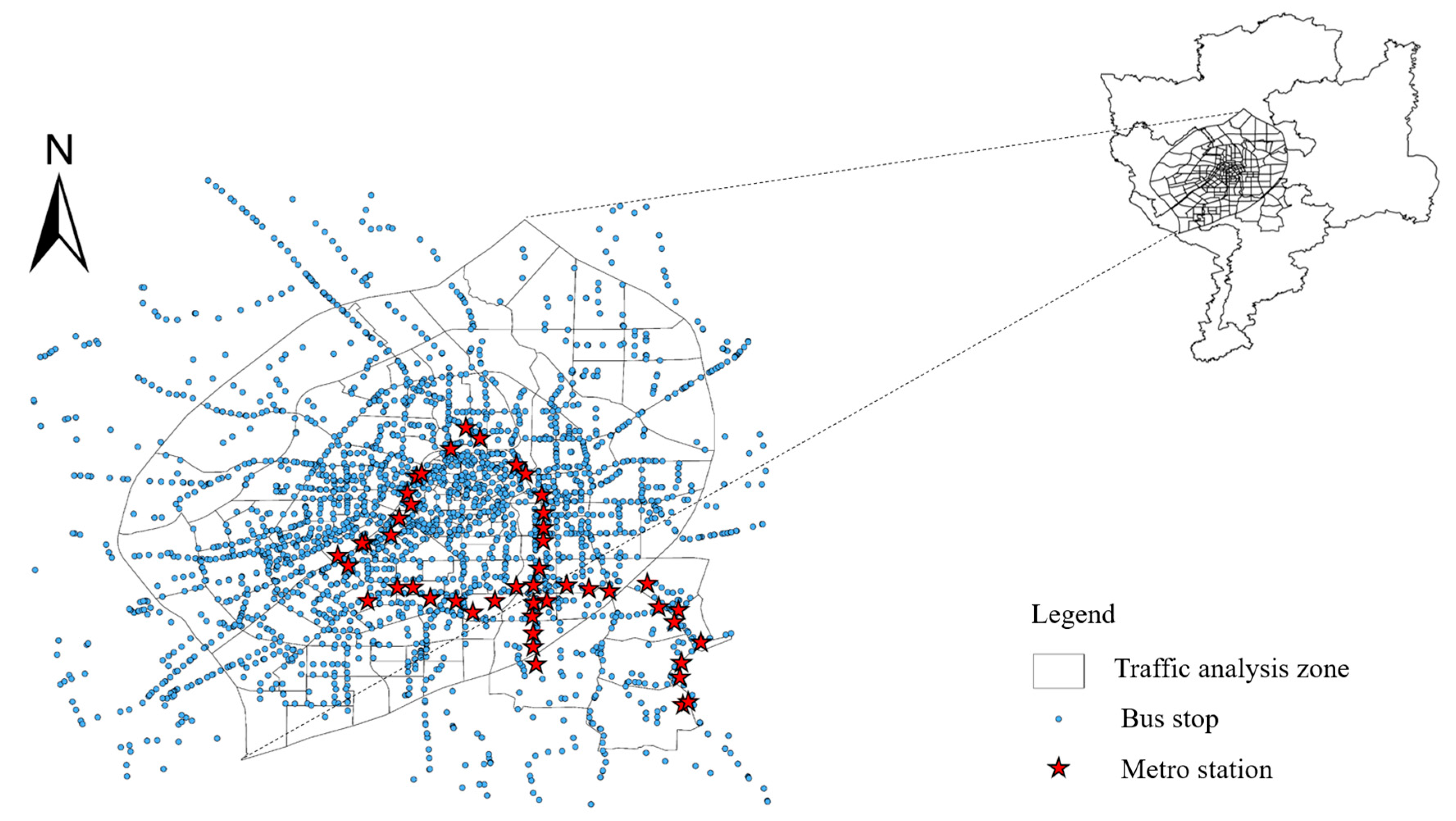
We use Changchun as the study region as shown in Figure 1. It is a mid-size city in Northeast China. Changchun covers approximately 20,565 km2 and is home to a population of more than 7 million as of 2013 [3]. As the capital of Jilin province, Changchun has experienced rapid economic growth and urban expansion. With the rapid development of urbanization, the urban car ownership has grown to more than 1 million until 2013 [3]. The rapid growth causes a series of traffic problems. Therefore, the city is chosen to serve as a reference for similar cities in China.
The primary data is drawn from the 2015 Changchun household travel survey and integrated into the travel model report, which was released by the Beijing Transport Institute. The survey interviews of travel information were conducted by the Beijing Transport Institute from 1 May 2012 to 13 May 2012 to collect all household members’ complete travel information on an assigned workday in Changchun, which is representative of the city. The total sample of the travel survey is 0.68%. The total travel information includes the complete travel information of 51,909 members from 20,000 households for 24 h in Changchun. In total, 3651 households own one or more than one cars, which takes up 18.2% of the total sample. Moreover, the information collected includes socio-demographic characteristics and travel-related information. After error-checking and clearing the data, we selected the commuting trip data from the respondents’ valid questionnaires. Only the commuting trips where the home origin is included. The final sample includes 24,321 commuting trips used for this study.
The socio-demographic data collected includes the respondent’s gender, age, household size, education, Hukou, yearly household income, and household car ownership status.
To examine the impact of the built environment on car ownership and use for commuting, the built environment is measured at the TAZ level according to the location of respondent’s residence. Built environment variables used for analysis include residential density, land use mixture, distance to CBD, bus stop density, and intersection density. Specifically, residential density is obtained by analyzing data from the 6th National Population Census using ArcGIS software. Furthermore, distance to CBD is a variable describing the location characteristics of residence or workplace, which is obtained by calculating the Euclidean distance between the residence and CBD by using ArcGIS software. The bus stop density is obtained using kernel density estimation in ArcGIS software to measure the public transportation accessibility data, which is extracted from the Baidu map application through API (Application Programming Interface). The intersection density is calibrated to measure the street network characteristic based on the Changchun Traffic Map. Moreover, commuting distance is calibrated using the start and end of the trip on the Baidu map, in which commuting distance is represented by the shortest path as usual [4].
And the land use mixture is measured with the entropy method, which has been used frequently [46]. We use the points of interest (POI) data extracted from the Baidu Map to measure the land use mixture at the TAZ level rather than land use data due to the lack of data, which has proven to be effective for measuring land use mixture. The POI data extracted includes residences, hotels, restaurants, supermarkets, parks, squares, malls, schools, hospitals, banks and government departments. The land use mixture can be calibrated as follows:
where is the proportion of the ith POI in traffic analysis zone j. And is the number of POI types existing in traffic analysis zone j.
Variable names and descriptions used for analysis are shown in Table 2.
4. Methodology
The analysis was twofold. First, we examined how the built environment influenced car ownership. Then we analyzed the impacts of the built environment on whether the respondent commuted by car or not. In addition, socio-demographic characteristics were included in the analysis. We employed the Bayesian hierarchical approach with spatial random effects to model the spatial context in which the spatial heterogeneity and autocorrelation can be captured simultaneously. In the models, the multilevel structure was proven to be effective in accounting for the spatial heterogeneity of hierarchical data [40] and the CAR model was employed to specify the spatial autocorrelation at the TAZ level specifically. The proposed models assume that observations at nearby locations tend to have similar characteristics and TAZs vary as a function of built environment variables measured at the TAZ level. The detail models are described as follows.
4.1. Car Ownership Model
The component model is constructed in order to analyze how the built environment affects the car ownership in a household after controlling for socio-demographic variables. The endogenous variable is defined as a binary variable depending on whether the household owns cars or not. Then the Bayesian multilevel binary logistic model can be written as follows:
where is the probability of the household i located in TAZ h owns one or more cars. and are the socio-demographic variables and built environment variables respectively. and are the coefficients to be calibrated. is the varying intercept. Then the CAR model is used to recognize the spatial autocorrelation. And is the spatial random effect to specify the spatial autocorrelation measured at TAZ level, which is shown below.
where is the number of neighbors of traffic analysis zone . is a spatial adjacent matrix indicating the location relation of TAZ and TAZ is below.
Therefore, the final Bayesian multilevel binary logistic model considering spatial autocorrelation of the car ownership component model is as follows.
4.2. Car Use Models
In this section, the model aims to examine the impacts of built environment on car use for commuting. Besides the built environment and socio-demographic characteristics, car ownership status is treated as a binary variable in the model. The final model is shown below.
where is the probability of the commuter i living in TAZ h choosing the car as a commuting mode. is the car ownership status of the household.
The Bayesian approach can be solved based on Bayes’ Theorem as shown below.
where is the posterior distribution. is the conditional probability and the is the prior distribution. In the Bayesian approach, the prior distributions for parameters are needed. However, the prior distributions for the parameters do not exist in this study. Therefore, we used non-informative priors and estimated posterior distributions based on MCMC (Markov Chain Monte Carlo) method. Based on the Bayesian approach, the uncertainty can be obtained by estimating the parameter. It can provide a specific CI (Confidence Interval) for the parameter to be estimated. If zero is not included in the 95% CI, it may be that the endogenous variable impacts the endogenous variable at the 0.05 level of significance.
DIC (Deviance Information Criterion) is used to represent the goodness of fit and complexity. It can be calibrated as seen below.
where is the Bayesian variance of . is the posterior mean of used to represent the goodness of fit. is the number of parameters representing the complexity.
5. Results
The parameters were estimated based on the MCMC method shown in Table 3 and Table 4. We used Gibbs samplers to estimate the fixed and random component in the chain. Additionally, non-informative priors were used for the estimation. MCMC chains were run for 20,000 iterations in this study. In the results, the factors have significant impacts on the endogenous variable at the 0.05 level of significance if zero is included in the 95% CI. Therefore, it can be seen that the CAR effect in the models are both significant at the 0.05 level, which indicates that there exists spatial correlation in the car ownership and use for commuting. Moreover, The DIC values of two models are 2291.45 and 1828.96, respectively.
5.1. Car Ownership Model
According to the results presented in Table 3, the spatial autocorrelation parameter is found to be significant. The result indicates that household car ownership at nearby locations is similar rather than independent.
All socio-demographic coefficients included in this component model show statistical significance. For instance, the results indicate that higher household income and bigger household size is significantly related to a higher probability of owning cars, which is consistent with most prior studies [32]. It has been well-studied that household income closely linked with car maintenance and daily use [21]. Moreover, bigger household size means that there are more children and elder people in the family so it might generate more driving demands for education and healthcare purposes. In addition, these travel purposes usually pose greater convenience and safety concerns. Furthermore, households with local Hukou are more likely to own cars, which may explain that people owning local Hukou enjoy better social welfare than those without local Hukou.
After controlling for the socio-demographic variables, some built environment variables also are found to play an important role in explaining the household car ownership. The residential density has significant negative effects on car ownership. It may be due to the fact that the residence with a higher residential density has a higher probability of being located in a neighborhood concentrated with more activities, facilities, and services. Therefore, more travel purposes can be met in the neighborhood, which leads to less car travel demand. Land use mixture is found to be negatively associated with car ownership. Thanks to compact land use, it is more likely that the trip origin and destination are close, which raises the probability of non-motorized travel rather than car. On the other hand, distance to CBD is a factor that shows no significant effects on car ownership, which is a different conclusion from previous studies [67]. This means that the location of residence is not correlated with household car ownership. This may be because, while car ownership is growing rapidly in Changchun, the car ownership of households is mainly restricted by economic status and other factors and not related with residence location when compared with car-dependent countries. The factor of bus stop density has negative effects on car ownership and the reason for this might be that the household can have more travel choices when they live close to transit. Moreover, the household is less likely to own cars when the neighborhood has a higher intersection density.
5.2. Car Use Model
The results are presented in Table 4 for the car use model and the spatial autocorrelation parameter is found to be significant. The result indicates that car use for the journey to work of commuters has a similar trend at nearby locations.
In the car use model, we implement the joint analysis of the impacts of built environment characteristics and socio-demographic characteristics on car use. The results of commuters’ mode choice model for the journey to work are shown in Table 4. We can see that the socio-demographic variables include household income, car ownership, gender, and Hukou, which have significant influence on car use for commuters. For example, people from high-income households tend to drive to work more. Men are, in particular, more likely to drive to work, which is consistent with previous studies [62]. However, the age and education are found to be insignificant when compared to car use for the journey to work. Moreover, there is no significant influence in household size on the commuting mode. Though it is widely known that bigger household size can generate more car travel, this finding may be explained by people with a bigger household using cars more often for non-commuting purposes such as education, hospital, and shopping instead of commuting.
The results on built environment characteristics in Table 4 indicate that most built environment variables show a significant relationship with the travel mode for work when other characteristics are controlled. People living in a neighborhood with high residential density are more likely get to work by other modes of travel besides driving. Land use mixture was found to be significantly associated with using cars to commute to work at the 95% level, which is consistent with studies conducted by Ding et al. [23]. This might be explained by the neighborhood land use mixture generating more non-motorized travel for non-commuting purposes because the compact land use provides a higher probability for shorter travel distance to shops and hospitals, but not significantly for commuting purposes [67]. Distance to CBD is another factor influencing car use significantly. People who live far from to CBD, commute by car more often. It may be due to the fact that more employment opportunities surround CBD, which raises the commuting distance for people living farther. Bus stop density is a built environment factor that can significantly help reduce car use for commuting. It is an important index measuring the public transit service level in Chinese cities. As the bus stop density increases, the odds of people commuting by car become lower. This means that if there are more public transit facilities supplied, people have a higher probability of choosing public transit as a commuting mode. It indicates that public transit facilities actually prevent people from driving to work. On the other hand, it is possible that transportation planners tend to provide more perfect transit service where residents prefer to travel by transit. It is found that, as the intersection density increases, the odds of commuting by car are lower. This may be due to people having better access for walking, cycling, and public transit, which reduces car use for commuting to work.
6. Conclusions
In this study, Bayesian multilevel binary logistic models incorporating impact analysis and spatial random effects were employed to investigate the influences of the built environment on car ownership and use in Changchun, China. Moreover, the spatial autocorrelation of car ownership and use for commuting across TAZs was recognized, and the impacts of the built environment on car ownership and use for commuting influences were confirmed.
The data used for analysis in this study came from multiple sources. The travel data was collected from the household travel survey in Changchun. The built environment data was collected at the TAZ level in Changchun including residential density, land use mixture, distance to CBD, bus stop density and intersection density. Based on the data, Bayesian multilevel binary logistic models are employed for investigating the determinants of car ownership and use for commuting considering socio-demographic characteristics and built environment characteristics. Meanwhile, the spatial autocorrelation of car ownership and use across TAZs was recognized in the models. The findings are summarized below.
The empirical study provided important benefits in recognizing the spatial autocorrelation of car ownership and use across TAZs. The estimated results indicate that the unobserved spatial effects of car ownership and use for commuting both exist. There are similar trends among household car ownership and commuters’ car use for the journey to work at nearby locations. Therefore, urban planners and transportation policy makers need to better understand substantive and technical implications of dependence and create sustainable land use development policy.
For the effects of socio-demographic characteristics, the decision of car ownership and use was influenced by most factors. More attention should be paid to people with local Hukou since the results suggest that local Hukou increases the probability of driving for journeys to work while, reducing the likelihood of public transit and other modes. Hukou is a special system to control the population movement from rural area to cities in China, which can prevent people from a few social benefits. The mobile population returned 200 million people until 2016 in China [68]. The Chinese government is actively promoting the reform household registration system to encourage reasonable population movement. Moreover, apart from large cities in China, people without local Hukou are often rural migrant workers in small and mid-sized cities who have lower desire to purchase cars. Therefore, with large crowds of people moving into cities, city administration officials should make some effort to develop quota control policy especially for commuters with local Hukou to slow the growth of car ownership and use.
Due to the increasing interests in considering land use planning as a tool for reducing travel energy use and emissions, this study provided new evidence for how built environment characteristics influence car ownership and use for commuting. The estimated results indicated that the built environment actually played an important role in influencing car ownership and use after controlling for socio-demographic characteristics. Due to the different attributes in the built environment, economy, and social structures, the impact of the built environment on car ownership and use vary among different national contexts. It is clear that distance to CBD shows no significant impact on car ownership in Changchun. Therefore, car ownership and use control policy needs to be developed based on local conditions. However, there are some similar results with prior studies conducted in western countries [16,22,23,24,40]. It was found that residential density, land use mixture, bus stop density, and intersection density had significant effects on household car ownership. Moreover, higher residential density, bus stop density, and intersection density were important factors that could help reduce car use for commuting to work. On the other hand, longer distance to CBD could generate more time commuting by car. Therefore, it might be feasible to reduce car ownership and use for commuting by using land use planning policy including creating higher residential density, improving public transit investment, designing better street connectivity, and proposing job-housing balancing policy.
Given the increased debates on the energy and environmental problems, urban planners and transportation policy makers can develop strategies to reduce car ownership and use based on the influence mechanisms of the built environment in developing counties. This study can provide additional insight into the relationship between land use development and sustainable mobility behavior and further provide theoretical support for the transit-oriented development (TOD) in developing countries.
Future work will be focused on the following aspects. First, the built environment of destination should be incorporated for analyzing car use for commuting for follow up work. In addition, future studies may integrate more public transit characteristics into the model, because public transit has attracted a huge investment in China, where the influence on car ownership and use should not be neglected.
Acknowledgments
This work was supported by the Hebei Natural Science Foundation under Grant E2016513016 and the Fundamental Research Funds for the Central Universities under 2017YJS103.
Author Contributions
In this paper, Xiaoquan Wang proposed the idea, designed the algorithm and wrote the paper; Chunfu Shao provided guidance, comments and key suggestions; Chaoying Yin collected and analyzed the built environment data; Chengxiang Zhuge and Wenjun Li proposed improved advice for the paper.
Conflicts of Interest
The authors declare no conflict of interest.
References
- Zhang, Y.; Wu, W.; Li, Y.; Liu, Q.; Li, C. Does the built environment make a difference? An investigation of household vehicle use in Zhongshan metropolitan area, China. Sustainability 2014, 6, 4910–4930. [Google Scholar] [CrossRef]
- Wu, W.; Hong, J. Does public transit improvement affect commuting behavior in Beijing, China? A spatial multilevel approach. Transp. Res. Part D 2016, 52, 471–479. [Google Scholar] [CrossRef]
- National Bureau of Statistics. China Statistic Yearbook 2014; China Statistics Press: Beijing, China, 2014.
- Zhang, M.; Zhao, P. The impact of land-use mix on residents’ travel energy consumption: New evidence from Beijing. Transp. Res. Part D 2017, 57, 224–236. [Google Scholar] [CrossRef]
- Badland, H.M.; Garrett, N.; Schofield, G.M. How does car parking availability and public transport accessibility influence work-related travel behaviors? Sustainability 2010, 2, 576–590. [Google Scholar] [CrossRef]
- Wang, B.; Shao, C.; Ji, X. Influencing mechanism analysis of holiday activity–travel patterns on transportation energy consumption and emissions in china. Energies 2017, 10, 897–916. [Google Scholar] [CrossRef]
- Yang, Z.; Jia, P.; Liu, W.; Yin, H. Car ownership and urban development in Chinese cities: A panel data analysis. J. Transp. Geogr. 2017, 58, 127–134. [Google Scholar] [CrossRef]
- Cao, X.; Huang, X. City-level determinants of private car ownership in China. Asian Geogr. 2013, 30, 37–53. [Google Scholar] [CrossRef]
- Huang, X.; Cao, X.; Yin, J.; Cao, X. Effects of metro transit on the ownership of mobility instruments in Xi’an, China. Transp. Res. Part D 2017, 52, 495–505. [Google Scholar] [CrossRef]
- Jiang, Y.; Gu, P.; Chen, Y.; He, D.; Mao, Q. Influence of land use and street characteristics on car ownership and use: Evidence from Jinan, China. Transp. Res. Part D 2017, 52, 518–534. [Google Scholar] [CrossRef]
- Cervero, R. The built environment and travel: Evidence from the United States. Eur. J. Transp. Infrastruct. Res. 2003, 3, 119–137. [Google Scholar]
- Cervero, R. Built environments and mode choice: Toward a normative framework. Transp. Res. Part D 2002, 7, 265–284. [Google Scholar] [CrossRef]
- Ewing, R.; Cervero, R. Travel and the built environment: A meta-analysis. J. Am. Plan. Assoc. 2010, 76, 265–294. [Google Scholar] [CrossRef]
- Cao, X. Exploring causal effects of neighborhood type on walking behavior using stratification on the propensity score. Environ. Plan. A 2010, 42, 487–504. [Google Scholar] [CrossRef]
- Cao, X.; Mokhtarian, P.L.; Handy, S.L. The relationship between the built environment and non-work travel: A case study of northern California. Transp. Res. Part A 2009, 43, 548–559. [Google Scholar] [CrossRef]
- Ding, C.; Lin, Y.; Liu, C. Exploring the influence of built environment on tour-based commuter mode choice: A cross-classified multilevel modeling approach. Transp. Res. Part D 2014, 32, 230–238. [Google Scholar] [CrossRef]
- Ding, C.; Mishra, S.; Lu, G.; Yang, J.; Liu, C. Influences of built environment characteristics and individual factors on commuting distance: A multilevel mixture hazard modeling approach. Transp. Res. Part D 2017, 51, 314–325. [Google Scholar] [CrossRef]
- Aditjandra, P.T. The impact of urban development patterns on travel behavior: Lessons learned from a British metropolitan region using macro-analysis and micro-analysis in addressing the sustainability agenda. Res. Transp. Bus. Manag. 2013, 7, 69–80. [Google Scholar] [CrossRef]
- Aditjandra, P.T.; Mulley, C.; Nelson, J.D. The influence of neighbourhood design on travel behaviour: Empirical evidence from North East England. Transp. Policy 2013, 26, 54–65. [Google Scholar] [CrossRef]
- Aditjandra, P.T.; Mulley, C.; Nelson, J.D. Extent to Which Sustainable Travel to Work Can Be Explained by Neighborhood Design Characteristics. Transp. Res. Rec. J. Transp. Res. Board 2009, 2134, 114–122. [Google Scholar] [CrossRef]
- Wang, D.; Zhou, M. The built environment and travel behavior in urban China: A literature review. Transp. Res. Part D 2016, 52, 574–585. [Google Scholar] [CrossRef]
- Ding, C.; Liu, C.; Zhang, Y.; Yang, J.; Wang, Y. Investigating the impacts of built environment on vehicle miles traveled and energy consumption: Differences between commuting and non-commuting trips. Cities 2017, 68, 25–36. [Google Scholar] [CrossRef]
- Ding, C.; Wang, Y.; Yang, J.; Liu, C.; Lin, Y. Spatial heterogeneous impact of built environment on household auto ownership levels: Evidence from analysis at traffic analysis zone scales. Transp. Lett. Int. J. Transp. Res. 2016, 8, 26–34. [Google Scholar] [CrossRef]
- Ding, C.; Wang, Y.; Xie, B.; Liu, C. Understanding the role of built environment in reducing vehicle miles traveled accounting for spatial heterogeneity. Sustainability 2014, 6, 589–601. [Google Scholar] [CrossRef]
- Zhao, P. Private motorized urban mobility in china’s large cities: The social causes of change and an agenda for future research. J. Transp. Geogr. 2014, 40, 53–63. [Google Scholar] [CrossRef]
- Hong, J.; Chen, C. The role of the built environment on perceived safety from crime and walking: Examining direct and indirect impacts. Transportation 2014, 41, 1171–1185. [Google Scholar] [CrossRef]
- Hong, J.; Goodchild, A. Land use policies and transport emissions: Modeling the impact of trip speed, vehicle characteristics and residential location. Transp. Res. Part D 2014, 26, 47–51. [Google Scholar] [CrossRef]
- Hong, J.; Shen, Q. Residential density and transportation emissions: Examining the connection by addressing spatial autocorrelation and self-selection. Transport. Res. Part D 2013, 22, 75–79. [Google Scholar] [CrossRef]
- Cervero, R.; Kockelman, K. Travel demand and the 3ds: Density, diversity, and design. Transp. Res. Part D 1997, 2, 199–219. [Google Scholar] [CrossRef]
- Cervero, R.; Lsarmiento, O.; Jacoby, E.; Gomez, L.F.; Nei-Man, A.; Xue, G. Influences of built environments on walking and cycling: Lessons from Bogotá. Int. J. Sustain. Transp. 2009, 3, 203–226. [Google Scholar] [CrossRef]
- Shay, E.; Khattak, A. Automobiles, trips, and neighborhood type: Comparing environmental measures. Transp. Res. Rec. J. Transp. Res. Board 2007, 2010, 73–82. [Google Scholar] [CrossRef]
- Li, S.; Zhao, P. Exploring car ownership and car use in neighborhoods near metro stations in Beijing: Does the neighborhood built environment matter? Transport. Res. Part D 2017, 56, 1–17. [Google Scholar] [CrossRef]
- Frank, L.D. Impacts of mixed used and density on utilization of three modes of travel: Single-occupant vehicle, transit, walking. Transp. Res. Rec. J. Transp. Res. Board 1994, 1466, 44–52. [Google Scholar]
- Boarnet, M.G.; Sarmiento, S. Can land-use policy really affect travel behavior? A study of the link between non-work travel and land-use characteristics. Urban Stud. 1996, 35, 1155–1169. [Google Scholar] [CrossRef]
- Crane, R. Cars and drivers in the new suburbs: Linking access to travel in neo-traditional planning. Univ. Calif. Transp. Center Work. Pap. 1994, 62, 51–65. [Google Scholar] [CrossRef]
- Potoglou, D.; Kanaroglou, P.S. Modelling car ownership in urban areas: A case study of Hamilton, Canada. J. Transp. Geogr. 2008, 16, 42–54. [Google Scholar] [CrossRef]
- Acker, V.V.; Witlox, F. Car ownership as a mediating variable in car travel behavior research using a structural equation modelling approach to identify its dual relationship. J. Transp. Geogr. 2010, 18, 65–74. [Google Scholar] [CrossRef] [Green Version]
- Zegras, C. The built environment and motor vehicle ownership and use: Evidence from Santiago de Chile. Urban Stud. 2010, 47, 1793–1817. [Google Scholar] [CrossRef]
- Hong, J.; Shen, Q.; Zhang, L. How do built-environment factors affect travel behavior? A spatial analysis at different geographic scales. Transportation 2014, 41, 419–440. [Google Scholar] [CrossRef]
- Ding, C.; Wang, D.; Liu, C.; Zhang, Y.; Yang, J. Exploring the influence of built environment on travel mode choice considering the mediating effects of car ownership and travel distance. Transp. Res. Part A 2017, 100, 65–80. [Google Scholar] [CrossRef]
- Zhang, L.; Hong, J.H.; Nasri, A.; Shen, Q. How built environment affects travel behavior: A comparative analysis of the connections between land use and vehicle miles traveled in US cities. J. Transp. Land Use 2012, 5, 40–52. [Google Scholar] [CrossRef]
- Wheeler, S.M.; Tomuta, M.; Haden, V.R.; Jackson, L.E. The impacts of alternative patterns of urbanization on greenhouse gas emissions in an agricultural county. J. Urban Int. Res. Placemak. Urban Sustain. 2013, 6, 213–235. [Google Scholar] [CrossRef]
- Dargay, J.; Gately, D. Income’s effect on car and vehicle ownership, worldwide: 1960–2015. Transp. Res. Part A 1999, 33, 101–138. [Google Scholar] [CrossRef]
- Jong, G.D.; Fox, J.; Daly, A.; Pieters, M.; Smit, R. Comparison of car ownership models. Transp. Rev. 2004, 24, 379–408. [Google Scholar] [CrossRef]
- Paulley, N.; Balcombe, R.; Mackett, R.; Titheridge, H.; Preston, J.; Wardman, M.; Shires, J.; White, P. The demand for public transport: The effects of fares, quality of service, income and car ownership. Transp. Policy 2006, 13, 295–306. [Google Scholar] [CrossRef]
- Cao, X.; Yang, W. Examining the effects of the built environment and residential self-selection on commuting trips and the related CO2 emissions: An empirical study in Guangzhou, China. Transp. Res. Part D 2017, 52, 480–494. [Google Scholar] [CrossRef]
- Schmale, J.; Schneidemesser, E.V.; Dörrie, A. An integrated assessment method for sustainable transport system planning in a middle sized German city. Sustainability 2015, 7, 1329–1354. [Google Scholar] [CrossRef]
- Giuliano, G.; Dargay, J. Car ownership, travel and land use: A comparison of the USA and Great Britain. Transp. Res. Part A 2006, 40, 106–124. [Google Scholar] [CrossRef]
- Raphael, S.; Rice, L. Car ownership, employment, and earnings. J. Urban Econ. 2000, 52, 109–130. [Google Scholar] [CrossRef]
- Wang, T.; Chen, C. Impact of fuel price on vehicle miles traveled (VMT): Do the poor respond in the same way as the rich? Transportation 2014, 41, 91–105. [Google Scholar] [CrossRef]
- Heres-Del-Valle, D.; Niemeier, D. Co emissions: Are land-use changes enough for California to reduce VMT? Specification of a two-part model with instrumental variables. Transp. Res. Part B Meth. 2011, 45, 150–161. [Google Scholar] [CrossRef]
- Ballard, K.J.; Robin, D.A.; Woodworth, G.; Zimba, L.D. Age-related changes in motor control during articulator visuomotor tracking. J. Speech Lang. Hear. Res. 2001, 44, 763–777. [Google Scholar] [CrossRef]
- Aditjandra, P.T.; Cao, X.; Mulley, C. Understanding neighbourhood design impact on travel behaviour: An application of structural equations model to a British metropolitan data. Transp. Res. Part A 2012, 46, 22–32. [Google Scholar] [CrossRef]
- Xu, T.; Zhang, M.; Aditjandra, P.T. The impact of urban rail transit on commercial property value: New evidence from Wuhan, China. Transp. Res. Part A 2016, 91, 223–235. [Google Scholar] [CrossRef]
- Wang, X.; Yuan, J. Safety Impacts Study of Roadway Network Features on Suburban Highways. China J. Highw. Transp. 2017, 30, 106–114. [Google Scholar]
- Chen, X.; Zhang, H. Evaluation of effects of car ownership policies in Chinese megacities. Transp. Res. Rec. J. Transp. Res. Board 2012, 2317, 32–39. [Google Scholar] [CrossRef]
- Li, J.; Walker, J.L.; Inivasan, S.; Anderson, W.P. Modeling private car ownership in China. Transp. Res. Rec. J. Transp. Res. Board 2010, 2193, 76–84. [Google Scholar] [CrossRef]
- Wu, N.; Zhao, S.; Zhang, Q. A study on the determinants of private car ownership in China: Findings from the panel data. Transp. Res. Part A 2016, 85, 186–195. [Google Scholar] [CrossRef]
- Pan, H.; Shen, Q.; Zhao, T. Travel and car ownership of residents near new suburban metro stations in Shanghai, China. Transp. Res. Rec. J. Transp. Res. Board 2013, 2394, 63–69. [Google Scholar] [CrossRef]
- Zhang, R.; Yao, E.; Liu, Z. School travel mode choice in Beijing, China. J. Transp. Geogr. 2017, 62, 98–110. [Google Scholar] [CrossRef]
- Jiang, Y.; Zegras, P.C.; He, D.; Mao, Q. Does energy follow form? The case of household travel in Jinan, China. Mitig. Adapt. Strateg. Glob. Chang. 2015, 20, 701–718. [Google Scholar] [CrossRef]
- Sun, B.; Ermagun, A.; Dan, B. Built environmental impacts on commuting mode choice and distance: Evidence from Shanghai. Transp. Res. Part D 2017, 52, 441–453. [Google Scholar] [CrossRef]
- Liu, Q.; Wang, J.; Chen, P.; Xiao, Z. How does parking interplay with the built environment and affect automobile commuting in high-density cities? A case study in China. Urban Stud. 2016. [Google Scholar] [CrossRef]
- Zhao, P. The impact of the built environment on individual workers’ commuting behavior in Beijing. Int. J. Sustain. Transp. 2013, 7, 389–415. [Google Scholar] [CrossRef]
- Cervero, R.; Jin, M. Effects of built environments on vehicle miles traveled: Evidence from 370 US urbanized areas. Environ. Plan. A 2010, 42, 400–418. [Google Scholar] [CrossRef]
- Christiansen, P.; Engebretsen, Ø.; Fearnley, N.; Hanssen, J.U. Parking facilities and the built environment: Impacts on travel behavior. Transp. Res. Part A 2017, 95, 198–206. [Google Scholar] [CrossRef]
- Ding, C.; Wang, Y.; Tang, T.; Mishra, S.; Liu, C. Joint analysis of the spatial impacts of built environment on car ownership and travel mode choice. Transp. Res. Part D 2016. [Google Scholar] [CrossRef]
- National Bureau of Statistics. China Statistic Yearbook 2017; China Statistics Press: Beijing, China, 2017.
Figure 1.
Study region and traffic analysis zones.

Table 1.
Summary of existing studies on impacts of built environment and car dependency.
| Location | Method | Content | Reference |
|---|---|---|---|
| Baltimore, MD, USA | Structural equation | Car use | [22] |
| Washington, DC, USA | Multilevel ordered probit | Car ownership | [23] |
| Hamilton, ON, Canada | Ordered logit | Car ownership | [36] |
| Ghent, Belgium | Structural equation | Car ownership and use | [37] |
| Santiago de, Chile | Multinomial logit and ordinary least squares regression | Car ownership and use | [38] |
| America | Structural equation | Car use | [50] |
| Britain | Structural equation | Car use | [53] |
| America | Structural equation | Car use | [65] |
| Norway | Logistic regression | Car ownership and use | [66] |
| Zhongshan, China | Negative binomial regression | Car use | [1] |
| Beijing, China | Logistic regression and negative binomial regression | Car ownership and use | [32] |
| Shanghai, China | Logistic regression | Car ownership and use | [59] |
| Shenzhen, China | Structural equation | Car ownership and use | [63] |
Table 2.
Variables and descriptions used for analysis.
| Variables | Description | Mean | Standard Deviation |
|---|---|---|---|
| socio-demographics characteristics | |||
| Gender | Male (1 = yes; 0 = otherwise) | 0.62 | 0.48 |
| Age | Age in years | 38.16 | 10.74 |
| Education | Completed college degree (1 = yes; 0 = otherwise) | 0.37 | 0.48 |
| Household size | Numbers of household members | 2.72 | 1.04 |
| Hukou | Local Hukou (1 = yes; 0 = otherwise) | 0.86 | 0.34 |
| Income 1 | Yearly household income in RMB: 20,000 and less | 0.20 | 0.16 |
| Income 2 | Yearly household income in RMB: 20,000–100,000 | 0.77 | 0.18 |
| Income 3 | Yearly household income in RMB: 100,000 and more | 0.03 | 0.03 |
| Car ownership | One or more cars (1 = yes; 0 = otherwise) | 0.22 | 0.17 |
| Built environment characteristics | |||
| Residential density | Residential density per square kilometer at TAZ level | 0.34 | 0.22 |
| Land use mixture | Measurement of degree of different types of land use composition | 0.59 | 0.17 |
| Distance to CBD | Distance to CBD in kilometers | 4.8 | 2.91 |
| Bus stop density | Bus stop density per square kilometer at TAZ level | 10.50 | 5.91 |
| Intersection density | Intersection density per square kilometer at TAZ level | 33.38 | 17.83 |
| Travel-related characteristics | |||
| Commuting mode | Private car (1 = yes; 0 = otherwise) | 0.11 | 0.09 |
Table 3.
Estimated results of car ownership model.
| Variables | Mean | 95% CI | |
|---|---|---|---|
| 2.5% | 97.5% | ||
| socio-demographics at individual level | |||
| Household Size | 0.05 | 0.01 | 0.12 |
| Hukou | 1.82 | 1.58 | 2.08 |
| Income 2 | 0.21 | 0.09 | 0.33 |
| Income 3 | 0.75 | 0.60 | 0.91 |
| Built environment at TAZ level | |||
| Residential density | −0.10 | −0.17 | −0.03 |
| Land use mixture | −0.07 | −0.10 | −0.05 |
| Distance to CBD | 0.14 | −0.07 | 0.35 |
| Bus stop density | −0.03 | −0.05 | −0.01 |
| Intersection density | −0.21 | −0.32 | −0.11 |
| 0.18 | 0.03 | 0.52 | |
| 0.46 | 0.16 | 0.98 | |
| DIC | 2291.45 | ||
Table 4.
Estimated results of car use model for journey to work.
| Variables | Mean | 95% CI | |
|---|---|---|---|
| 2.5% | 97.5% | ||
| Socio-demographics at individual level | |||
| Household size | 0.21 | −0.10 | 0.53 |
| Income 2 | 0.19 | 0.09 | 0.30 |
| Income 3 | 1.23 | 1.01 | 1.46 |
| Car ownership | 0.94 | 0.79 | 1.09 |
| Gender | 0.34 | 0.13 | 0.55 |
| Age | −0.05 | −0.10 | 0.02 |
| Education | 0.09 | −0.07 | 0.25 |
| Hukou | 1.41 | 0.47 | 2.37 |
| Built environment at TAZ level | |||
| Residential density | −0.74 | −0.96 | −0.52 |
| Land use mixture | 0.17 | −0.10 | 0.44 |
| Distance to CBD | 0.09 | 0.05 | 0.13 |
| Bus stop density | −0.15 | −0.24 | −0.06 |
| Intersection density | −0.11 | −0.05 | −0.17 |
| 1.23 | 0.98 | 1.49 | |
| 0.57 | 0.27 | 0.85 | |
| DIC | 1989.93 | ||
© 2018 by the authors. Licensee MDPI, Basel, Switzerland. This article is an open access article distributed under the terms and conditions of the Creative Commons Attribution (CC BY) license (http://creativecommons.org/licenses/by/4.0/).
Share and Cite
MDPI and ACS Style
Wang, X.; Shao, C.; Yin, C.; Zhuge, C.; Li, W. Application of Bayesian Multilevel Models Using Small and Medium Size City in China: The Case of Changchun. Sustainability 2018, 10, 484. https://doi.org/10.3390/su10020484
AMA Style
Wang X, Shao C, Yin C, Zhuge C, Li W. Application of Bayesian Multilevel Models Using Small and Medium Size City in China: The Case of Changchun. Sustainability. 2018; 10(2):484. https://doi.org/10.3390/su10020484
Chicago/Turabian StyleWang, Xiaoquan, Chunfu Shao, Chaoying Yin, Chengxiang Zhuge, and Wenjun Li. 2018. "Application of Bayesian Multilevel Models Using Small and Medium Size City in China: The Case of Changchun" Sustainability 10, no. 2: 484. https://doi.org/10.3390/su10020484
Note that from the first issue of 2016, this journal uses article numbers instead of page numbers. See further details here.