Influence of Sampling Point Discretization on the Regional Variability of Soil Organic Carbon in the Red Soil Region, China

Abstract

Research on the regional variability of soil organic carbon (SOC) has focused mostly on the influence of the number of soil sampling points and interpolation methods. Little attention has typically been paid to the influence of sampling point discretization. Based on dense soil sampling points in the red soil area of Southern China, we obtained four sample discretization levels by a resampling operation. Then, regional SOC distributions were obtained at four levels by two interpolation methods: ordinary Kriging (OK) and Kriging combined with land use information (LuK). To evaluate the influence of sample discretization on revealing SOC variability, we compared the interpolation accuracies at four discretization levels with uniformly distributed validation points. The results demonstrated that the spatial distribution patterns of SOC were roughly similar, but the contour details in some local areas were different at the various discretization levels. Moreover, the predicted mean absolute errors (MAE) and root mean square errors (RMSE) of the two Kriging methods all rose with an increase in discretization. From the lowest to the largest discretization level, the MAEs of OK and LuK rose from 4.47 and 3.02 g kg⁻¹ to 5.46 and 3.54 g kg⁻¹, and the RMSEs rose from 5.13 and 3.95 g kg⁻¹ to 5.76 and 4.76 g kg⁻¹, respectively. Though the trend of prediction errors varied with discretization levels, the interpolation accuracies of the two Kriging methods were both influenced by the sample discretization level. Furthermore, the spatial interpolation uncertainty of OK was more sensitive to the discretization level than that of the LuK method. Therefore, when the spatial distribution of SOC is predicted using Kriging methods based on the same sample quantity, the more uniformly distributed sampling points are, the more accurate the spatial prediction accuracy of SOC will be, and vice versa. The results of this study can act as a useful reference for evaluating the uncertainty of SOC spatial interpolation and making a soil sampling scheme in the red soil region of China.

1. Introduction

Soil organic carbon (SOC), as an important soil property, not only directly affects soil fertility and crop growth, but also plays an important role in global carbon cycling [1,2,3]. Generally, regional SOC has a strong spatial variability due to the complex soil forming factors and increasing influence of human activities [4,5,6]. Revealing the characteristics of regional SOC spatial variability accurately is significant for developing reasonable policies for agricultural management and environmental protection.

At present, remote sensing still cannot effectively reveal the distribution characteristics of regional SOC due to the detectability of SOC at certain thicknesses with the sensors available nowadays. Soil field sampling, laboratory testing, and point-to-surface expansion are still the main processes used to determine the spatial distribution characteristics of SOC [7]. In these processes, soil field sampling is the basic link for the follow-up actions. In recent decades, researchers have developed several soil sampling designs for regional soil investigation, including the simple random sampling design, the stratified sampling design, the systematic sampling design [7,8,9,10,11], etc. Because the design principles are different for each sampling design, the spatial distribution features of sampling points are distinctly different between designs. Based on statistical principles, the simple random sampling design randomly takes soil samples from the study area and can ensure that selection occurs without bias. In addition, some researchers have stated that this design can usually estimate the SOC distribution well [8,12]. However, it should be noted that those sampling points obtained with random sampling are often unevenly distributed or overdispersed. Using practical regional soil surveys, some researchers have found obvious differences in SOC content and variability among different soil types, land use patterns, or vegetation types [13,14,15]. As a result, type-based stratified sampling design has been used in regional SOC surveys, such as the soil type-based stratified sampling design, the land use based stratified sampling design, and so on. In these type-based stratified designs, the study area is divided into several different subregions with relatively uniform properties, and then, soil samples are allocated respectively in each subregion according to respective variation characteristics of SOC content. Because the variation features of SOC differ in different subregions, the allocated sampling points by stratified design show usually are densely distributed in some areas and sparsely distributed in other areas. In recent years, systematic sampling with a squared grid has been widely applied in soil surveys owing to the advances in geostatistics and geographic information system (GIS) technology [16,17]. In this design, a well-designed net is superimposed upon the study area on the computer, and sampling points are placed at the central position of each grid. The size of grid can range from square meters to square kilometers according to the research purposes and requirements. Systematic sampling with a squared grid has become increasingly popular in recent years because it can be conveniently operated with GIS software [7]. The soil sampling points allocated by this design are all regularly and uniformly distributed.

Point-to-surface expansion is a critical step in the transition from a limited number of sampling points to a continuous surface distribution map of SOC [18]. To obtain the spatial variation features of regional SOC, the main interpolation methods, including polynomial inter method, polygon-based method, and the Kriging method, have usually been used [19,20,21,22,23]. Among these methods, the polynomial method and the polygon-based method were the main methods used to reveal the SOC distribution and estimate regional carbon storage in the early stages of SOC research. However, with the advances of geostatistics and GIS technology, Kriging has gradually become the dominant method in recent years [24]. To improve the spatial prediction accuracy of SOC, a variety of Kriging methods derived from ordinary Kriging, such as co-Kriging, universal Kriging, regression Kriging, Kriging combined with categorical auxiliary information, and so on [25,26]. During point-to-surface expansion of regional SOC using Kriging methods, the influences of the sample quantity and the method selection on the interpolation accuracy are typical concerns of soil researchers [17], but few researchers have paid attention to the interpolation uncertainty generated by the spatial distribution characteristics of the sampling point.

As the discretization level can characterize the distributed features and interrelation of sampling points in space, it is a commonly used parameter to describing the spatial distribution characteristics of sampling points in geographic and ecological research [27]. In field soil survey sampling, the sampling points obtained by different sampling designs usually do not have the same distribution characteristics. Intuitively, there may be great differences in the spatial discretization levels of sampling points. When using the Kriging method to reveal the spatial variability of SOC, it is unknown whether the magnitude of the sample discretization affects the uncertainty of spatial interpolation, and if so, how great the influence is. At present, there have been few studies on these questions. For this reason, taking the central region of Yujiang County in Jiangxi Province, China as the study area, multiple discretization levels were obtained by a resampling operation based on existing sampling points in this area. Two Kriging methods were used for SOC spatial interpolation, and then, their interpolation uncertainty levels were compared with the various sample discretization levels. The primary objectives of this study were to (1) reveal the influence of the sample discretization level on the interpolation uncertainty in revealing SOC variability, and to find out what kind of discretization is beneficial to spatial interpolation with the Kriging method and (2) to find out the differences in responses to the sample discretization level for the different Kriging methods used for SOC interpolation. The research results will provide a useful reference for revealing spatial variability of regional SOC and making sampling strategies in the hilly region of red soil in China.

2. Materials and Methods

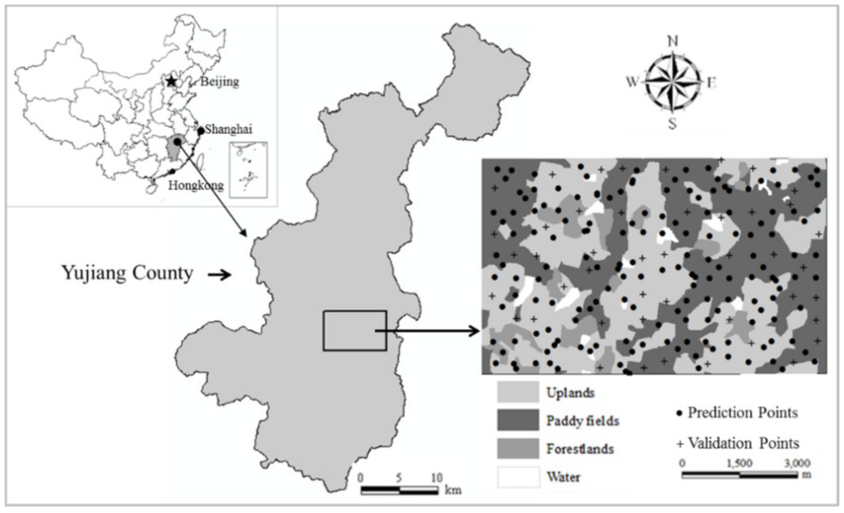
2.1. Study Area

The study area (116°41′–117°09′ E, 28°04′–28°37′ N) is located in the middle area of Yujiang County, and covers a region of 40 km² (8 km × 5 km). Situated in a subtropical, humid monsoon climate zone, the study area has a warm climate, abundant heat and sunshine, plentiful rainfall, and a long frost-free period. The annual average temperature is 17.6 °C, and the annual average precipitation is 1778.8 mm. Its frost-free period is approximately 258 days. The terrain in the study area is dominated by hilly and low mountains. Red soil (acrisols, WRB 2006) [28] is the most important soil type, and the main soil parent materials are red sandstone, quaternary red clay, shale, and river alluvium (Yujiang County, Jiangxi Province Soil Census Office, 1986) [29]. Paddy fields, dry land, and forestland are the major land use patterns. The main crops are rice, grains, sweet potatoes, peanuts, and sesames.

2.2. Soil Sample Collection and Processing

The SOC data used in this research were derived from the soil sampling point database established with supported of the Chinese Academy of Sciences (CAS) project “Soil Quality Grad- determination and Production Potential Assessment”. In this project, the soil samples were collected by stepped grid sampling design in Yujiang County. Some samples were collected in 2 km × 2 km grids across the whole county, some samples were collected in 1 km × 1 km grids within the central region of the county, and some samples were collected in 0.5 km × 0.5 km grids across a 40 km² area within the 1 km × 1 km grid sampling area [30]. In the actual sampling practice, if the sampling point lay in a village, road, or water body, then its position was adjusted and collected nearby. The present study chose all of the sampling points falling within the overlay area (the 40 km² area) as they were dense and met the needs of resampling to obtain multiple sample discretization levels. There were 214 soil samples collected in the study area in total (Figure 1). Among these sampling points, 48 samples were selected according to spatially homogeneous distribution to validate the SOC interpolation accuracies. Then, the rest of the 166 samples were used for resampling and obtaining the interpolation samples at different discretization levels.

All samples were collected from the surface layer (0–20 cm) in November 2007 after crops had been harvested. At every sampling point position, three to five samples with the same land use pattern were collected within a distance of 10 m and then mixed. Approximately 1000 g of soil per sampling site was taken from the mixed samples for the laboratory analysis. The sampling location for each point was georeferenced by a Global Positioning System (GPS), and other related data, such as soil type, land use, and management measures for each point were also recorded. After being air-dried, plant residues removed, ground, and sieved though a 0.25 mm mesh, the organic matter of each soil sample was determined via the K₂Cr₂O₇ oxidation-titration method in accordance with Nelson and Sommers [31]. Then, the SOC content was calculated as the soil organic matter content multiplied by 0.58 (Van Bemmelen transformation coefficient).

2.3. Sample Discretization Levels Setting

The sample discretization levels were confirmed by the VMR (variance mean ratio) which is usually used to analyze the spatial distribution pattern in ecological research [27,32]. Considering that it covers 40 km², the study area was divided into 40 units by the 1 km × 1 km grids, and the variance-to-mean ratio (VMR) values were calculated through the following equations (Equations (1)–(3)) to characterize the discretization levels of the collected sampling points.

$$VMR=\frac{V}{\overline{X}}$$

(1)

$$V=\frac{1}{n-1}{\displaystyle \sum _{i=1}^n(X_i-\overline{X})}$$

(2)

$$\overline{X}=\frac{1}{n}{\displaystyle \sum _{i=1}^n{X}_i}$$

(3)

In the equations, V is the variance of the soil samples of all grids, X is the mean number of soil samples of all grids, X_i is the number of soil samples in the ith grid, and n is the number of grids. If VRM < 1, the soil sampling points present a uniform distribution, and the smaller the VMR is, the lower the discretization level of the sampling point is. When VRM > 1, the sampling points show inhomogeneous distribution, and the larger the VRM value is, the higher the discretization level is.

Considering the particular sample number requirement of Kriging and the selectivity of sample, four discretization levels, all with 100 sampling points (n = 100), were obtained by a resampling operation based on the 166 prediction soil sampling points. Based on the VMR values from small to large, the four discretization levels were denoted as V₁, V₂, V₃, and V₄. For each discretization level, the VMR value was the average of three repetitions (i.e., three resampling operations) with similar VMR values. The VRM values of the three repetitions for V₁–V₄ were 0.10, 0.13, 0.14; 0.69, 0.79, 0.91; 1.40, 1.45, 1.53; and 2.06, 2.20, 2.25, respectively. Consequently, the corresponding average VRM values of V₁, V₂, V₃, and V₄ were 0.12, 0.80, 1.46, and 2.17. For the convenience of exhibition, one realization of the three repetitions whose VRM was the closest to the mean VRM value was taken as an example to exhibit the distribution of sampling points for each discretization level. The representative realizations for the four levels (V₁–V₄) were denoted, from low to high, as v₁, v₂, v₃, and v₄ (Figure 2). Moreover, the interpolation maps of SOC in the following sections are shown based on this representative realization for the various discretization levels.

2.4. Spatial Interpolation Methods

The SOC data of the sampling points were interpolated by two Kriging methods to obtain the spatial distribution map of SOC in the study area. The two Kriging methods were ordinary Kriging (OK) and Kriging combined with the land use information (LuK). OK uses the semivariogram (Equation (4)) to quantify the spatial variation of a regionalization variable. It is considered to be a linear interpolation procedure that provides the best linear unbiased estimation for the unknown point. In this method, the estimations of unknown points are calculated as weighted sums of the adjacent samples’ SOC values (Equation (5)) [21,24].

$$\gamma (h)=\frac{1}{2N(h)}{{\displaystyle \sum _{i=1}^{N(h)}[z(x_i)-z(x_i+h)]}}^2$$

(4)

$$\stackrel{\wedge }{Z}(x_0)={\displaystyle \sum _{i=1}^n{\lambda }_i}Z(x_i)$$

(5)

where γ(h) is the semivariogram for the distance interval class h, z(x_i) and z(x_i + h) are the sample SOC values at two points, separated by the distance interval h, and N(h) is the total number of paired samples for the lag interval. ẑ (x₀) is the value to be estimated at location x₀, and n is the number of sites within the search neighborhood used for the SOC estimation.

In addition, studies conducted in this area have found that soil type and land use both have great effects on SOC variability, and the effect from land use is larger than that of the soil type [18]. Therefore, the land use pattern was selected as auxiliary information to the Kriging method (i.e., the LuK method) to improve the spatial interpolation accuracy. In the LuK method, the soil sampling points in the study area were divided into three groups according to their main land use pattern: paddy fields, dry land, and forestland. Then, the SOC content z(x_kj) of each soil sample was divided into two parts: the mean value of the land use pattern μ(t_k) and the corresponding residual r(x_kj) (Equation (6)) [33].

$$z(x_{kj})=\mu (t_k)+r(x_{kj})$$

(6)

where x(_kj) is sample z(x_kj)’s location and t_k is the land use pattern associated with x_kj. With this method, residual r(x_kj) is treated as a new regionalized variable to execute the OK interpolation. The variogram and the prediction equation of the SOC residuals are shown as Equations (7) and (8). The final predicted SOC value of the unknown point is the sum of the predicted residual value (r*(x_kj)) and the SOC mean value (μ(t_k)) associated with the land use pattern to which it belongs (Equation (9)):

$${\gamma }_r(h)=\frac{1}{2N(h)}{{\displaystyle \sum _{j=1}^{N(k)}[r(x_{kj})-r(x_{kj}+h)]}}^2$$

(7)

$$\widehat{r}(x_{kj})={\displaystyle \sum _{j=1}^m{\displaystyle \sum _{k=1}^{n(j)}{\lambda }_{kj}z(x_{kj})}}$$

(8)

$$\widehat{z}(x_{kj})=\mu (t_k)+\widehat{r}(x_{kj})$$

(9)

2.5. Uncertainty Evaluation of Spatial Interpolation

The prediction accuracies of SOC from the sampling points with four discretization levels were evaluated by 48 uniformly distributed validation points. The mean absolute error (MAE) and root mean square error (RMSE) of the validation samples were chosen as evaluation indicators (Equations (10) and (11)). Smaller MAE and RMSE values indicate a higher prediction accuracy:

$$MAE=\frac{1}{N}{\displaystyle \sum \left|X_{oi}-X_{pi}\right|}$$

(10)

$$RMSE=\sqrt{\frac{1}{N}{\displaystyle \sum (X_{oi}-X_{pi})}}$$

(11)

In the equations, N is the number of verification points, X_oi is the actual measured value of the verification point, and X_pi is the predictive value of the verification points.

The classical statistical analysis of SOC content data was completed in SPSS20.0, and SOC semivariance functions and their theoretical models were completed with GS⁺ 9.0 software. The setting of different sample discretization levels and interpolation maps of SOC spatial distribution were done by ArcGIS 10.1.

3. Results

3.1. Statistical Characteristics of SOC Content

The descriptive statistics of SOC contents of all predicted samples are shown in

Table 1. Descriptive statistics of soil organic carbon (SOC) content in various land use patterns.

Land Use	Sample Size	Minimum	Maximum	Mean †	SD	CV
		g kg−1
Paddy fields	80	2.66	24.15	15.05a	5.02	33%
Dry land	75	2.23	21.66	7.95b	5.11	64%
Forestland	11	3.72	14.95	8.20b	2.85	35%
Total	166	2.23	24.15	11.39	6.06	53%

Note: †: Different letters represents a significant difference (p < 0.05); SD and CV are the abbreviations of the standard deviation and coefficient of variation of SOC, respectively.

. The value of SOC contents of 166 soil samples ranged from 2.23 g kg⁻¹ to 22.24 g kg⁻¹, with a mean of 11.39 g kg⁻¹. The variation coefficient (CV) of the SOC contents of all samples was 53%, which was at a moderate variation level [34]. The SOC contents of the three land use patterns in the study area varied greatly. The SOC content in the paddy fields was high (11.39 g kg⁻¹), while the contents in the forest land (8.20 g kg⁻¹) and the dry land (7.95 g kg⁻¹) were significantly low. A mathematical test showed that the differences in SOC content between the paddy fields and dry land and forest land reached a significant level (p < 0.05). Judging from the CVs of SOC content of the three land use patterns, the sampling points in the dry land had the largest variation coefficient (CV = 64%), while those in the paddy fields and the forest land were lower, about half of those in dry land. As for the numerical values of CV, the SOC contents of all three land use types belonged to moderate variations.

Table 2. Descriptive statistics characteristic values of SOC content.

Discretization	VMR †	Minimum	Maximum	Mean ‡	SD	CV
		g kg−1
V1	0.12	2.66	24.15	11.11a	6.21	56%
V2	0.80	2.66	24.15	11.56a	6.37	55%
V3	1.46	2.23	24.15	10.88a	6.06	56%
V4	2.17	2.23	22.24	11.46a	6.09	53%

†: the VMR (variance mean ratio) value is the mean value of three repetitions at various discretization levels. ‡: the same letter a represents no significant difference (p < 0.05).

shows the SOC statistical results of the soil sampling points obtained for three repetitions at each discretization level. The variation ranges of SOC contents at the V₁–V₄ levels were 2.66–24.15 g kg⁻¹, 2.66–24.15 g kg⁻¹, 2.23–24.15 g kg⁻¹, and 2.23–22.24 g kg⁻¹, respectively. The mean SOC contents of the four levels were 11.11 g kg⁻¹, 11.56 g kg⁻¹, 10.88 g kg⁻¹, and 11.46 g kg⁻¹, with a fluctuation range of 0.67 g kg⁻¹. The variation coefficients of the SOC contents at the four discretization levels were between 53% and 56%. According to the statistical results, the mean SOC contents and CVs were not significantly different among the four discretization levels.

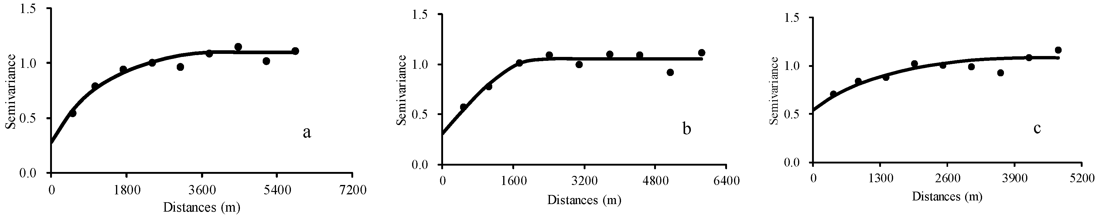
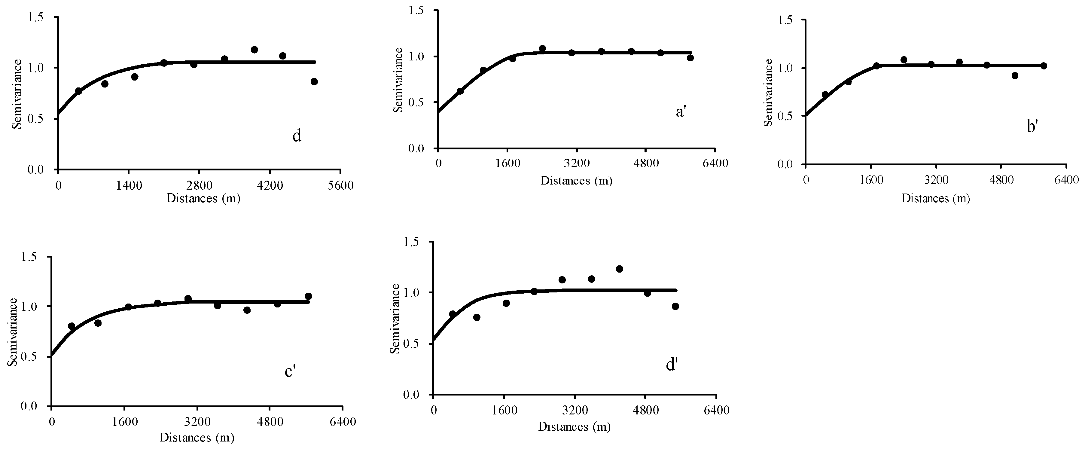
3.2. Geostatistical Analysis of SOC Contents

Taking the v₁, v₂, v₃, and v₄, whose VMR values were the closest to the mean VMR values of the corresponding discretization levels as the examples, the semivariogram models and their parameters of the original SOC data and the residual data (Formula 5) are shown in the

Table 3. The semivariance model and the parameters for the original data and the residuals of the SOC contents.

Method	Discretization	Distribution	Model	C0	Sill	C/Sill	Range (m)	R2
Ordinary Kriging (OK)	v1	Normal	Exponential	0.28	1.10	0.74	3480	0.94
	v2	Normal	Spherical	0.31	1.06	0.71	2190	0.82
	v3	Normal	Exponential	0.54	1.09	0.50	3870	0.75
	v4	Normal	Exponential	0.56	1.06	0.47	2430	0.58
Kriging with land use information (LuK)	v1	Normal	Spherical	0.40	1.04	0.62	2170	0.96
	v2	Normal	Spherical	0.51	1.03	0.50	2030	0.88
	v3	Normal	Exponential	0.52	1.05	0.50	2340	0.79
	v4	Normal	Exponential	0.54	1.02	0.47	1830	0.42

. The best-fitting models of the original SOC data were exponential, spherical, exponential, and exponential, respectively (Figure 3). The nugget (C₀) values were 0.28, 0.31, 0.54, and 0.56, and the Sill values were 1.10, 1.06, 1.09, and 1.06, while the corresponding ratios of C to Sill (i.e., C/Sill) were 0.74, 0.71, 0.50, and 0.47, respectively. Judging from the spatial autocorrelation degree, the original SOC data at various discretization levels all had a medium degree of spatial autocorrelation [35]. In terms of the SOC residual data, by removing the SOC mean value of the corresponding land use pattern, the best-fitting models at the v₁ and v₂ levels were spherical models, and those at the v₃ and v₄ levels were exponential models. Their nugget (C₀) values were 0.40, 0.51, 0.52, and 0.54, while the corresponding Sill values were 1.04, 1.03, 1.05, and 1.02, respectively. It can be seen that the SOC residual data as well as the original SOC data all had a medium degree of spatial autocorrelation at the four discretization levels. Moreover, the C/Sill ratios of the original SOC data and the SOC residual data both decreased with an increase in VRM values. This indicates that the structural factors that influence the SOC’s variability in SOC decreased, while the random factors caused by unknown conditions increased. So, the uncertainty of the predicted results in terms of SOC variability will consequently rise with an increase in sample discretization. Furthermore, the determination coefficients (R²) of the model fitting also decreased, which illustrated that the fitting model is more unfavorable for obtaining the SOC variability information as the discretization level increases.

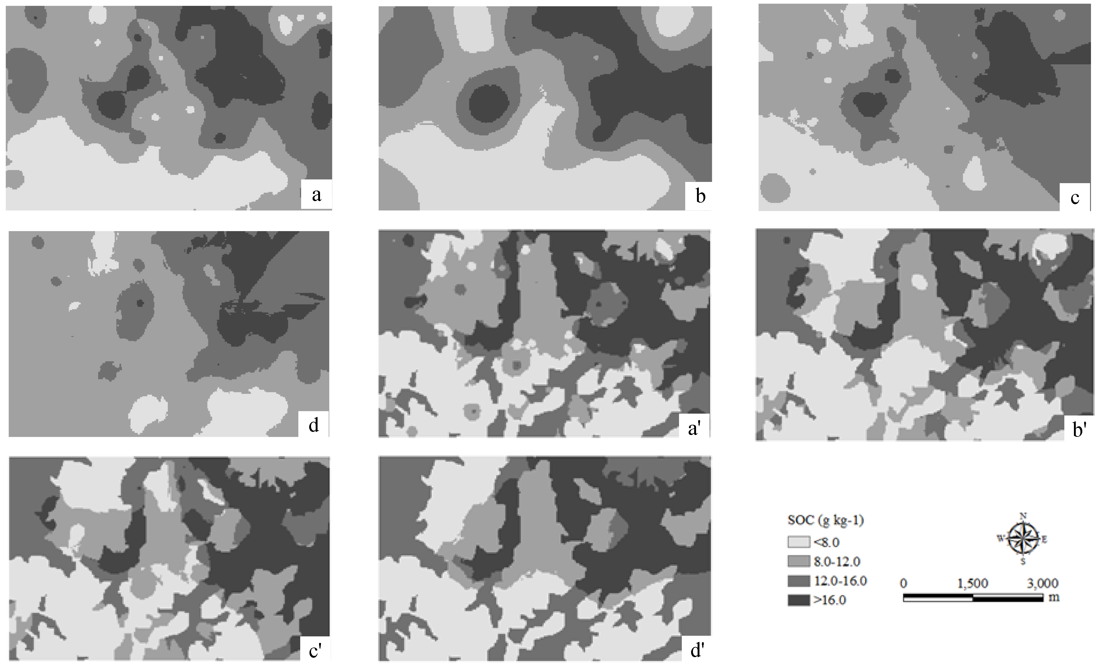
3.3. Interpolation Contours of SOC Content at the Various Sample Discretization Levels

The interpolation maps of the SOC contents obtained by two methods at four discretization levels (also taking v₁–v₄ as examples) are shown in Figure 4. The distributions of SOC at v₁–v₄ levels showed a similar trend to the SOC contents—they were high in the northeast area and low in the southwest area. The SOC content in most of the northeast area exceeded 16.0 g kg⁻¹, and that in the southwest area was less than 8.0 g kg⁻¹. The areas with high SOC content were mainly occupied by paddy fields, while those with lower content were mainly occupied by dry land and sparse forestland. Owing to the relatively high yield of agricultural output in paddy fields, their SOC content was high with more fertilizer input and plenty of straw being returned to the fields. Contrarily, the SOC content of dry land was low because it had less fertilizer input, and its soil moisture condition was not conducive to SOC accumulation. Most forestland in the study area had been restored from slope farmland after 2000, and the vegetation was still sparse and the growth status of understory shrubs was not as good as that of traditional forests; therefore, its SOC content was only slightly higher than that of dry land.

Furthermore, it was found that there were great differences in the detailed characteristics of SOC distribution at different discretization levels. Firstly, the characteristics of SOC in some areas obtained by the two Kriging methods were quite different because of their different interpolation principles. As the OK method did not consider the differences in SOC content between land use patterns, the interpolation maps of SOC obtained by OK were continuous and regular. The relative differences in SOC contents between land use patterns were considered in the LuK method, and the SOC distribution obtained by LuK was consistent with the spatial distribution patterns of land use. Thus, LuK can better reveal the true distribution of SOC in Yujiang County. Secondly, the SOC distribution details in some local areas obtained by the same prediction method were also quite different at the various discretization levels. The distribution patterns of SOC content and the occupied areas of the statistical subsections were also different at the various levels; they were closely related to the respective sampling points’ spatial distribution characteristics.

3.4. Uncertainty Evaluation of Spatial Interpolation at Various Discretization Levels

From the predicted mean MAE and RMSE values of three repetitions (Figure 5), the interpolation accuracies of LuK were higher than those of OK at four discretization levels. In addition, the predicted MAE and RMSE values obtained from the two methods both improved with increasing discretization. The MAEs of the OK method were 4.47, 4.65, 5.03, and 5.46 g kg⁻¹ at the levels of V₁–V₄, respectively, and the corresponding RMSEs were 5.10, 5.52, 5.70, and 6.12 g kg⁻¹, respectively. Compared with the errors at the V₁ level (VMR = 0.12), the MAE and RMSE values at the V₄ level (VMR = 2.17) increased by 22.1 and 20.0%, respectively. Similarly, the MAEs based on LuK were 3.02, 3.10, 3.24, and 3.54 g kg⁻¹, and the RMSEs were 3.61, 3.79, 3.98, and 4.02 g kg⁻¹ at the V₁–V₄ levels, respectively. Compared with the V₁ level, the predicted MAE and RMSE values at the V₄ level increased by 17.2 and 11.4%, respectively. The comparison results showed that the spatial discretization level of soil sampling points has an important influence on the uncertainty in SOC spatial interpolation.

The distribution maps of the predicted absolute errors (AE) obtained through the evenly-distributed verification points at the various discretization levels are shown in Figure 6. As seen from the figure, firstly, there are more darker grids in Figure 6a–d than in a’ to d’, which indicates that the number of integrated prediction errors in OK was higher than in LuK at all discretization levels. Secondly, with increasing sample discretization, the distribution of sampling points became increasingly uneven, and the grids with a high number of errors showed an increasing tendency. Then, the distributions of high error values were basically consistent with the sparse areas of sampling points, which indicated that the distribution of sampling points has a great influence on the distribution of the spatial prediction error.

4. Discussion

In this study, we studied the influence of the sample discretization level on revealing the spatial variability of SOC by Kriging methods. The results showed that the spatial prediction errors of SOC by the two Kriging methods both rose with an increase in the discretization levels. The predicted MAE values of SOC at the V₄ discretization level were 22.1% (OK) and 17.2% (LuK) higher than those at the V₁ level, and the corresponding RMSE values increased by 20% (OK) and 11.4% (LuK), respectively. This illustrates that the discretization level of sampling points is an important influencing factor, in addition to sampling point quantity, sampling point interval, and interpolation method selection. However, soil researchers have rarely considered the influence of the discretization level of soil sampling points when studying the spatial variability of regional SOC based on soil sampling. Actually, in soil survey sampling, the sampling points are usually not uniformly distributed in stratified sampling designs [14], strip sampling designs [36], and even in some simple random sampling designs [37]. If the sampling points from these designs have high discretization levels, the interpolated errors with regional SOC distribution maps will be improved to a certain extent. Therefore, it is necessary to know that the spatial distribution characteristics of the sampling points may affect the interpolation accuracy when the Kriging method is utilized for spatial interpolation. In order to reduce the uncertainty of SOC spatial interpolation, the uniform distribution points with a low discretization level should be used as far as possible for the interpolation using Kriging methods.

From the results of this study, it is known that the sample discretization level has an important influence on the interpolation accuracy of Kriging methods. Meanwhile, the interpolation accuracies of different Kriging methods had different responses to the variation in the sample discretization level. The comparative analysis showed that with an increase in discretization, the interpolation error of the OK method increased more than that of the LuK method. It was shown that the sample discretization level has a large influence on the accuracy of the OK method, while it has a relatively small influence on that of LuK. That is, OK is more sensitive to the sample discretization level than the LuK method in regional SOC interpolation. Because the large differences in SOC content among different land use patterns are not considered, the OK method has a large prediction error with a strong smoothing effect [38], which can reduce the high SOC content values and increase the low values for the unknown points. In the current study, with an increase in the sample discretization level, the sampling points in some local areas became relatively scarce. As a result, the uncertainty of SOC interpolation in these local areas was largely increased, and then the prediction accuracy of whole research area was reduced. Contrastively, LuK method reduced the smoothness effect by eliminating the mean value of SOC content of each land use pattern. With an increase in the discretization level of sampling points, the sampling points will also become sparse in some local areas, but the prediction error will not be too high, as the SOC content of every unknown point is composed of two parts: the residual value and the mean value of the corresponding land use (Equation (6)). Thus, the disadvantageous influence of having a large sample discretization level was alleviated in the Kriging interpolation of regional SOC. It can be seen that the LuK method, which incorporates land use information, not only had a higher SOC spatial prediction accuracy than the OK method, but also, its prediction accuracy reduction was slower than OK with an increase in sample discretization.

In this study, the influence of sampling point discretization on revealing the regional SOC variability was studied with two Kriging methods. The general variation in the regularity of interpolation accuracy with the variation in sample discretization was obtained at four sample discretization levels. The mechanisms and quantitative characterization of the influence of sampling point discretization on other spatial interpolation methods (e.g., other Kriging methods not mentioned in this study, the polygon-based method, and the polynomial method) require further research to be confirmed. In addition, the SOC, as an important soil property, was taken as the research example in this study. However, for other soil properties, which also can be considered to be regionalized variables, the relationship between the varying sampling points’ discretization levels and spatial interpolation accuracies also needs to be further clarified.

5. Conclusions

Here, we comparatively analyzed the influence of sampling point discretization on the SOC variability using two Kriging methods at four discretization levels in the red soil region, China. We found that the interpolation uncertainty of SOC both rose with an increase in the discretization level for both methods. This result shows that the spatial uniform distribution of soil sampling points is beneficial to the Kriging interpolation and the revealing of the regional SOC variability. The uneven distributed sampling points with large discretization are an important error source in Kriging interpolation. Furthermore, the interpolation uncertainty of OK was shown to be more sensitive than LuK to the variation in discretization level. This shows that different Kriging methods have different responses to sampling point discretization owing to their specific estimation principles. These results are of significance to the high-precision revealing of soil properties and the sampling theory of regional soil surveys.

References

1. Lal, R. Soil carbon sequestration to mitigate climate change. Geoderma 2004, 123, 1–22. [Google Scholar] [CrossRef]
2. Jones, C.; Mcconnell, C.; Coleman, K.; Cox, P.; Falloon, P.; Jenkinson, D. Global climate change and soil carbon stocks; predictions from two contrasting models for the turnover of organic carbon in soil. Glob. Chang. Biol. 2010, 11, 154–166. [Google Scholar] [CrossRef]
3. Wang, S.; Zhuang, Q.; Wang, Q.; Jin, X.; Han, C. Mapping stocks of soil organic carbon and soil total nitrogen in liaoning province of china. Geoderma 2017, 305, 250–263. [Google Scholar] [CrossRef]
4. Zeng, H.; Xu, H.; Liu, Z.; Huang, X.; Xiao, S. Variability of soil organic carbon and factors affecting it in residential lands in a rapidly urbanizing area: A case study of nantai island of fuzhou city, china. Acta Ecol. Sin. 2018, 38, 1427–1435. (In Chinese) [Google Scholar] [CrossRef]
5. Zhang, H.; Wu, P.; Yin, A.; Yang, X.; Zhang, M.; Gao, C. Prediction of soil organic carbon in an intensively managed reclamation zone of eastern china: A comparison of multiple linear regressions and the random forest model. Sci. Total Environ. 2017, 592, 704–713. [Google Scholar] [CrossRef] [PubMed]
6. Hounkpatin, O.; Hipt, F.; Bossa, A.; Welp, G.; Amelung, W. Soil organic carbon stocks and their determining factors in the dano catchment (southwest burkina faso). Catena 2018, 166, 298–309. [Google Scholar] [CrossRef]
7. Zhang, Z.; Yu, D.; Shi, X.; Weindorf, D.; Wang, X.; Tan, M. Effect of sampling classification patterns on SOC variability in the red soil region, China. Soil Till. Res. 2010, 110, 2–7. [Google Scholar] [CrossRef]
8. Hedley, C.; Payton, I.; Lynn, I.; Carrick, S.; Webb, T.; Mcneill, S. Random sampling of stony and non-stony soils for testing a national soil carbon monitoring system. Soil Res. 2012, 50, 18–29. [Google Scholar] [CrossRef]
9. Sankey, J.; Brown, D.; Bernard, M.; Lawrence, R. Comparing local vs. global visible and near-infrared (VisNIR) diffuse reflectance spectroscopy (DRS) calibrations for the prediction of soil clay, organic C and inorganic C. Geoderma 2008, 148, 149–158. [Google Scholar] [CrossRef] [Green Version]
10. Jiao, J.; Yang, L.; Wu, J.; Wang, H.; Li, H.; Ellis, E. Land use and soil organic carbon in China’s village landscapes. Pedosphere 2010, 20, 1–14. [Google Scholar] [CrossRef]
11. Zhang, S.; Xu, M.; Zhang, Z.; Li, B.; Na, A.; University, F. Methods of Sampling Soil Organic Carbon in Farmlands with Different Landform Types on the Loess Plateau. J. Nat. Resour. 2018, 33, 634–643. (In Chinese) [Google Scholar] [CrossRef]
12. Bhatta, K.; Chaudhary, R.; Vetaas, O. A comparison of systematic versus stratified-random sampling design for gradient analyses: A case study in subalpine Himalaya, Nepal. Phytocoenologia 2012, 42, 191–202. [Google Scholar] [CrossRef]
13. Liu, D.; Wang, Z.; Zhang, B.; Song, K.; Li, X.; Li, J. Spatial distribution of soil organic carbon and analysis of related factors in croplands of the black soil region, Northe’ast China. Agric. Ecosyst. Environ. 2006, 113, 73–81. [Google Scholar] [CrossRef]
14. Huang, B.; Sun, W.; Zhao, Y.; Zhu, J.; Yang, R.; Zou, Z.; Ding, F.; Su, J. Temporal and spatial variability of soil organic matter and total nitrogen in an agricultural ecosystem as affected by farming practices. Geoderma 2007, 139, 336–345. [Google Scholar] [CrossRef]
15. Liu, N.; Wang, Y.; Wang, Y.; Zhao, Z.; Zhao, Y. Tree species composition rather than biodiversity impacts forest soil organic carbon of Three Gorges, southwestern China. Nat. Conserv. 2018, 14, 7–24. [Google Scholar] [CrossRef]
16. Frogbrook, Z.; Bell, J.; Bradley, R.; Evans, C.; Lark, R.; Reynolds, B.; Smith, P.; Towers, W. Quantifying terrestrial carbon stocks: Examining the spatial variation in two upland areas in the UK and a comparison to mapped estimates of soil carbon. Soil Use Manag. 2009, 25, 320–332. [Google Scholar] [CrossRef]
17. Yu, D.; Zhang, Z.; Yang, H.; Shi, X.; Tan, M.; Sun, W.; Wang, H. Effect of sampling density on detecting the temporal evolution of soil organic carbon in hilly red soil region of South China. Pedosphere 2011, 21, 207–213. [Google Scholar] [CrossRef]
18. Zhang, Z.; Yu, D.; Wang, X.; Pan, Y.; Zhang, G.; Shi, X. Influence of the Selection of Interpolation Method on Revealing Soil Organic Carbon Variability in the Red Soil Region, China. Sustainability 2018, 10, 2290. [Google Scholar] [CrossRef]
19. Zhao, Y.; Shi, X.; Weindorf, D.; Yu, D.; Sun, W.; Wang, H. Map scale effects on soil organic carbon stock estimation in North China. Soil Sci. Soc. Am. J. 2006, 70, 1377–1386. [Google Scholar] [CrossRef]
20. Kumar, S.; Lal, R.; Liu, D. A geographically weighted regression kriging approach for mapping soil organic carbon stock. Geoderma 2012, 189–190, 627–634. [Google Scholar] [CrossRef]
21. Kerry, R.; Goovaerts, P.; Rawlins, B.; Marchant, B. Disaggregation of legacy soil data using area to point kriging for mapping soil organic carbon at the regional scale. Geoderma 2012, 170, 347–358. [Google Scholar] [CrossRef] [PubMed] [Green Version]
22. Wang, S.; Zhuang, Q.; Jia, S.; Jin, X.; Wang, Q. Spatial variations of soil organic carbon stocks in a coastal hilly area of China. Geoderma 2018, 314, 8–19. [Google Scholar] [CrossRef]
23. Dai, W.; Zhao, K.; Fu, W.; Jiang, P.; Li, Y.; Zhang, C.; Gielen, G.; Gong, X.; Li, Y.; Wang, H.; et al. Spatial variation of organic carbon density in topsoils of a typical subtropical forest, southeastern China. Catena 2018, 167, 181–189. [Google Scholar] [CrossRef]
24. Chai, X.; Shen, C.; Yuan, X.; Huang, Y. Spatial prediction of soil organic matter in the presence of different external trends with REML-EBLUP. Geoderma 2008, 148, 159–166. [Google Scholar] [CrossRef]
25. Liu, T.; Juang, K.; Lee, D. Interpolating soil properties using kriging combined with categorical information of soil maps. Soil Sci. Soc. Am. J. 2006, 70, 1200–1209. [Google Scholar] [CrossRef]
26. Kumar, N.; Velmurugan, A.; Hamm, N.; Dadhwal, V. Geospatial Mapping of Soil Organic Carbon Using Regression Kriging and Remote Sensing. J. Indian Soc. Remote 2018, 3, 1–12. [Google Scholar] [CrossRef]
27. Wang, J.; Liao, Y.; Liu, X. Course of Spatial Data Analysis, 1st ed.; Science and Technology Press: Beijing, China, 2010; pp. 74–75. ISBN 978-7-03-026605-7. [Google Scholar]
28. IUSS Working Group WRB. World Reference Base for Soil Resources 2006; World Soil Resources Reports No. 103; UN Food and Agriculture Organization: Rome, Italy, 2006; pp. 71–72. [Google Scholar]
29. Soil Survey Office of Yujiang County. Soil Species of Yujiang County; Science and Technology Press: Beijing, China, 1986.
30. Zhang, Z.; Yu, D.; Shi, X.; Wang, N.; Zhang, G. Priority selection rating of sampling density and interpolation method for detecting the spatial variability of soil organic carbon in China. Environ. Earth Sci. 2015, 73, 2287–2297. [Google Scholar] [CrossRef]
31. Nelson, D.W.; Sommers, L.E. Total carbon, organic carbon, and organic matter. In Methods of Soil Analysis, Part2-Chemical and Microbiological Properties; Page, A.L., Miller, R.H., Keeney, D.R., Eds.; ASA-SSSA: Madison, WI, USA, 1982; pp. 539–594. [Google Scholar]
32. Wong, D.W.S.; Lee, J. Statistical Analysis of Geographic Information with ArcView GIS and ArcGIS; Wiley: Hoboken, NJ, USA, 2005; pp. 218–279. [Google Scholar]
33. Zhang, Z.; Shi, X.; Yu, D.; Weindorf, D.; Sun, W.; Wang, H.; Zhao, Y. Effect of prediction methods on detecting the temporal evolution of soil organic carbon in hilly red soil region of South China. Environ. Earth Sci. 2011, 64, 319–328. [Google Scholar] [CrossRef]
34. Chaplot, V.; Bouahom, B.; Valentin, C. Soil organic carbon stocks in Laos: Spatial variations and controlling factors. Glob. Chang. Biol. 2010, 16, 1380–1393. [Google Scholar] [CrossRef]
35. Qiu, J.; Wang, L.; Li, H.; Tang, H.; Li, C.; Ranst, E. Modeling the Impacts of soil organic carbon content of croplands on crop yields in China. Agric. Sci. China 2009, 8, 464–471. [Google Scholar] [CrossRef]
36. Emery, X. Uncertainty modeling and spatial prediction by multi-gaussian kriging: Accounting for an unknown mean value. Comput. Geosci. 2008, 34, 1431–1442. [Google Scholar] [CrossRef]
37. Cochran, W.G. Sampling Techniques; John Wiley & Sons: Hoboken, NJ, USA, 2007. [Google Scholar]
38. Kerry, R.; Oliver, M. Determining nugget: Sill ratios of standardized variograms from aerial photographs to krige sparse soil data. Precis. Agric. 2008, 9, 33–56. [Google Scholar] [CrossRef]
Figure 1. Location of the study area and the distribution of soil sampling points.
Sustainability 10 03603 g001
Figure 2. Distribution of resampling points for the four discretization levels ((a,b,c), and (d) correspond to the discretization of v1, v2, v3, and v4).
Sustainability 10 03603 g002
Figure 3. The semivariance of SOC contents (ad) and residual data (a’d’) at the different discretization of v1, v2, v3, and v4, respectively.
Sustainability 10 03603 g003aSustainability 10 03603 g003b
Figure 4. Spatial distribution of SOC content based on various sample discretization levels ((ad) and (a’d’) were at the discretization levels of v1v4, respectively).
Sustainability 10 03603 g004
Figure 5. Interpolation MAE (a) and RMSE (b) of the SOC content at the various discretization levels (a–d represent the mean interpolation errors of three repetitions at the V1V4 levels, respectively).
Sustainability 10 03603 g005
Figure 6. Distribution of the interpolation errors with the validation points at the various discretization levels ((ad) and (a’d’) represent the discretization levels of v1v4, respectively).
Sustainability 10 03603 g006