Article

Vaguely Right or Exactly Wrong: Measuring the (Spatial) Distribution of Land Resources, Income and Wealth in Rural Ethiopia

1
Human Geography & Planning, Faculty of Geosciences, Utrecht University, Utrecht 3508TC, The Netherlands
2
Netherlands Environmental Assessment Agency, The Hague 2500GH, The Netherlands
3
The Horn Economic and Social Policy Institute, Kirkos Sub City 1250, Ethiopia
*
Author to whom correspondence should be addressed.
Sustainability 2017, 9(6), 962; https://doi.org/10.3390/su9060962
Submission received: 10 March 2017 / Revised: 30 May 2017 / Accepted: 1 June 2017 / Published: 6 June 2017
(This article belongs to the Section Economic and Business Aspects of Sustainability)

Abstract

:
Land ties people to specific localities featuring different levels of accessibility and natural endowments; it is therefore related in various ways to matters of inequality. Drawing from economics and human geography, we explore the multifaceted and complex nature of inequality. Our case study takes place in rural Tigray, Ethiopia. Quantitative data analysis is used to reveal (spatial) income distribution patterns between statistically representative population groups. Qualitative data are then used to describe the productive activities of these groups, their respective processes of material asset accumulation or losses, and how their economic activities are affected by location. The paper concludes that, where measures of the distribution of income falls short, we require other tools that will help us reveal patterns: (1) of material wealth distribution; (2) of control over production; and (3) of the unaccounted value created within the household or derived from the natural environment.

1. Introduction

Land is the primary means of production in the global South. Output produced in excess of the needs of the household is sold, and if the family cannot perform all the required work, it could become a net employer. Subsistence farmers, on the other hand, could become net buyers of output; and family labour in excess of what is needed on the home plot could be sold (we draw from the insight that the household as a unit of analysis includes producer, consumer, employer and labourer activities [1]). Land allows families to potentially increase income and reduce spending. It therefore represents the main asset upon which they can accumulate further wealth for themselves and for their children, such as livestock, irrigation systems, farming tools, means of transportation, or additional land. The capacity of households to manage their properties productively is therefore a key factor in the generation of economic inequalities. Hence, development research and policy often ask whether producer–labourer households will endure as a category, or whether they will over time tend to differentiate in landless workers and commercial farmers, and, if so, which category will dominate [1].
Land is not only a means of production; it also ties people to specific localities. Ethiopia is one of the few countries in Africa that has not made significant changes in its land policy since 1975 when tenant–landlord relationships were abolished. Landownership remains vested in the state and farmers hold usufruct land rights through state-mandated peasant associations, subject to proof of permanent residence, and subject to on-going active land cultivation. These rights are inheritable and can be temporarily transferred to others through rental agreements, but the land itself cannot be sold [2,3]. This system is fiercely criticised for the lack of tenure security, the resulting low productivity it creates, the discriminatory practices in land distribution and the discouraging effect on geographical mobility. Others counter that private ownership would lead to a concentration of land in the hands of more competitive or more powerful households, resulting in the eviction of a large underemployed and underpaid labour force (for an overview of the debate, see [3,4]).
The issue for this paper is that a rural population that is geographically, economically and constitutionally tied to the land is also more confined to the natural endowment of its direct surroundings, which may or may not include water resources, healthy soils, free grazing space, forested landscapes, and so on. These localities are also “endowed” with different levels of accessibility to other localities of economic importance, such as labour, food and livestock markets, extension services or business investment opportunities. The fact that most households are likely to have stayed in the same place since the last land redistribution of 1991 makes it possible to highlight the effects of an uneven proximity to natural and economic resources, and to disregard displacement or migration of entire family units. While some family members may have migrated, household heads risk losing land rights without proof of permanent residency in the specific locality [3].
While the land policy has a geographically confining effect, rural livelihoods are by no means static as manifested by the everyday flows of people and their commodities. There is a general expectation that these flows will be further stimulated through investments in roads, transportation and telecommunication. However, it is also conceivable that financial, cultural or environmental barriers could bring about an uneven rise in mobility and accessibility for different social groups: after all, “one person’s speed is another person’s slowness” [5] (p. 21). For example, the quickest or better informed producer will get to the most profitable markets first, and sell their product at a higher price, until such point when other producers follow and prices fall. Meanwhile, the poorer consumer whose action radius is generally shorter does not have the same leeway to choose where to buy his or her necessities. Although such disparities would also have existed before the infrastructure investments, they may be either reduced or catalysed by the increased scale and speed of connectivity.
Factors explaining wealth distribution and accumulation over time therefore include: inheritance, local natural endowment, accessibility, scale, speed, but also chance, status, political power and so on. As a consequence of these complexities, economists found it more practical to measure inequalities in income or spending rather than to disentangle wealth in its various ingredients and proportions—let alone its distribution [6,7]. Inequality is generally quantified by slicing a population into income or expenditure segments. For example, a rough indication of the trend in Ethiopia is provided by the consumption gap, which increased from 0.28 to 0.30 (Gini coefficient) in the period 2000–2011 [8].
Income or spending metrics fail to reveal how individuals and households participate in the economy. A step in the right direction is to distinguish between the income generated from capital and the income generated from labour [9]. Recent evidence from different parts of the world reveals that the gap in the former is wider than the gap in the latter [9,10,11,12]. It is assumed that the pattern of distribution of income from capital largely reflects the distribution of material assets between households. This leads to the following questions: to what extent is this reflection accurate? What does income from capital as a proxy for material wealth hide and reveal?
The paper’s objectives are threefold:
(1)
First, we present evidence of the income gaps for rural Tigray, Ethiopia. Based on survey data, we reveal different income categories and distinguish between their sources of income (labour and capital).
(2)
The second objective is to explore the spatial dimensions of inequality. Survey data are used to reveal correlations between income and access to economic resources. Proximity to natural resources, on the other hand, is based on qualitative accounts of the natural endowments present in the different localities.
(3)
The third objective is to contribute to the broader question of the discrepancy between income and wealth inequalities. For this, we rely on qualitative descriptions of household activities, drawing from wealth ranking workshops and in-depth interviews. Our paper ends with some recommendations for a research and policy agenda.

2. Methodology

The nature of the topic calls for a mixed method approach drawing from economics and (human) geography:
(1)
We rely on quantitative data from a household survey to describe patterns of income distribution and to distinguish between income from capital and income from labour. The sample is distributed over four geographic localities featuring different productive activities.
(2)
We explore proximity to economic and natural resources as two possible spatial explanations of inequality:
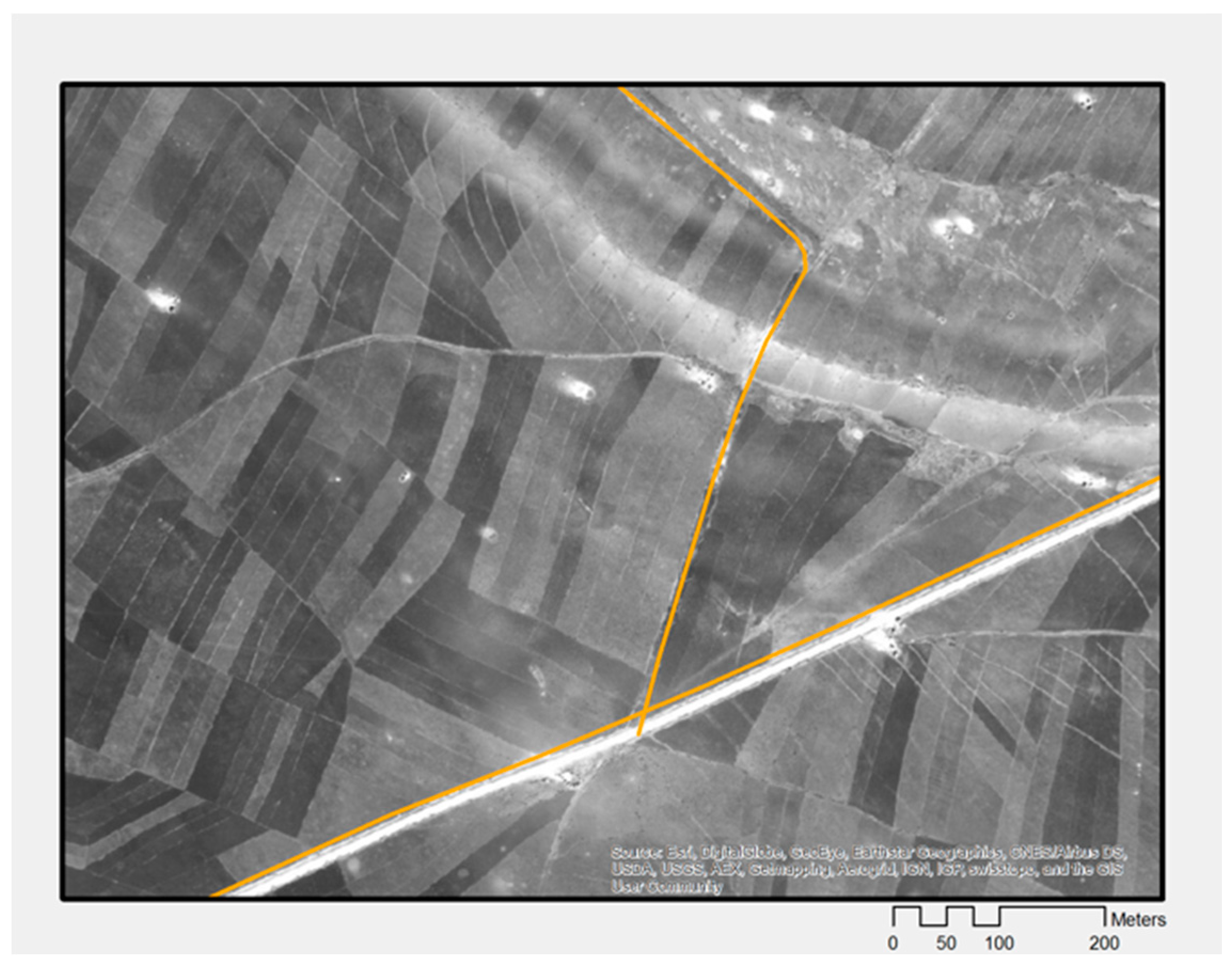
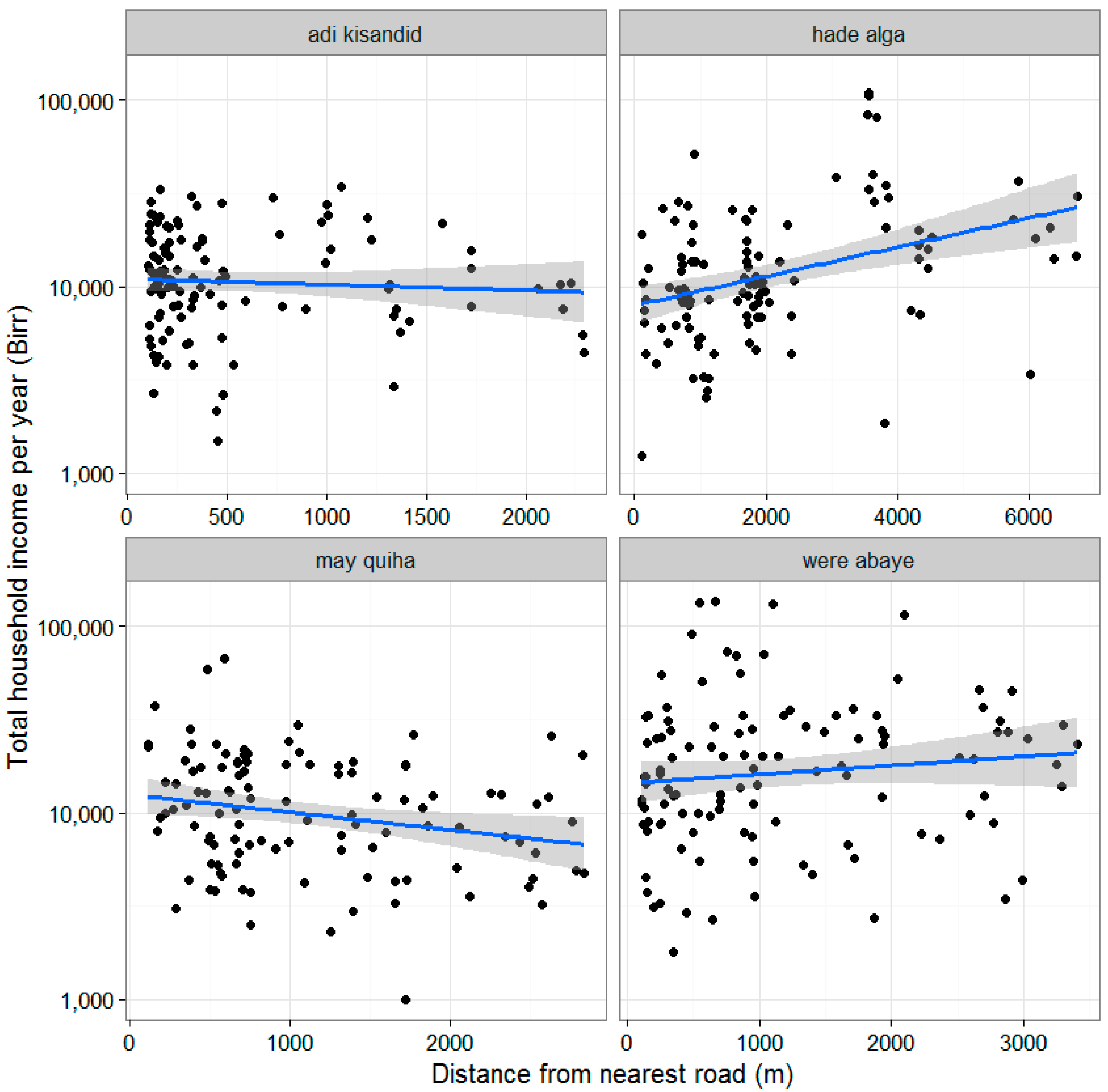
  • The effect of proximity to economic resources is studied quantitatively (the household survey entries were linked to GPS coordinates), based on correlations between income and distance to the nearest road, which is used as a proxy for access to economic resources.
  • In the absence of resource maps, the effect of proximity to natural resources on the spatial distribution of income is studied qualitatively based on semi-structured interview data.
(3)
Finally, semi-quantitative and qualitative data (from wealth ranking workshops and in-depth interviews, respectively) were collected to reveal patterns of material wealth distribution, and to reflect on possible discrepancies with income distribution statistics.
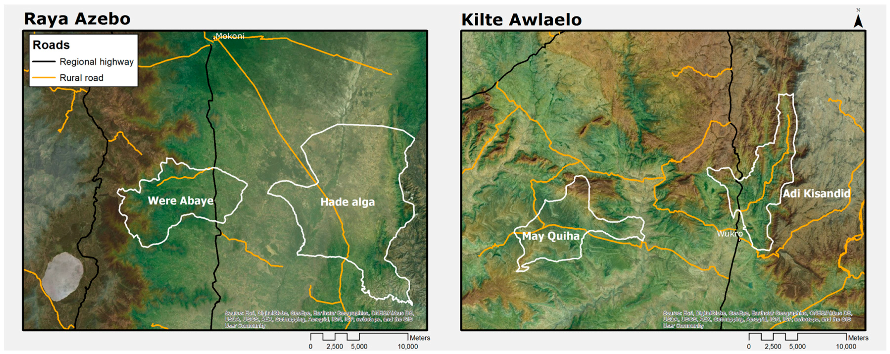
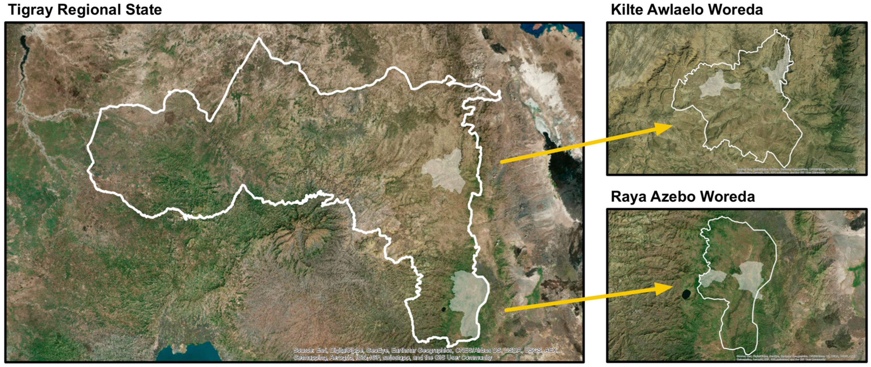
These activities were undertaken in the context of a two and a half year research programme aimed at investigating the (in)direct effects of rural road developments on productive employment. These developments are driven by the widespread assumption that the lack of roads is a major impediment to productivity. However, there is surprisingly little rigorous, empirical research dealing with the multiple effects on mobility, accessibility and livelihoods, as well as with the distribution of these effects.

2.1. Study Sites

To account for the role of geographical context in (income) distribution, we selected two woredas (or districts, the second administrative units above the tabia) with diverse topographic and economic characteristics, namely Raya Azebo and Kilte Awlaelo in Tigray regional state in northern Ethiopia (see maps in Figure 1 and Figure 2). Kilte Awlaelo in Eastern Tigray (with Wukro as the main woreda centre) is situated at higher altitude, features mountainous terrain and is generally developed for commercial cropping. Raya Azebo in Southern Tigray (with Mohoni as the main woreda centre) is lower, more arid and includes pastoralist activities. Two tabias (the smallest units of local government in rural communities in Tigray) were selected in each woreda:
  • In Kilte Awlaelo woreda: Adi Kisandid tabia (mountainous terrain, little pastoralism, mostly commercial cropping, intensively irrigated, rural road directly connected to a regional highway) and May Quiha tabia (flat terrain, some pastoralism, mostly rainfed agriculture, rural road indirectly connected to a regional highway).
  • In Raya Azebo woreda: Were Abaye tabia (mountainous terrain, relatively less pastoralism, mostly commercial cropping, intensively irrigated, rural road directly connected to a regional highway) and Hade Alga (flat terrain, some pastoralism, mostly rainfed agriculture, rural road indirectly connected to a regional highway).
These tabias are representative of most other tabias in terms of their connectivity and distance to localities of economic importance through a network of rural roads and regional highways. We based our selection on a range of criteria, including: (1) All tabias in the region are connected to the regional town, either directly through a tabia-to-woreda road, or indirectly through a tabia-to-tabia road that is linked to a tabia-to-woreda road. Both direct and indirect road connections were selected. (2) Tabias with diverse topographies were selected (flat and mountainous). (3) Tabias with different productive activities were selected (cropping or mixed cropping-pastoralism, which are the dominant economic activities). Our wider research programme also selected these sites based on the age of establishment of a rural road with the aim to explore temporal differences in road impacts, but that is not the focus of this paper. Here, we merely use roads as a proxy for access to economic resources outside of the tabia.
The selected woredas score above the Tigray average in terms of total non-crop income. (Non-crop income was estimated at 3415.63 birr/year in Kilte Awlaelo and 4239.45 in Raya Azebo for a 3159.82 average in Tigray. An important contribution to this difference is the relatively high sales of animal products and livestock [13].) This bias could imply a wider bandwidth between high- and low-income households in our sample. It could also imply that the lower incomes in our sample are relatively higher than in other woredas.

2.2. Income Data Collection and Analysis

Our analysis draws from a 2015 survey undertaken in rural Tigray, Ethiopia. A total of 529 sample households were selected from the four study tabias. With an average of 1683 households per tabia in our study sites (based on [14]), we covered about 8% of all households. Sample households were distributed proportionately to each tabia. In each tabia, sample households were also proportionately distributed to each sub-village locally called kushet (a tabia consists of three to four kushets). Lists of households were obtained from each kushet and simple systematic sampling was used to select households at regular intervals with a random start.
A multi-purpose questionnaire was used to gather information about demographics, mobility, activities and income. In this paper, we focus on the income data and the survey allows us to distinguish between the following sources of (non-)farm income:
(1)
Income from capital, which includes earnings or revenue from:
  • non-permanent crop harvest
  • trees or permanent crops and/or fruits from the trees
  • livestock products
  • own business activities
(2)
Income from wages, which includes:
  • wages from employment
  • transfer (aid) income (Transfer income in rural Tigray is earned through programmes such as food-for-work, cash-for-work, employment generation schemes and employment-based safety nets. The Productive Safety Net Programme, for example, has employed the rural poor in building roads and other infrastructure [8].)
  • remittance income (We assume that the income earned by migrants is mainly from formal and informal wages, and not from capital. This assumption is warranted, considering evidence from Tigray that most migrants earn income illegally [15] and are therefore unlikely to have been able to invest in capital.)
The dataset included a question about other non-farm income, but we excluded this indicator as only four respondents reported on another source, of which only two have specified the source.
Ten enumerators were trained and a pilot test was undertaken. There was regular supervision during the survey fieldwork and questionnaire forms were checked on the spot for inconsistencies. After fieldwork, all forms were manually checked for completeness and data encoders were hired to complete data entry.
The data were analysed by aggregating the reported earning sources in the survey into two categories, i.e., income from capital and income from wages. The inequality between both sources is one that has deeply influenced the analysis of inequality in general [9]. We recalculated the production from non-permanent crops as income based on the combination of reported production and reported prices (this accounts for the fact that not all reported production is sold, but may also be consumed directly). Income from permanent crops, non-permanent crops, livestock products and business were aggregated as income from capital. Wage income, transfer income and remittance income were aggregated as income from wages. Wage income was reported both per month and per year. In a context of low rates of labour utilisation, we used yearly income. Four respondents did not mention any income and were excluded from the analysis. The distribution of total income was strongly left-skewed and we therefore chose to perform regressions and corrections on log-transformed data. This transformation resulted in better model fits and the residuals were more evenly spread.
We calculated the effects of a number of household characteristics on total income. Regression on total income of factors such as age of the head of household and level of education do not offer significant results at the p < 0.05 level. Household size on the other hand is a strong predictor for income (p < 0.001). It is often suggested that income should therefore be adjusted for household size in order to measure inequality in standards of living rather than in income as such [9] (adjusting or controlling for other variables isolates the relationship between just the two variables in question). However, such an adjustment is controversial: on the one hand, a five-person household might face a tighter budget constraint than a two-person household with matching income. On the other hand, children are often put to work at a very young age and can quickly become net producers. If changing family size is a factor of income growth (or decline), then to adjust for it removes a part of what is going on [16]. In this paper, we will refer to uncorrected reported income, unless mentioned otherwise.
For the analysis of inequality, a useful indicator of total wage inequality is the P90/P10 ratio, that is, the ratio of the lower limit of the tenth decile to the upper limit of the first decile. In other words, it indicates the cut-off points in income below 90 and above 10 per cent of all respondents. Other indicators such as the Gini coefficient or the Theil and Atkinson indices capture overall inequality of the distribution and not just the gap between the extreme deciles. Nevertheless, interdecile indicators such as P90/P10 are by far the simplest and most intuitive [9]. This indicator should not be confused with the D10/D1 ratio, that is, the ratio of the average wage of the tenth decile to that of the first decile, which is by definition always higher. The dataset was also aggregated into income groups. This was done in two ways: first, based on the deciles used by Piketty (2015) (D1 to D9 and then P90–P95 and P95–P100 to see a more fine-grained distribution of the tenth decile) and, second, based on the three categories suggested during the wealth ranking workshops (D1–D5, D6–D8 and D9–D10). Here, we assume that the distribution of income (from the survey) reflects the distribution of wealth (from the wealth ranking workshops), an assumption we will return to in the paper.
Average income level and proportion of income from different sources were calculated per income group. The P90/P10 interdecile ratios were calculated for the whole dataset and per tabia. The distribution of incomes was used to produce a tool for quick visual comparison of various PX/PX ratios.

2.3. Spatial Data Collection and Analysis

The survey interviews were geotagged, which allowed us to explore the spatial distribution of income inequality. More specifically, we looked at the correlations between income and proximity to economic resources.
The spatial analysis was performed by loading the survey data into ArcGIS based on the reported coordinates. Eleven respondents were excluded due to incorrectly entered coordinates (for example, one interview was reported many kilometres away from any of the tabias studied). A GIS layer of the location of the roads in 2015 was acquired from the Ethiopian Bureau of Construction, Road and Transport (BoCRT) and used to calculate the distance as the crow flies from each interview location to the nearest road. This road was either a rural road or a highway as shown in the earlier maps. The data were inspected by comparison with the Earth Systems Research Institute (ESRI) world imagery base maps and imprecisions were typically in the order of 10–20 m (see Figure 3). The imprecision was found to be no more than 40 m.
We calculated distance to the nearest tabia centre, as well as travel time to the nearest woreda administrative headquarters and economic centres. The latter was done by calculating the travel time through 100 × 100 m cells, assuming an average travelling speed of 20 km/h over roads and 5 km/h everywhere else.
All geographic analyses were extracted using ArcGIS, statistical analyses were performed in R. Regressions were performed using the standard linear model lm, aggregation was done with the use of the plyr package, visualisation with the help of the ggplot2 package. For calculation of the Gini coefficient, the ineq tool from the ineq package was used [17].
Alongside the quantitative spatial analysis of proximity to economic resources, we held 10 semi-structured interviews selected through random sampling. We relied on these interviews to cross-check our quantitative findings related to the spatial distribution of income and the importance of proximity to economic resources. These interviews revealed the importance of proximity to natural resources, which helps to explain some of the spatial patterns emerging from our data. The interviews lasted less than 20 min and probing continued until the information became repetitive.

2.4. Wealth Data Collection and Analysis

Our quantitative analysis of the income distribution patterns was further interpreted with qualitative data from workshops and interviews. The purpose was to expand on the issue of income versus wealth (as the survey dataset is limited to the former). We therefore distinguished wealth from the income it generates. The difference can be defined as such:
Wealth is a stock of assets, measured at a point in time, that is, cash in the bank, plus the market value of bonds, corporate shares, land, real estate, and consumer durables as of a given date. Income is the flow of earnings from these assets, plus the earnings of your own labour power (or human capital), between two dates, that is, over a period of time... Income and wealth are thus two different magnitudes, measured in different units, and distributed differently over the population”.
[7] (p. 304)
In each tabia, we conducted participatory wealth ranking workshops [18]. Through snowball sampling and with the assistance of local teachers and leaders, participants were selected from different kushets and socio-economic backgrounds—subsistence and surplus producers, landless labourers, mixed households, etc. Considering that 24% of rural households in Tigray are female-headed [13], our sample included the heads of household from both gender groups. During the sessions, participants categorised different wealth groups according to a list of indicators that they developed themselves. They then estimated the percentage of households in each wealth group. Our questions included:
  • What are the sources of wealth in this tabia? (e.g., agriculture, business, etc.)
  • What are the wealth indicators that tell households apart? (e.g., livestock, dwelling, etc.)
  • How many wealth groups do you perceive? (e.g., extremely poor, middle class, etc.)
  • Per indicator, how does one wealth group compare to the others? (e.g., four oxen for the rich)
  • Finally, how large is each wealth group (number of households) in this tabia?
Each workshop lasted about two hours. In all cases, three main wealth groups were identified, despite the presence of extreme outliers. In general, 50% of the households were said to be in the “poor” category, 30% in the “middle” and 20% in the “rich”. As there was no strict upholding of a definition of wealth during the workshops, participants also discussed food security and income, for example, but only in passing. The emphasis was on material wealth, which is not surprising considering the very low rates of saving (only the very rich were mentioned to have accumulated financial assets). Key indicators mentioned by the workshop participants included land, livestock, various crop types, cultivation and irrigation equipment, beehives, etc.
According to the participants in all four workshops, being “poor” in income also means being “poor” in wealth. Again, the question is to what extent is one a reflection of the other. As discussed in the introduction, the severity of income distribution is generally less severe than wealth distribution. We will come back to this core issue throughout the paper.
In each tabia, through snowball sampling, we then approached two households from each extreme wealth group (“rich” and “poor”) and one household in the “middle” group as an additional comparison. Initial information was gathered about two key indicators from the wealth ranking (hectares of land managed and livestock owned) in order to check the wealth categorisation. Through 20 in-depth and semi-structured interviews, we gathered information about the composition and age of the household members, about their major assets and the related productive activities.

3. Results

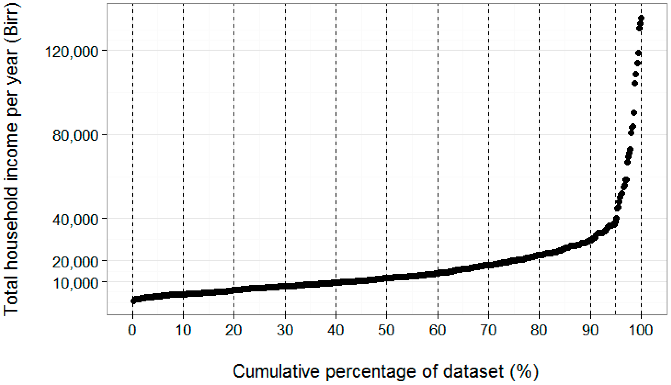
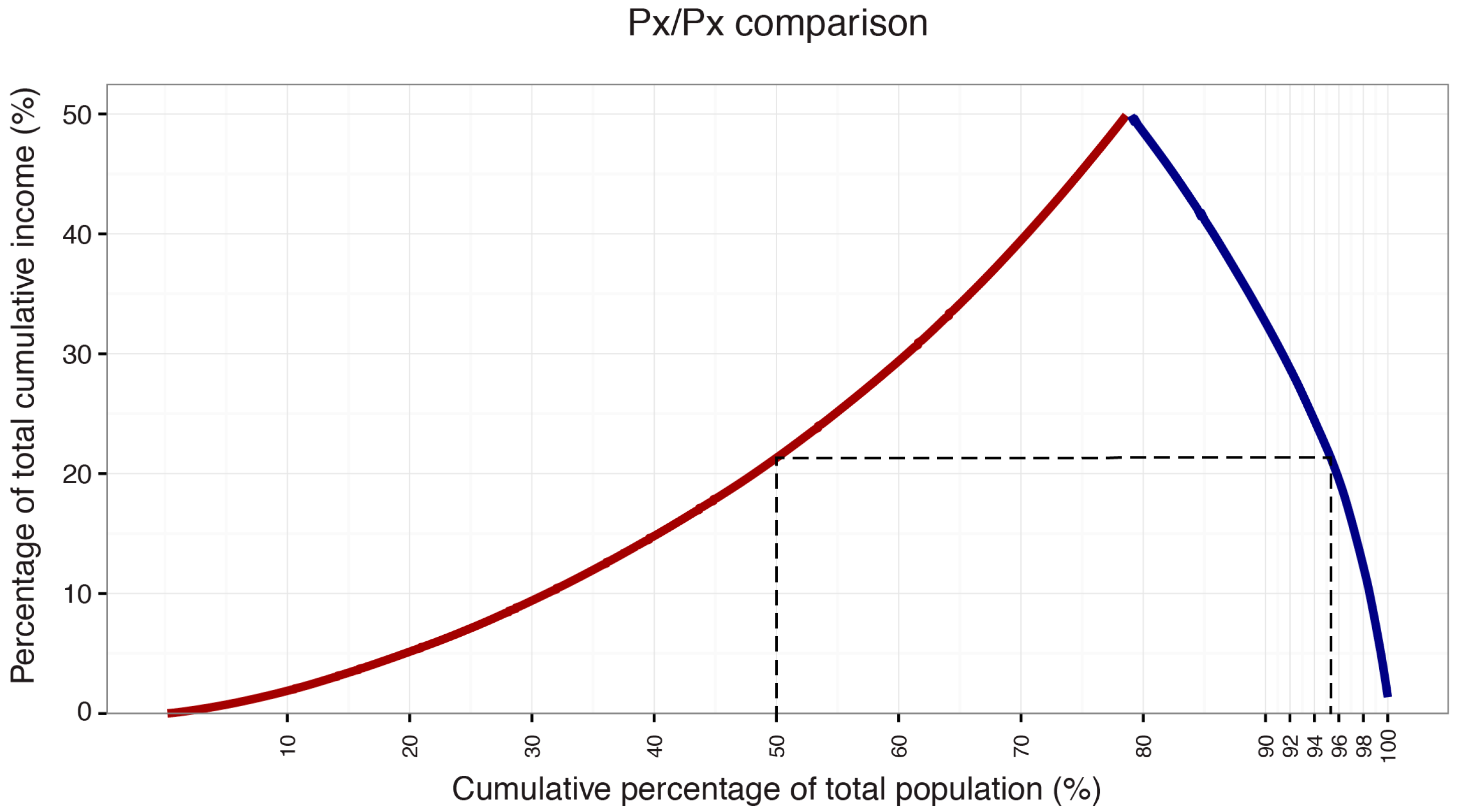
3.1. Income Distribution Patterns

Figure 4 shows total income (corrected for household size) as a function of the cumulative fraction of the population. At 0.5 on the x-axis, we see that 50% of the households earn a yearly income just above 10,000 birr, or $2032 (PPP). We used the $-birr conversion adjusted to purchasing power (PPP): 1 dollar (PPP) is equal to 4.92 birr [19]. More than 90% earn less than 30,000 birr per year, or $6097 (PPP). Several wealthy families earn around above 80,000 birr per year, or $16,260 (PPP). Converting the graph to a Lorentz curve gives us a GINI coefficient of 0.45. In a Lorentz curve, the x-axis shows the number of income recipients in terms of cumulative percentages, from lowest to highest income. The y-axis shows the percentage of total income. If there was perfect equality, the Lorenz curve would be a diagonal line that connects the bottom left to the top right corner of the graph. The GINI coefficient is equal to the area between the Lorenz curve and the diagonal divided by the total triangular area under the diagonal. With perfect equality, the GINI coefficient is 0. With perfect inequality, the GINI coefficient is 1 [7]. The inequality is higher in comparison to a GINI coefficient of 0.33 in 2010 for Ethiopia as a whole [19].
Based on the entire dataset, the P90/P10 ratio is 7.4. If one were to calculate the P90/P10 ratio for household income adjusted for household size, one would find a ratio of 7.0. It is lower than the unadjusted ratio, because larger households tend to earn higher incomes and adjusting for size would therefore reduce their income in a relative sense.
This aggregate P90/P10 ratio hides disparities between tabias. Indeed, the average household income in Were Abaye is almost double that of the other tabias (24,332 and 13,699 birr, respectively). From our initial site selection visits to the woreda, we know that this is quite exceptional. A significant number of farmers use irrigation which enables them to grow more than once in a year and benefit from perennial crops mainly khat (an amphetamine-like stimulant cash crop native to the Horn of Africa). Such a level of commercialisation cannot be found in other tabias in Raya Azebo or Kilte Awlaelo. The aggregate P90/P10 ratio also hides disparities within tabias, as shown in Table 1. Not only is Were Abaye generally better off, it is also more unequal in terms of its P90/P10 ratio. The table shows the lower limit of the tenth decile (P90) and therefore hides the income extremes that in this survey are as high as 135,550 and as low as 1600 birr per year (see Figure 4).
Based on the subjective categorisation suggested during the wealth ranking workshops, for the entire dataset (so to include all tabias), the better-off 20% earns on average 5.8 times more than the poorest 50% (see Table 2). We use the same categorisation by assuming that being “poor” in wealth also means being “poor” in income (even though both poverties are qualitatively different).
Approaching the question from both ends, so to speak, Figure 5 shows the comparison of cumulative income counting both from the top and from the bottom of the income distribution, with the cut-off where both curves meet. The dashed line shows that the bottom 50% together earn as much as the top 4.5% (962,000 birr per year). The cut-off point is just under 0.8, which means that the 20% “rich” category earns about as much as the remaining 80%.
As mentioned in the Introduction, the above metrics can only reveal a general pattern. We now begin to explore how individuals and households participate in the economy, i.e., whether earnings are obtained through sales of surplus production or through waged-employment [9]. Table 3 shows the sources of income per decile (as per cent of total income), including average income, P90–P95 and P95–P100 (i.e., the sub-sets of all households with incomes between those centiles). All tabias have been combined. They all reveal very similar patterns of distribution in the sources of income.
All values in Table 3 are based on self-reported income; capital income can now be calculated as sum of sold permanent crops (e.g., trees), value of produced non-permanent crops (e.g., grain), income from livestock products and business profits. The land rents from sharecropping are included in income from capital. Transfer wages in rural Tigray can be paid financially or in-kind. For the latter, respondents estimated a financial value [9]. From Table 3, we see that transfers (2b) are a relatively small contributor to total income. As mentioned in the introduction, land is the most important income-generating asset; the top two earning sources are non-permanent and permanent crops. Land is also the main source of labour wages (2a), which is predominantly derived from agrarian work [3]. The ratio of capital income (1a to 1d) to wage income (2a to 2c) is very similar in all quantiles, except in the highest income bracket. The richest 5% (P95–P100 quantile) earn almost 95% of their income from capital.
A summary overview is provided in Table 4 below, which distinguishes only between the two aggregate indicators of income from capital and income from wages. It also compacts the quantile distribution to the 50%, 30% and 20% categorisation. We will come back to this table when we report on the descriptions of productivity in the three categories based on the interviews.
Capital income is more unequally distributed than wage income. In Table 4, the average yearly income from capital is calculated at 5353 birr per “poor” household versus 35,072 per “rich” household, which is 6.6 times more than for the “poor”. The average yearly income from wages is 1606 birr per “poor” household versus 5170 per “rich” household, or 3.2 times more. A stronger concentration of capital income has also been observed in other contexts [7,12].

3.2. Spatial Distribution Patterns

3.2.1. Proximity to Economic Resources

The amount of managed land is a key factor affecting economic inequalities, and vice versa. Being designated to a particular place, people are also potentially confined in their geographical mobility and access to markets, jobs or services. In economics, this represents a “transaction cost” measured in financial terms; we approached this from a more geographical perspective by relating the spatial distribution of income to a physical distance from the house to the nearest road, which then links farms to markets for buying and selling labour or production output. We also mentioned that the location of a household in relation to natural resources is likely going to affect their productivity. A vital source of “income” that does not show in normal income statistics therefore comes from the water, nutrients, fuel and timber that the landscape freely provides [20].
As mentioned in the introduction, from a pure methodological stance, Ethiopia is an ideal case for studying these particular dimensions of inequality. Under the existing land tenure system, people are somewhat confined to where their land happens to be located. The analysis is therefore less influenced by the confounding factor of migration. Of course, it is possible to rent land out and to find seasonal income elsewhere, but the unit of analysis (the household) where income accumulates or dissipates remains relatively static over time in a geographical sense.
We first explore the spatial distribution of income in relation to a physical distance from the house to localities of economic importance. We followed two approaches. First, we assessed distance from the homestead to the nearest road (which can be the feeder road or a highway, whichever is closest). Second, we estimated travel times to the woreda centre through weighted distances (first slow on foot to the nearest road, then faster by vehicle transportation). The results were not significantly different from the analysis of distance to nearest road, and so we will only report on the latter, which we take as a proxy for proximity to economic resources. In Figure 6, the central lines show the model of road distance as a prediction for (log-scaled) total income. The grey areas are the 95% confidence interval for the model.
A plausible scenario is that relatively better access to transportation, extension services and markets would lead to a faster increase of productivity and income. We see no significant correlations between total household income and distance from the homestead to the nearest road in the cases of Were Abaye and Adi Kisandid. Coincidentally, they are also respectively the most and the least unequal of the four tabias. Looking at the correlations for May Quiha and Hade Alga, the difference is unexpected and interesting. There are significant negative and positive correlations (p < 0.05). In May Quiha, higher income households live relatively closer to the road (R2 = 0.06); in Hade Alga, they live further away (R2 = 0.12). This last result is even more striking considering the larger size of this tabia.

3.2.2. Proximity to Natural Resources

We conducted interviews in each tabia to probe the causes for this spatial difference. The responses were unequivocal; in both cases, the causes are related to the natural endowment of the landscape.
Predictably, explanations for higher incomes closer to the road in May Quiha include job availability, training opportunities, and access to agricultural extension services, markets and transportation. Further from the road, all these opportunities are reduced. Mobility and accessibility in those areas becomes even more restricted during the rainy season (another environmental consideration). However, these explanations are not unique to May Quiha and would be valid for Hade Alga too.
A revealing clarification given by our respondents is the availability of water. Close to the road in May Quiha, the government invested in groundwater irrigation wells, which was facilitated by the higher water table in that part of the tabia. Some respondents mention that those who live closer to the road are “better land managers” that are more inclined to accept modern agriculture. They have adopted inorganic fertiliser use, use crop rotation, practice land fallowing and are also more diversified in their production. Land size and fertility do not reveal significant spatial variation according to our interviews. Irrigation undoubtedly remains the cornerstone for such changes. Many of the people who live in the tabia centre are also involved in agriculture in the surrounding plots of land. They are therefore generally better off and sometimes even rent out space as an extra source of income.
In Hade Alga, the spatial distribution of income is, according to respondents, also explained by an environmental factor: the availability of free grazing land on the eastern side of the tabia along the mountain range (see map in Figure 2). This allows households that live far from the road to rear considerable livestock holdings of camels, small ruminants or cattle. Households closer to the road own little livestock for the opposite reason.
When asked if land size might also be a factor in the spatial inequality, respondents mention that this is similar whether near or far from the road. This is not entirely supported by the quantitative survey data, which suggest that the average property size is smaller closer to the road. The tabia centre in Hade Alga is crossed by the road and inhabits households who have settled there after the last land redistribution in 1991. This means that they probably do not have land of their own, which reduces the average land size near the road and would explain our result. There is also little difference in terms of soil fertility and access to irrigation according to the respondents. Here too, there are modern government-subsidised irrigation schemes near the road but, on the other hand, people far from the road are able to divert surface water from the catchment through spate irrigation (even when rainfall is scarce). The tabia centre does not affect the spatial distribution of income as it is inhabited by a wide range of income groups (landless and landholder, petty traders, wage-workers, etc.).

3.3. Wealth Distribution Patterns

While our findings on inequality in income from capital shed some light on inequality in material wealth, much might stay under the radar. We now enrich our quantitative explorations with qualitative descriptions of productivity in the different wealth categories, based on data from the wealth ranking workshops and in-depth interviews.
The Ethiopian tenure system, for all its challenges, is said to have managed to ensure a relatively egalitarian distribution of land titles [4]. However, the wealth ranking workshops revealed that a more realistic indicator is the pattern of distribution of the total amount of land managed and cultivated, which is also much more uneven. (The pattern of distribution of managed land is accounted for in the earlier estimation of the gap in capital income, which includes (in-kind) income from rented land.)
The interviewed households in the “rich” category fully cultivate their own land and often sharecrop in additional land from others, generally from a poorer wealth category. For example, one household cultivates its own 3.3 hectare, which is close to the average of 3.5 hectare managed by the “rich” in Hade Alga (as estimated during the wealth ranking workshop). Other “rich” families were sharecropping 0.38–3 hectare of additional land from others on top of their own. No household in the “poor” category manages additional land from others. In fact, two families sharecrop out their entire property and a third family sharecrops out half of it. In the four tabias, the average size of managed land in the “poor” category was estimated at 0.22 hectare per household versus 2.34 for the “rich” category (during the workshops).
“Rich” households produce for commercial ends, but their activities are not purely market-driven. One household, for example, keeps one-third of its grain output for its own consumption, which implies that it is able to produce in one year what it consumes in 36 months, placing it above an already high average of 30 months food self-sufficiency per year for the tabia (as estimated during the wealth ranking workshop). Only two of the interviewed “poor” households are able to occasionally produce and sell grain (which represents 5% of their total production; the rest is kept for their own consumption) and hay (less than 10% of their production). However, they both manage a property that is twice the size of their wealth group’s average (0.75 hectare for an average of 0.38 hectare in May Quiha). Although these households occasionally sell food, production does not cover their needs throughout the year. The situation is worse for the average “poor” household: the share of the output they obtain from their land is insufficient.
The (in)capacity for self-reliance does not just stop with food. Two “rich” households prepare their own organic fertilizer from their own animals and compost, which reduces its relative use against purchased inorganic fertilizer. Two other “rich” households also produce animal feed and fuel for cooking from their own agricultural by-products while asset-poor households may need to purchase these from the market or gather them from the surroundings. For the transportation of water, hay, grain and crops, “rich” families are able to use their own donkeys while others may have to rent transport services.
Livestock ownership is also skewed. All the “poor” households own at least a few chickens that are kept for their eggs. In May Quiha, two families own an ox and a cow, which stands out from average livestock ownership among the “poor”. Normally, these households own no more than two to four sheep or goats. “Rich” households are often intensely involved in the rearing and trading of livestock, including sheep, goats, donkeys, oxen, camels, and so on. One household, for example, mentions owning 4 oxen, 60 cows and 100 chicken.

4. Discussion

The paper set out to contribute to a broader debate on the potential discrepancies between financial income inequalities and material wealth inequalities.
One way in which income inequality statistics fall short is that they do not measure how wealth distribution affects patterns of expenditure. Households that manage to produce surpluses for the market are also generally least dependent on it for their own needs (they consequently spend less). They are also more likely to have stocked up reserves for the lean months. In contrast, households in need of cash, e.g., during food shortages, may sometimes be forced to sell their already limited assets (particularly livestock) [21,22]. These households temporarily seem better off because their rate of spending has risen, but in fact they have lost productive assets and have therefore become poorer. Circumstances may even force them to abandon their own land and rent it out to others [23]. Households with fewer draft animals are known to be more likely to do so [24].
Our results show that the ratio of capital income to wage income is very similar in all quantiles (except for the top earners), which implies that land is essential even for those who do not cultivate it themselves. What the ratio does not reveal, however, is the skewed control over production. Most landlords are actually poor in non-land resources (livestock, farming equipment) while tenants are asset-rich landholders [23]. Our wealth ranking workshops confirm this.
Asset formation is low in the context of these rural economies, but losses and accumulation still occur, especially through the rental system. This is a crucial dimension of the dynamics of inequality because land represents a basis upon which households can accumulate other assets, particularly livestock [3]. Our results indeed show skewed livestock ownership.
While there is a clear gap in livestock ownership, returns from livestock trading were intentionally not incorporated in our survey. In rural Ethiopia, sheep and goats act as current or checking bank accounts. Larger livestock (such as camels and oxen) act as investment accounts [22]. (We must be careful with the analogy. Unlike financial wealth, physical wealth is consumed in the process of living and requires effort and maintenance to keep it in good condition [6].) The selling of livestock is not considered as a flow of income; it is considered to be a shift from a physical to a financial asset. If we treat it as income, those who sell their livestock would be perceived as having earned something, while those who keep their livestock are perceived as having earned nothing. Vulnerable households who are forced to sell their assets in times of crisis would seem better off than those that are still able to hold on to their assets.
As far as livestock income is concerned, our survey treated this as business income only if someone is involved in trading livestock that is reared by others. Income from livestock products was also included under capital income, and higher earnings from that source logically point to larger stocks of animals. However, it represents a relatively small fraction of potential unaccounted returns from livestock sales. A 2011 survey in Tigray reported an average income of 560.81 birr per household per year on animal products, versus 1533.10 birr/year earnings on livestock sales [13]. This is an example where income is correlated to wealth, but where inequality in the former underestimates inequality in the latter. The methodological difficulties that follow from the difference between wealth and income can lead to a serious misrepresentation of inequality. Alternative or additional measurement instruments are needed.
Thus far, we have seen how land allows households to increase income and reduce spending. We have seen how land also forms the basis for investing in other assets. A loss of land will have the opposite effect and will raise the imperative for generating income from wages.
Interviewed households in the “rich” category mention being only moderately engaged in income generation from labour, which matches our survey results (13% of total income). The few cases of waged-employment were in house construction and in public works (i.e., road maintenance). During the interviews, waged-employment was mentioned as an important source of income for the “poor” wealth group, particularly transfer income from safety net programmes. Most employment is in agriculture (e.g., harvesting, ploughing, weeding, picking and transportation). Other jobs are found in house construction in regional towns. Two female-headed households are selling hairdressing services to their neighbours and a third one produces homemade handicrafts, also to be sold in her community. Our survey results revealed that income from wages in the “poor” category contributes 23% to total household income (which includes in-kind payments).
Interviews with “poor” households gave the impression that the contribution to total income from wages was more important than from capital; the survey results show otherwise. Income from capital represents 87% of total average income in the “rich” category; it also represents 77% of total income in the “poor” category. For the “poor” income from capital often takes the form of a share of the output from land that is rented out (which reduces their spending on food). Income from capital, primarily land, is therefore dominant in all wealth categories and quantiles.
It is plausible that “poor” interview respondents emphasised the importance of income from wages because they defined income as a cash flow, or because they cannot sustain their households on the return from their (sharecropped out) land alone, or because they have lost control over the exploitation of their land

5. Conclusions and Recommendations

In this paper, we attempted to generate new insights about the meaning of income inequality and about additional wealth and spatial factors that are essential for a more complete understanding of inequality. Quantitative data analysis was used to reveal (spatial) income distribution patterns between statistically representative population groups. Qualitative data were then used to describe the productive activities of these population groups, the dynamics of losses and accumulation of wealth, and how households are affected by their location (access to economic and ecological resources). Our findings bring us to the following policy and research recommendations.

5.1. Policy Recommendations

There are wide disparities in income as revealed by the following key statistics: the ratio of the lower limit of the income of the tenth decile to the upper limit of the first decile is 7.4 (P90/P10); the cumulative income of the 50% “poor” category is equivalent to that of the top 4.5%; and the 20% “rich” category earns as much as the remaining 80%. Other disparities are reflected in the sources of income, which can give an impression of how households participate in the economy. Compared to the “poor”, the “rich” earn 6.6 times more from their capital, and 3.2 times more from their labour.
In two of the four tabias, there are significant correlations between total income and distance to road (which we used as a proxy for access to economic resources) (p < 0.05). In May Quiha, higher income households live closer to the road and thus have relatively better access to economic resources; in Hade Alga, they live further away from the road. While productivity and income benefits are often quickly attributed to better access to economic resources and a lowering of transaction costs, it seems that the geographical pattern of income distribution in these two tabias is more strongly affected by pre-existing environmental conditions, i.e., by the unaccounted income generated from the landscape and its natural endowment. In our cases, these were free water and grazing space, but there could be others such as soil fertility, forests or biodiversity. In rural Tigray, the spatial distribution of land degradation and scarcity is also likely impact on income, but in a negative way [3].
A careful conclusion from these cases is that the disparities sometimes take on a statistically significant spatial dimension, sometimes they do not, but this must always be considered when seeking explanations for inequality. Our findings have implications for development policy. Interventions will have to consider different scenarios for different localities.
Income inequality is widest in Were Abaye and narrowest in Adi Kisandid. At the same time, the average income of the lowest deciles in the former is higher than in the latter. Should policy then focus on inter- rather than intra-tabia inequalities? Income inequalities in these two tabias are not spatial, but are related to the capacity to manage land. Should this situation be taken as a given and employment opportunities be developed in other sectors for those who cannot cultivate their land? Should interventions instead assist in building the capacity needed to “reclaim” their land? What interventions are best suited for targeting the generally poorer households in the more remote areas in May Quiha, or those closer by in Hade Alga? Improving access to water could be a better strategy in May Quiha. In Hade Alga, labour mobility could be improved through affordable public transport. Alternatively, interventions could also focus on asset building, although livestock might be inappropriate due to the lack of free grazing land in this particular case.
We did not explore how diversification (contributions from more income sources) correlates with access to economic and/or ecological resources. There may be important inequalities in the level of diversification, which represents an important risk minimising strategy in rural Ethiopia. Studies indicate that, compared to better off households, those in poverty tend to diversify in activities with lower marginal returns as they lack the required initial capital to engage in higher return non-farm activities [3]. It would also be useful to explore whether there are spatial patterns in terms of agricultural versus non-agricultural income. The latter could be more responsive to distance from economic than from ecological resources.

5.2. Research Recommendations

The objective of this paper was to contribute to a better understanding of the relationships or discrepancies between income and wealth inequalities. The discipline of economics mostly abandoned measuring material wealth for more one-dimensional assessments of financial flows. An interesting step towards perceiving the difference between income and wealth has been to distinguish between the sources of income, i.e., labour versus capital. Recent evidence points to widening gaps in both—the latter being typically wider than the former [9,10,11,12].
The generation of financial flows are in many ways coupled to the stock of wealth—even material wealth: for example, more land increases income from selling food and lowers spending on food. (On the other hand, more capital also increases spending on its upkeep.) Based on income statistics, households with more substantial amounts of physical assets could potentially be identified by their relatively higher production earnings as a proportion of total income. In other words, financial income from capital is likely to reflect to some extent the distribution of material wealth between households, and can therefore serve as a proxy for wealth distribution.
The question we set out to answer was: to what extent? Our paper points towards several sources of distortion and blind spots.
In the paper, we identified several areas of attention where such distortions can take place. For example, inequality in measurable income from capital might indicate inequality in material assets, but it fails to reveal the consequent inequality in a range of additional unaccounted benefits that might also flow from those assets. Earnings from the selling of output indeed fail to capture “unaccounted” flows of food, fuel or other self-produced goods and services to the household.
We were able to correct one such distortion when we measured the exchange value of the in-kind return that people receive from the land that they rent out. This revealed that even the “poor” earn most of their income from capital. However, a monetary valuation does not always work. A particular distortion that could not be solved in this manner was the selling of livestock, which makes households either richer or poorer, depending on the situation.
A more general problem with assigning a monetary value to unaccounted flows of self-production is that qualitative differences get lost in the calculations: the “real” value of self-produced flows is very different from their equivalent purchased flows. As Frederick Soddy [6] remarked a long time ago:
[M]oney incomes do not include a farmer’s consumption of his own product or a wife’s domestic duties, and even if we can estimate the money value of these, the question remains whether services of a mother to her child are economic and are to be appraised at the same money value as those of a wet-nurse. Then it is necessary to ‘go behind’ the money valuation and consider ‘real’ income as distinct from money income”.
[6] (p. 248)
Economist Irving Fisher [25] was one of the first to argue for an alternative measure of income that would capture a flow of satisfaction of needs rather than simply the final costs of goods and services per unit of time.
Most importantly perhaps, is that financial accounting—no matter how comprehensive—suffers from a blind spot: it fails to help us unravel the structural causes of inequality. For this we need to dig deeper in what constitutes wealth and how it works.
Development geography, particularly through livelihood approaches, has long distinguished between different forms of capital, but leading conceptualisations do not elaborate on how to deal with financial and physical assets as entities that obey different laws [26,27,28,29,30]. Research on these matters would benefit from bringing in a biophysical economics perspective [31]. One of its intellectual founders remarked that, unlike physical wealth, financial wealth does not rot with old age: it grows through a flow of interest [6]. According to this perspective, wealth is physical and gives rise to a physical flow of output, which can be directly consumed or sold to generate a financial flow of income. The physical flow of output could not be produced without access to other forms of wealth, in the form of groundwater, soil nutrients, solar energy and so on. It also could not be produced without a flow of physical labour, a substantial part of which remains formally unaccounted for.
One important manifestation of inequality is lopsided wealth accumulation. Before households can increase their stock of wealth, they need to be able to maintain existing wealth. The capacity to do this depends on the productivity of assets that these households already own, including their own labour and skills. This productivity depends, in turn, on economic resources, which might be geographically, but also politically inaccessible. Productivity also relies to a large extent on the flows of energy and matter from the physical environment, which again might be unequally distributed [6,7,20]. This could lead to accumulation for some and “decumulation” for others through complex feedback dynamics [32].
This paper is not an argument against measuring income. On the contrary, it has served us well to generate questions about the way income groups generate income. However, measuring income flows can also be a source of distortion and blind spots. This calls for alternative approach to estimate: (1) the physical assets belonging to households, their accumulation and their loss over time; (2) the physical flows of outputs from and inputs into production processes (which can be linked to their associated financial and unaccounted income flows); and (3) the flows of services from the landscape.
The inequalities associated with these bio-physical dimensions of wealth include, for example, inequality in ownership of the assets, in entitlement to the flows of services or in control over the flows of production [33]. Although measuring these diverse dimensions of inequality is likely to face its own challenges, we need not be blinded by the confusion created by always measuring inequality based on exchange-value [6]. Even if we cannot quantify all the dimensions as precisely as financial indicators, Carveth Read suggested “it is better to be vaguely right than exactly wrong” [34] (p. 272).

Acknowledgments

This study is part of the research agenda of the Knowledge Platform on Inclusive Development Policies and funded by the Ministry of Foreign Affairs through NWO-WOTRO. We are also grateful to the Bureau of Construction, Roads and Transport in Tigray for sharing their GIS layer with us.

Author Contributions

Crelis F. Rammelt and Maggi Leung conceived and designed the research; Crelis F. Rammelt and Fredu Nega Tegabu collected the data; and Crelis F. Rammelt and Maarten van Schie analysed the data and wrote the paper.

Conflicts of Interest

The authors declare no conflict of interest. The founding sponsors had no role in the design of the study; in the collection, analyses, or interpretation of data; in the writing of the manuscript, and in the decision to publish the results.

References

  1. De Janvry, A.; Sadoulet, E. Development Economics: Theory and Practice; Taylor and Francis Group: London, UK, 2015. [Google Scholar]
  2. Food and Agriculture Organisation (FAO). Land Reform, Land Settlement and Cooperatives; FAO Rural Development Division: Rome, Italy, 2003. [Google Scholar]
  3. Moreda, T. Linking Vulnerability, Land and Livelihoods: Literature Review. Ph.D. Thesis, International Institute of Social Studies, The Hague, The Netherlands, 2012. [Google Scholar]
  4. Crewett, W.; Korf, B. Ethiopia: Reforming land tenure. Rev. Afr. Pol. Econ. 2008, 35, 203–220. [Google Scholar] [CrossRef]
  5. Cresswell, T. Towards a politics of mobility. Environ. Plan. D Soc. Space 2010, 28, 17–31. [Google Scholar] [CrossRef]
  6. Soddy, F. Wealth, Virtual Wealth and Debt; Britons Publishing Company: London, UK, 1933. [Google Scholar]
  7. Daly, H.E.; Farley, J. Ecological Economics: Principles and Applications; Island Press: New York, NY, USA, 2010. [Google Scholar]
  8. Ferede, T.; Kebede, S. Economic Growth and Employment Patterns, Dominant Sector, and Firm Profiles in Ethiopia: Opportunities, Challenges and Prospects; R4D Working Paper, 2015/2; Swiss Programme for Research on Global Issues for Development: Berne, Switzerland, 2015. [Google Scholar]
  9. Piketty, T. The Economics of Inequality; Belknap Press: Cambridge, MA, USA, 2015. [Google Scholar]
  10. Milanovic, B. Worlds Apart: Measuring International and Global Inequality; Princeton University Press: Princeton, NJ, USA, 2011. [Google Scholar]
  11. Reich, R.B.; Kornbluth, J. Inequality for All [Motion Picture]; NonStop Entertainment: Stockholm, Sweden, 2014. [Google Scholar]
  12. Piketty, T. Capital in the Twenty-First Century; Harvard University Press: Cambridge, MA, USA, 2015. [Google Scholar]
  13. Nega, F.; Negash, Z.; G/Mariam, S.; Mohammednur, Y.; Miruts, H. Baseline Socioeconomic Survey Report of Tigray Region; Mekelle University and Bureau of Planning and Finance: Mekelle, Ethiopia, 2011. [Google Scholar]
  14. Central Statistical Agency (CSA). Population and Housing Census 2007 Report, Tigray Region; Central Statistical Agency-Ministry of Finance and Economic Development: Addis Ababa, Ethiopia, 2007.
  15. Bisrat, W.K. International Migration and its Socioeconomic Impact on Migrant Sending Households Evidence from Irob Woreda, Eastern Zone of Tigray, Ethiopia. Master’s Thesis, Mekelle University, Mekelle, Ethiopia, 2014. [Google Scholar]
  16. Deaton, A. Household surveys, consumption, and the measurement of poverty. Econ. Syst. Res. 2003, 15, 135–159. [Google Scholar] [CrossRef]
  17. The R Project for Statistical Computing. Available online: https://www.r-project.org (accessed on 4 June 2017).
  18. Grandin, B.E. Wealth Ranking in Smallholder Communities: A Field Manual; Intermediate Technology Publications: London, UK, 1988. [Google Scholar]
  19. World Development Indicators. Available online: http://www.worldbank.org/data/icp (accessed on 4 June 2017).
  20. Henderson, H. Building a Win-Win World: Life Beyond Global Economic Warfare; Berrett-Koehler Publishers: Oakland, CA, USA, 1996. [Google Scholar]
  21. Hadley, C.; Linzer, D.A.; Belachew, T.; Mariam, A.G.; Tessema, F.; Lindstrom, D. Household capacities, vulnerabilities and food insecurity: Shifts in food insecurity in urban and rural Ethiopia during the 2008 food crisis. Soc. Sci. Med. 2011, 73, 1534–1542. [Google Scholar] [CrossRef] [PubMed]
  22. Sandford, J.; Hobson, M. Leaving No-One Behind: Ethiopia’s Productive Safety Net and Household Asset Building Programmes; World Bank: Washington, DC, USA, 2011. [Google Scholar]
  23. Ghebru, H.H.; Holden, S.T. Reverse share-tenancy and Marshallian inefficiency: Bargaining power of landowners and the sharecroppers’ productivity. In Proceedings of the International Association of Agricultural Economists (IAAE) Triennial Conference, Foz do iguacu, Brazil, 18–24 August 2012. [Google Scholar]
  24. Deininger, K.; Ali, D.A.; Alemu, T. Assessing the functioning of land rental markets in Ethiopia. Econ. Dev. Cult. Chang. 2008, 57, 67–100. [Google Scholar] [CrossRef]
  25. Fisher, I. The Nature of Capital and Income; The Macmillan Company: New York, NY, USA, 1906. [Google Scholar]
  26. Chambers, R.; Conway, G. Sustainable Rural Livelihoods: Practical Concepts for the 21st Century; Institute of Development Studies: Sussex, UK, 1992. [Google Scholar]
  27. Scoones, I. Sustainable Rural Livelihoods: A Framework for Analysis; IDS Working Paper 72; Institute of Development Studies: Sussex, UK, 1998; pp. 1–22. [Google Scholar]
  28. Bebbington, A. Capitals and capabilities: A framework for analyzing peasant viability, rural livelihoods and poverty. World Dev. 1999, 27, 2021–2044. [Google Scholar] [CrossRef]
  29. De Haan, L.J. The livelihood approach: A critical exploration. Erdkd 2012, 66, 345–357. [Google Scholar] [CrossRef]
  30. Morse, S.; McNamara, N. Sustainable Livelihood Approach: A Critique of Theory and Practice; Springer: New York, NY, USA, 2013. [Google Scholar]
  31. Scheidel, A. Flows, funds and the complexity of deprivation: Using concepts from ecological economics for the study of poverty. Ecol. Econ. 2013, 86, 28–36. [Google Scholar] [CrossRef]
  32. Rammelt, C.F.; Leung, M.W.H. Tracing the Causal Loops Through Local Perceptions of Rural Road Impacts in Ethiopia. World Dev. 2017, 95, 1–14. [Google Scholar] [CrossRef]
  33. Rammelt, C.F.; Boes, J. Galtung meets Daly: A framework for addressing inequity in ecological economics. Ecol. Econ. 2013, 93, 269–277. [Google Scholar] [CrossRef]
  34. Read, C. Logic Deductive and Inductive; Grant Richards: London, UK, 1898. [Google Scholar]
Figure 1. Maps of the study sites: regional state and Woredas. (The woreda boundary maps are slightly imprecise, but give a reasonable impression of the locations.)
Sustainability 09 00962 g001
Figure 2. Maps of the study sites: tabias with the nearest woreda administrative centre.
Sustainability 09 00962 g002
Figure 3. Detail from the ESRI base map superimposed with road data from BoCRT.
Sustainability 09 00962 g003
Figure 4. Detail total household income per year (corrected for household size) as a function of the cumulative fraction of the population.
Sustainability 09 00962 g004
Figure 5. Comparison of cumulative income counting from the top and the bottom.
Sustainability 09 00962 g005
Figure 6. Correlations between household-to-road distance in m and total income in Birr.
Sustainability 09 00962 g006
Table 1. P90/P10 ratio per tabia.
TabiaNP10P90Ratio
May Quiha115216813,1696.1
Hade Alga117226916,7867.4
Were Abaye135305428,0209.2
Adi Kisandid147269113,3935
Table 2. Average yearly household income for the 50, 30 and 20% population groups.
Wealth CategoryNAverage Income (birr)Average Income (USD)
Poor (D1–D5)2576958.98$1414.43
Middle (D6–D8)15416,516.10$3356.93
Rich (D9–D10)10340,242.50$8179.37
Table 3. Quantile distribution of sources of income for the total dataset.
QuantileNAverage Income (birr) 1Average Income (USD) 21a. Non-Permanent Crops1b. Permanent Crops1c. Livestock Products1d. Business2a. Wages2b. Transfer2c. Remittance
D152313263771.3%1.1%4.8%5.6%13.7%2.7%1.0%
D2515062102955.1%7.9%10.7%4.8%16.2%5.2%0.2%
D3517186146158.7%1.8%8.6%3.3%25.3%1.8%0.6%
D4529347190051.7%7.1%10.2%3.1%25.9%1.0%0.9%
D55110,096205253.5%13.8%8.5%3.3%14.5%2.6%3.9%
D65112,924262749.8%9.2%11.3%6.6%18.8%0.4%4.0%
D75217,221350044.3%12.1%10.1%5.0%22.3%4.4%2.0%
D85119,389394144.8%18.9%8.0%3.2%19.3%1.2%4.7%
D95126,378536146.4%19.6%10.2%5.7%11.0%0.8%6.4%
P90–P952631,868647737.9%37.6%10.9%3.6%6.6%2.4%1.1%
P95–P1002675,81315,40948.5%35.7%4.1%6.4%1.4%0.0%3.9%
1 Corrected for household size; 2 Based on 4.92 Birr = 1 USD, adjusted for PPP.
Table 4. Distribution of sources of income per wealth category for the total dataset.
Wealth CategoryNAverage IncomeFraction Income from CapitalFraction of Income from Wages
Poor (D1–D5)257695976.9%23.1%
Middle (D6–D8)15416,51674.4%25.6%
Rich (D9–D10)10340,24387.2%12.8%

