Local Path Planning of Driverless Car Navigation Based on Jump Point Search Method Under Urban Environment

1
Mobile E-Business Collaborative Innovation Center of Hunan Province, Hunan University of Commerce, Changsha 410205, China
2
Key Laboratory of Hunan Province for Mobile Business Intelligence, Hunan University of Commerce, Changsha 410205, China
3
School of Information Science and Engineering, Central South University, Changsha 410083, China
*
Author to whom correspondence should be addressed.
Future Internet 2017, 9(3), 51; https://doi.org/10.3390/fi9030051
Submission received: 8 August 2017
/
Revised: 27 August 2017
/
Accepted: 5 September 2017
/
Published: 12 September 2017
Abstract
:The Jump Point Search (JPS) algorithm is adopted for local path planning of the driverless car under urban environment, and it is a fast search method applied in path planning. Firstly, a vector Geographic Information System (GIS) map, including Global Positioning System (GPS) position, direction, and lane information, is built for global path planning. Secondly, the GIS map database is utilized in global path planning for the driverless car. Then, the JPS algorithm is adopted to avoid the front obstacle, and to find an optimal local path for the driverless car in the urban environment. Finally, 125 different simulation experiments in the urban environment demonstrate that JPS can search out the optimal and safety path successfully, and meanwhile, it has a lower time complexity compared with the Vector Field Histogram (VFH), the Rapidly Exploring Random Tree (RRT), A*, and the Probabilistic Roadmaps (PRM) algorithms. Furthermore, JPS is validated usefully in the structured urban environment.
1. Introduction
The driverless car is aimed at relieving a burden for drivers in an urban environment; meanwhile, it can regulate driving behavior, such as changing lanes frequently and arbitrarily. Now, the driverless car is being applied in public transportation and is being used on campus and in the express industry.
Nowadays, most of the driverless systems just play the role of a driver assistance system. Recent advances in mobile robotic research have contributed to the development of autonomous driving systems for intelligent robotic vehicles [1]. As a hotspot of autonomous navigation robot research during these years, most of the studies achieve autopilot by combining navigation systems, artificial intelligence, in-vehicle sensors, roadside ITS and traffic monitoring, vehicle-to-vehicle (V2V), and vehicle-to-infrastructure (V2I) communications [2].
A feasible trajectory is based on quadratic programming (QP); it is proposed in [3] for path planning in three-dimensional space. Here an autonomous vehicle is requested to pursue a target for avoiding static or dynamic obstacles. Though the car can avoid static or dynamic obstacles, it’d better to drive in the center of lane a method [4] is proposed based on vision, long-distance lane perception and front vehicle location detection, but it is applied to a special environment (two-lane highways). Sensor technology trials are studied to minimize blind spots around their truck [5], while on the other hand, keeping the driver’s vigilance at a sufficiently high level. The sensor is also an essential part to apply in path planning an intelligent control system is proposed by the fuzzy-neural network (FNN) for autonomous vehicles [6], and the autonomous vehicles recognize and judge the running environment appropriately and automatically, and run along a given orbit by using FNN, which is a good reference for decision with regard to driving behavior.
In this paper, the driverless car system is applied to public transportation, but in a more dynamic urban environment. There is global and local path planning in the system. Global path planning provides a valid path for local path planning, it includes driving orientation and goals. Local path planning ensures the car is driven in center of the lane and avoids static or dynamic obstacles.
There have been a number of studies regarding local path planning. an intelligent system is designed which can monitor urban traffic congestion in real time through wireless sensor networks [7], and urban application-oriented route planning are researched based on the mobile communication network [8]. A vision-based approach is addressed to identify the leader vehicle [9], and a path planning algorithm is proposed for autonomous driving in a complex urban environment [10]. A path planning method based on the hierarchical hybrid algorithm is proposed by [11], and [12] also focuses on the architecture that makes up the navigation subsystem of the autonomous city explorer. Meanwhile, many studies focus on algorithms for obstacle avoidance an enhancement to the earlier developed vector field histogram method is presented for the mobile robot [13], and compound PRM method is presented for path planning of the tractor-trailer mobile robot [14]. A modified RRT algorithm is applied in [15], and an effective algorithm based on A* (D*) is proposed in [16], in an uncooperative environment. A local path-planning algorithm is introduced for the self-driving car in a complex environment [17]. Recently, Harabor and Botea proposed the Jump Point Search (JPS); that domain typically features a high degree of path symmetry in [18]. Much research has been completed concerning development based on JPS in [19,20,21,22]. Intelligent computing budget allocation into a candidate-curve-based planning algorithm is introduced in [23]. Also, a path-following control problem is formulated that has a reference value in the use of path planned [24]. This research does not focus on real time local path planning in the structured urban environment; this paper will introduce a novel path planning method based on JPS in that environment.
The remainder of this paper is organized as follows. Firstly, the framework of the path planning of the driverless car system is introduced in Section 1. Next, map and database building based on ArcGIS is stated for global path planning in Section 2. The way that of the optimal car path of global path planning is described in Section 3. Local path planning based on JPS is explained in Section 4. Some of the simulation results of global path planning and local path planning are shown in Section 5. At last, some conclusions of this paper are followed in Section 6.
2. Framework
Path planning is a critical problem for driverless car driving. Also, global path planning aims to get an optimal path to a destination; meanwhile, some reference points are given to local path planning. Local path planning aims to generate a practicable path from a start point to a short-term destination, and to avoid obstacles on the road. The final path is smooth, as much as possible, and at the center of the lane.
In this paper, global path planning is based on the ArcGIS Engine. GPS data of the current position and the network analysis tool are utilized to search for an optimal route by a certain frequency. Furthermore, the path is extracted from the GIS database and the special route database. At last, the coordinate is transformed from a global to a local planning system, and local path planning could search for a feasible local optimal path.
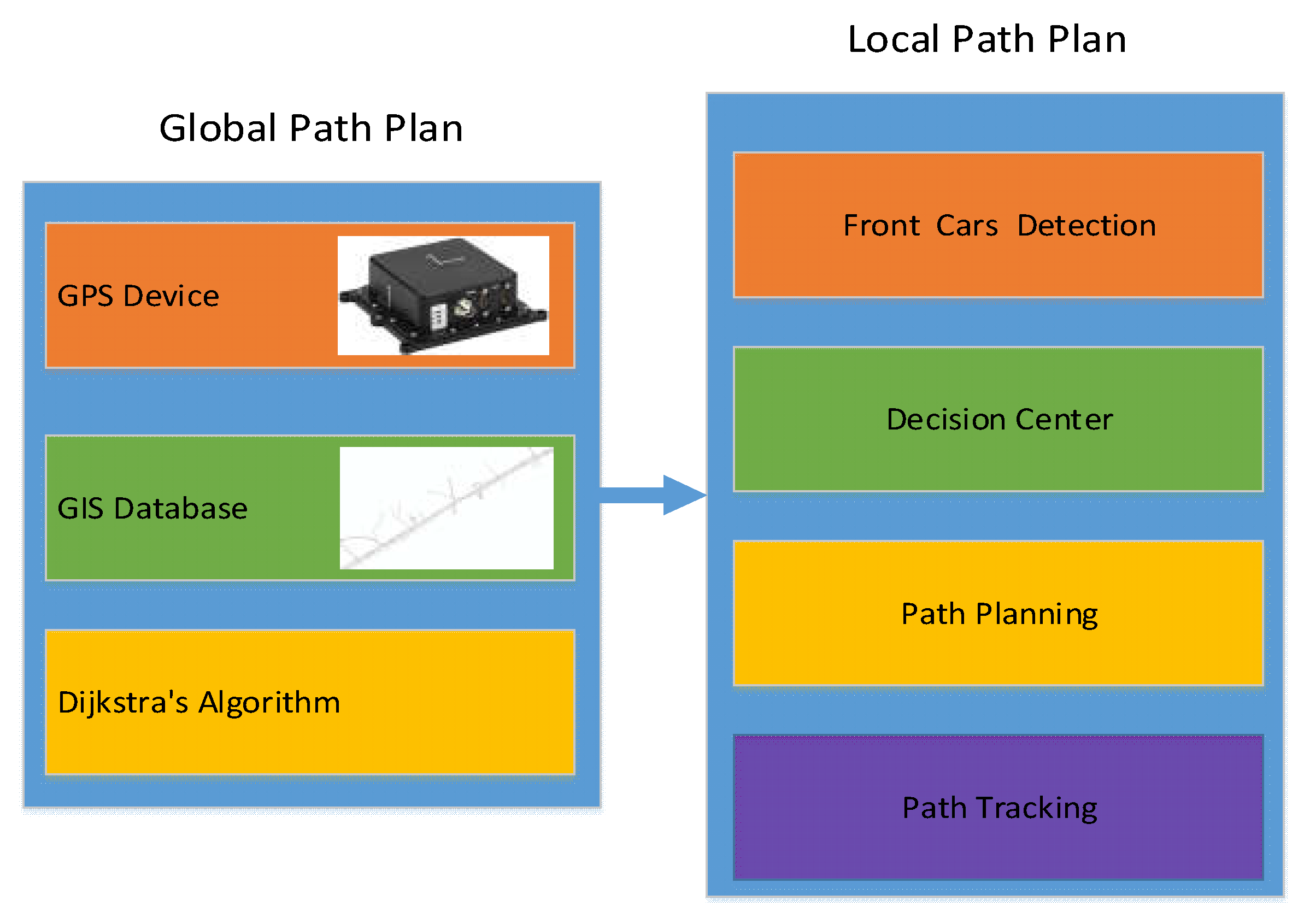
Figure 1 illustrates the path planning framework of the driverless car. By collecting environment information, the JPS (Jump Point Search)-based local path planning algorithm obtains a barrier position for avoiding obstacles. Lane tracking drives on the center of the lane. The decision center selects a reasonable driving behavior such as lane changing, overtaking, following, and so on.
3. Map Building
When a car is running on the road, it is important to select an optimal and safe driving strategy for the tracking controller, which navigates from the current position to the next destination. In other words, the controller needs some accurate GPS data to route. So, the decision center needs a high accuracy GIS map, which contains detailed and accurate GPS information about roads and special points.
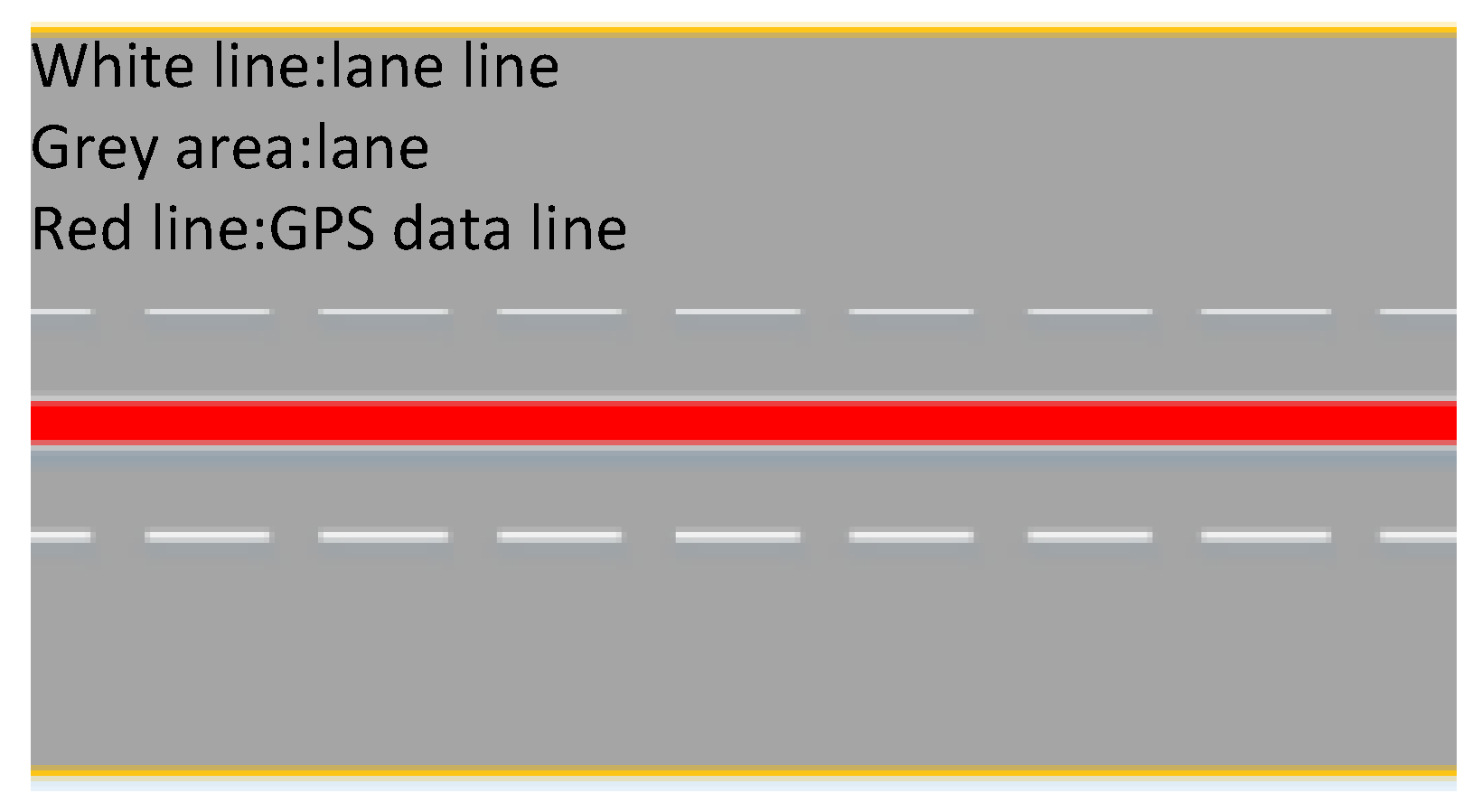
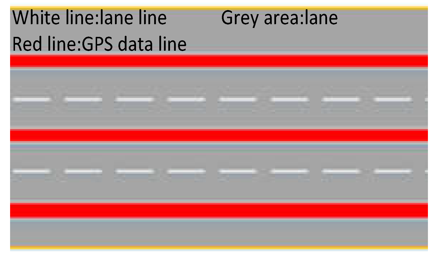
As shown in Figure 2, a road with three lanes only has a lane’s GPS data in an actual map, and the GIS system only knows the car’s lengthways position, and does not know the lateral position (as shown in Figure 3). It increases the degree of difficulty of local planning. For instance, a driverless car is driving on a road of three lanes, but it uses a general map. Or the controller intends to turn left in a crossroad, but the car is always keep in the straight lane. Thus the traffic is congested, it is difficult to change a lane currently. Whereas a high accuracy map is important for global planning, it also could lighten the load on local planning.
The mapping rules mainly contain two parts: the road (edge) and the point (junction) in Figure 4. All roads should be mapped by a straight line, and these roads are made up of a start point and an end point, and contain no break points. So, the roads’ lengths are between [5 m, 50 m]).We need to build two GPS databases, comprising a GIS database and a special route database. The GIS database stores the general road GPS data (road network information), and the special route database stores the GPS data of the route in the intersection in Figure 5.
4. Global Path Planning Based on Network Analysis Method
The global path is based on the ArcGIS Engine 10.2 [25]. We build a map layer to place the start point and the end point. Furthermore, we search a route through the road network by the Dijkstra algorithm, and build with the network analysis tool of the ArcGIS Engine-interface of INASolver.
After analysis through the tool, we get some context regarding the result. Thus the result should be the optimal path. And this result is based on length or time, which includes all feature edges and junctions. After global path planning, the feature edges and junctions information are processed.
Figure 6 depicts some insertion points in the path. These points are mapped in some special locations, such as the crossroad or the construction site. Except for some reminding information, such as the traffic signal light, all points have a unique ID number, and the unique ID number helps the global plan to seek the GPS path of this location in the special road database.
4.1. General Road Processing
When the road shows its edge feature, GPS data of the start point and the end point are gained. But, more closely, GPS points are needed for an accurate navigation. So, some insertion points between the start point and the end point are added in this edge. Due to the fact that all the edge features are mapping to the straight line, all the insertion points are on this edge. Then, we get a series of detailed GPS points for the description this path.
4.2. Special Road Processing
When the road feature is a junction in Figure 7a, and it is turning down the right path in the crossroad, so two special junction feature points are gained. If the unique number of the right point is a in Figure 7b, and the unique number of the left point is b in Figure 7a, we can get a unique index c by processing a and b in Figure 7b; then, we can search the special route database through the unique index c, so a path with some detailed GPS points is planned in Figure 7. Then, this curve path is tracked by controller according to these detailed GPS points. The radius and curvature of each of the corner points are different, so it is brief and effective to utilize the GPS points to replace the fitting curve.
4.3. The Procedure of Coordinate System Conversion
Due to the fact that the coordinate of local path planning is different from global path planning, the WGS-84 coordinate system is transferred to the local path plan coordinate, and the converting sequence is shown in Figure 8.
The GIS system is built based on the WGS-84 coordinate system [26], so the GPS coordinate data includes latitude, longitude, and elevation. The local, fixed-tangent plane is a coordinate system whose starting point is set as the origin; its x axis is the same as the orient, its y axis is the same as the north, and its z axis is the same as the vertical direction. We switch the WGS-84 coordinate system to the local fixed tangent plane through several conversions using Equation (1). Here, represents the GPS coordinate data from the GIS system, and it converts them to by Equations (1)–(2).
where is radius of curvature in prime vertical of point P, and is the first eccentricity of the ellipsoid. is a semi-major axis of the ellipsoid and a semi-minor axis of the ellipsoid.
By the same way, the coordinate of Q point is worked out by Equation (4), and P point is the origin point of the coordinate.
In the end, the point is converted to the local path coordinate by Equation (5), yaw is the car’s heading angle, and they provide for local path planning.
5. Local Path Planning Based on JPS
5.1. Jump Point Search (JPS)
JPS can quickly scan nodes from the underlying grid map to identify jump points with two simple neighbor-pruning rules. JPS is an online symmetry-breaking algorithm, which speeds up the searching path on uniform-cost grid maps by “jumping over”. Jump Point Search (JPS) is an optimization to the A* search algorithm for uniform-cost grids. It reduces symmetries in the search procedure by means of graph pruning and by eliminating certain nodes in the grid based on assumptions that can be made about the current node's neighbors, as long as certain conditions relating to the grid are satisfied. As a result, the algorithm can consider long “jumps” along straight (horizontal, vertical, and diagonal) lines in the grid, rather than the small steps from one grid position to the next that ordinary A* considers. Jump Point Search preserves A*’s optimality, while potentially reducing its running time by an order of magnitude.
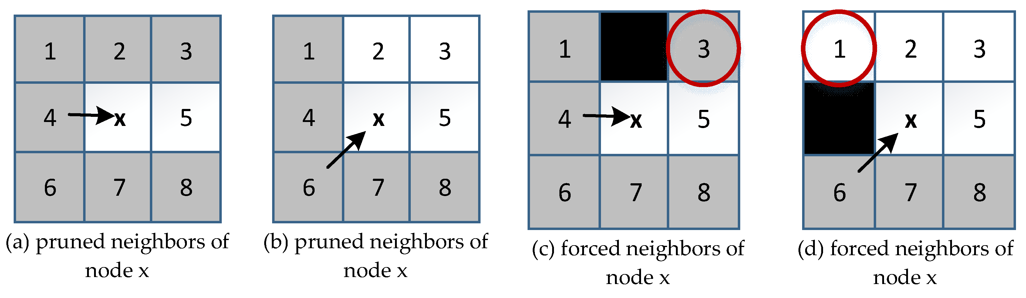
Node x is currently being expanded in Figure 9. In both cases, we can immediately prune all grey neighbors, which can reach optimally from the parent of x without ever going through node x. The arrow indicates the direction of travel from its parent, either straight or diagonal. Node x is expanded currently. The arrow indicates the direction of travel from its parent, either straight or diagonal. Note that when x is adjacent to an obstacle, the highlighted neighbors cannot be pruned in Figure 9; any alternative optimal path, from the parent of x to each of these nodes, is blocked. When you check for a node on the right of the current node of black arrow in Figure 9a,b, you should only add the node immediately to the right of the current node. For diagonal movement, we basically use the same rules as for horizontal movement, only when we move diagonal, we also check the nodes horizontally and vertically, so we are able to find a corner situation where a forced neighbor is added to the open list, or if we find our destination node in the red circle in Figure 9c,d.
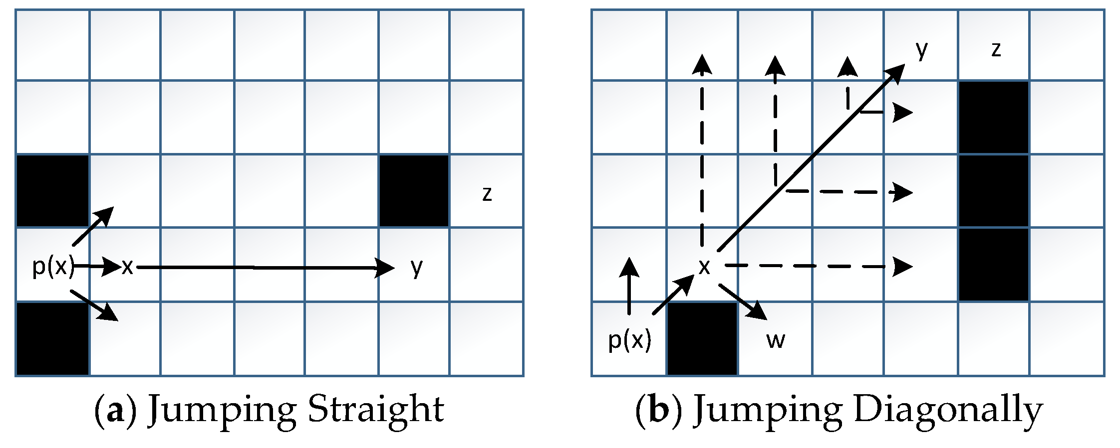
Node x is currently expanded. p(x) is its parent in Figure 10a. We recursively apply the straight pruning rule, and identify y as a jump point successor of x. Meanwhile, it has a neighbor z that cannot be reached optimally except by a path visiting x. The intermediate nodes are never explicitly generated. We recursively apply the diagonal pruning rule, and identify y as a jump point successor of x. Before each diagonal step, we cruise straight (dashed lines) first. Only if both straight recursions fail to identify a jump point do we step diagonally again. Node w is a forced neighbor of x, and it is generated as normal in Figure 10b.
5.2. Collision Car Detection
Generally, a land vehicle travels along the center of a current lane in the structured urban environment, and it prefers to go straight along the current lane. The collision car detection algorithm is divided into two parts: one is detection from the vehicle position to the control point in Figure 11, the other is detection from the control point to the adjusted return point. Here, the return point is determined by global planning. After detection, the corresponding avoiding obstacle points are planned for avoiding the collision car. Then, avoidance points are always in the center line of the left lane. Generally, the left lane is the overtaking lane in the structured urban environment.
A new trajectory is generated by Bezier curves; the current position of the vehicle, the control points, the avoidance points, and the return points are selected from the existing path. If the left lane turns to impassability, it means no avoidance point can be detected. Thus, a new trajectory is planned from the control point to a safe position in front of the collision car.
5.3. Path Generation Using JPS in Structured Urban Environment
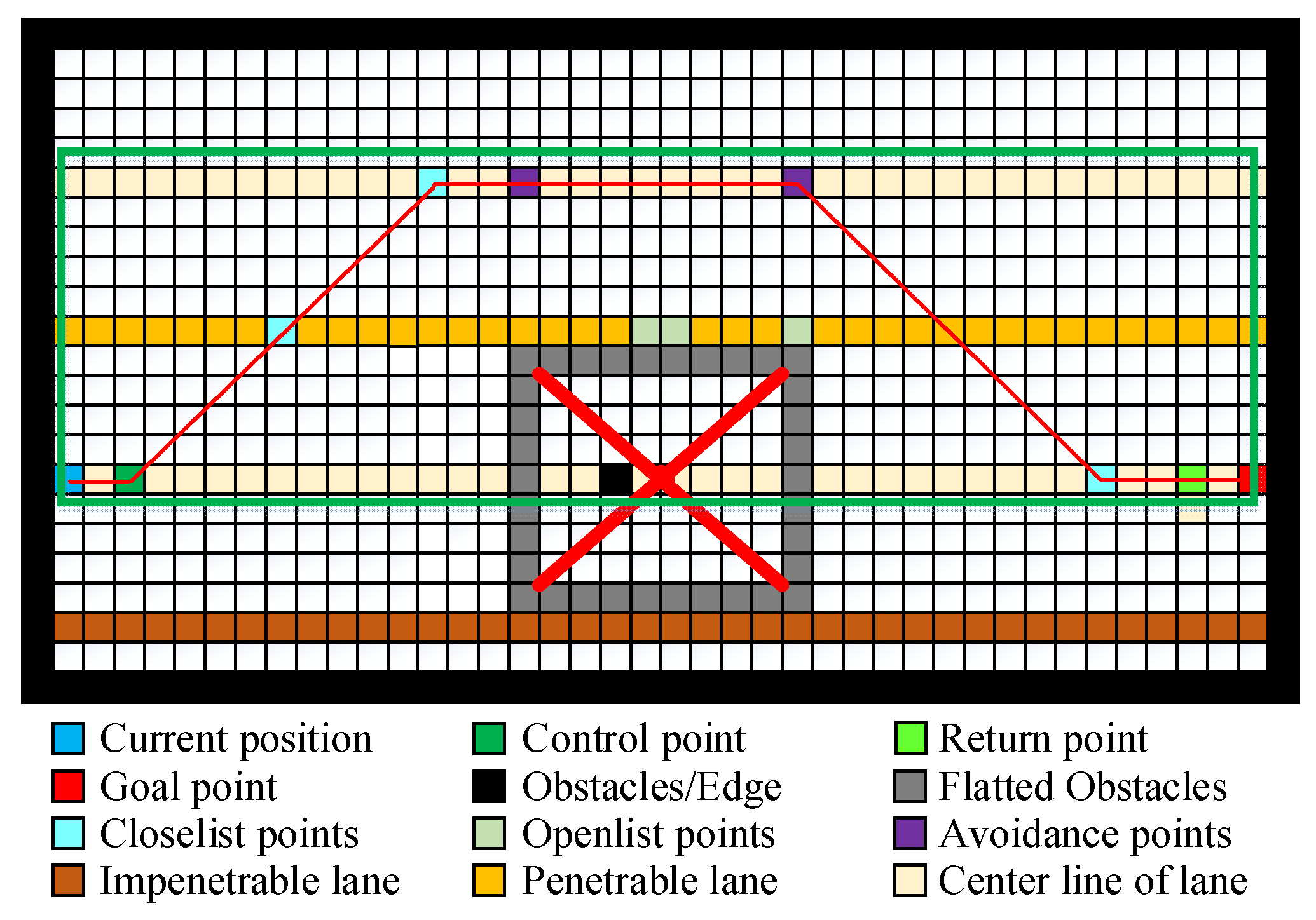
In general, cars are preferred to drive along the lane in the structured urban environment. The JPS algorithm is designed to search an optimal path from the control points to the return point, to avoid the collision in the urban environment. The JPS algorithm builds a search boundary of a green rectangle in Figure 12, and it searches Pathk from the control point to the front avoidance point according to the direction of the driving. Note that the avoidance point is closest to the flatted obstacles in the center line of the left lane; Pathk+1 is obtained by connecting the avoidance points, and Pathk+2 is searched from rear avoidance points to return points.
The path is generated from the current position to the goal point, its performances are shown in Figure 12. A vehicle is searched by JPS for a new path to avoid collision area. According to collision avoiding rule, it is indicated by a red “x” in Figure 12. The new path is determined by expanded points (open-list/close-list points); it attempts to overtake or change lane in the structured urban environment.
5.4. Trajectory Generation by Bezier Curves
A suitable spline for reducing the discrete data to a smooth path is a Bezier Curve. If those expanded points are detected successfully, they are considered as Bezier curve control points. The Bezier curve is shown in Equation (6):
where represents control points of the Bezier curves, u represents the parameters, and are known as Bernstein basis polynomials and satisfy Equations (7) and (8):
The ith path is expressed by Equation (9); it is used for generating a new path. and represent control points from the JPS algorithm, and represents Bernstein coefficients, while and represent a length of path and a limit speed of the corresponding path. Therefore, local path planning based on JPS is descripted as in Table 1.
6. Simulation Experiments Analysis
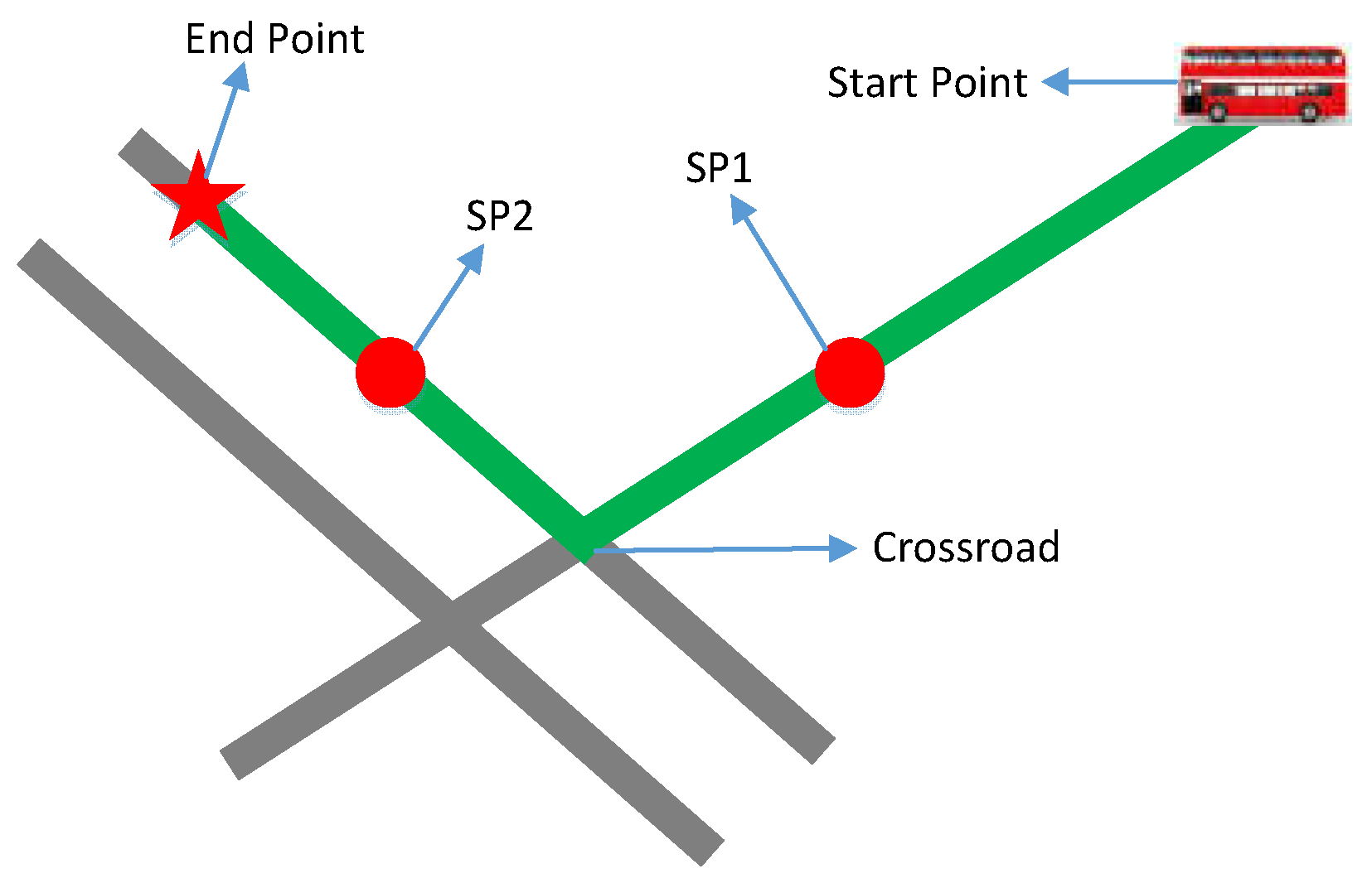
In Figure 13, an optimal route (green line) from the start point to the end point is obtained by the network analysis tool. Except for the general road, there are some special points in Figure 14.
By reading SP1 and SP2 data, the unique index is worked out, and the special route database is searched to get a special route named the Curve Path. When the car arrives at SP1, the Curve Path (red line) take the place of the green line as its current path. Also, when it arrives at SP2, it continues to use the green line as its path until it drives to the destination in Figure 14.
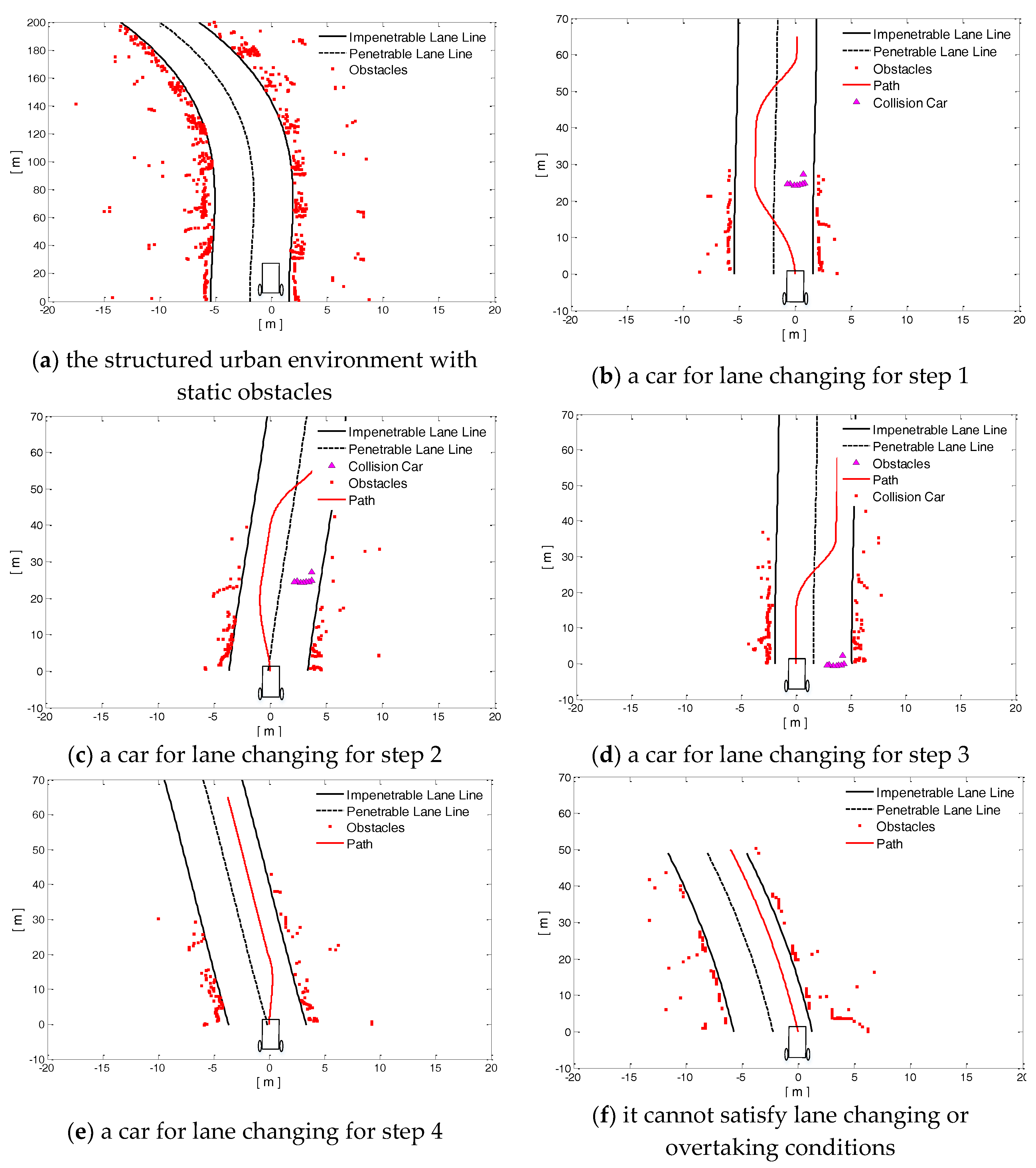
We implement the local path planning algorithm with regard to obstacles to avoid the driverless car feasible path in the structured urban environment. Firstly, static/dynamic obstacles perception and lane line detection are significant for drive behavior decisions for local path planning. In addition, the driverless car completes overtaking, unexpected obstacles avoidance, and parking. The simulation experiments results using local path planning based on JPS are as shown in Figure 15.
Figure 15a shows the experiment scene under the structured urban environment with static obstacles along the road by laser rangefinder. The black solid lines in Figure 15 represent lane lines, and the car is hard to cross, while black dash lines represents the passable lane line. The car could achieve lane changing and overtaking in Figure 15b. Figure 15c–e describes behaviors of lane changing and overtaking in the case of collision car (purple triangle) detection at the same lane. The driverless car generates a feasible trajectory to follow the local path planning as a red solid line in Figure 15. If it cannot satisfy lane changing and overtaking conditions, then the driverless car performances are shown in Figure 15f. Thus, it is verified that the proposed path planning method is effective.
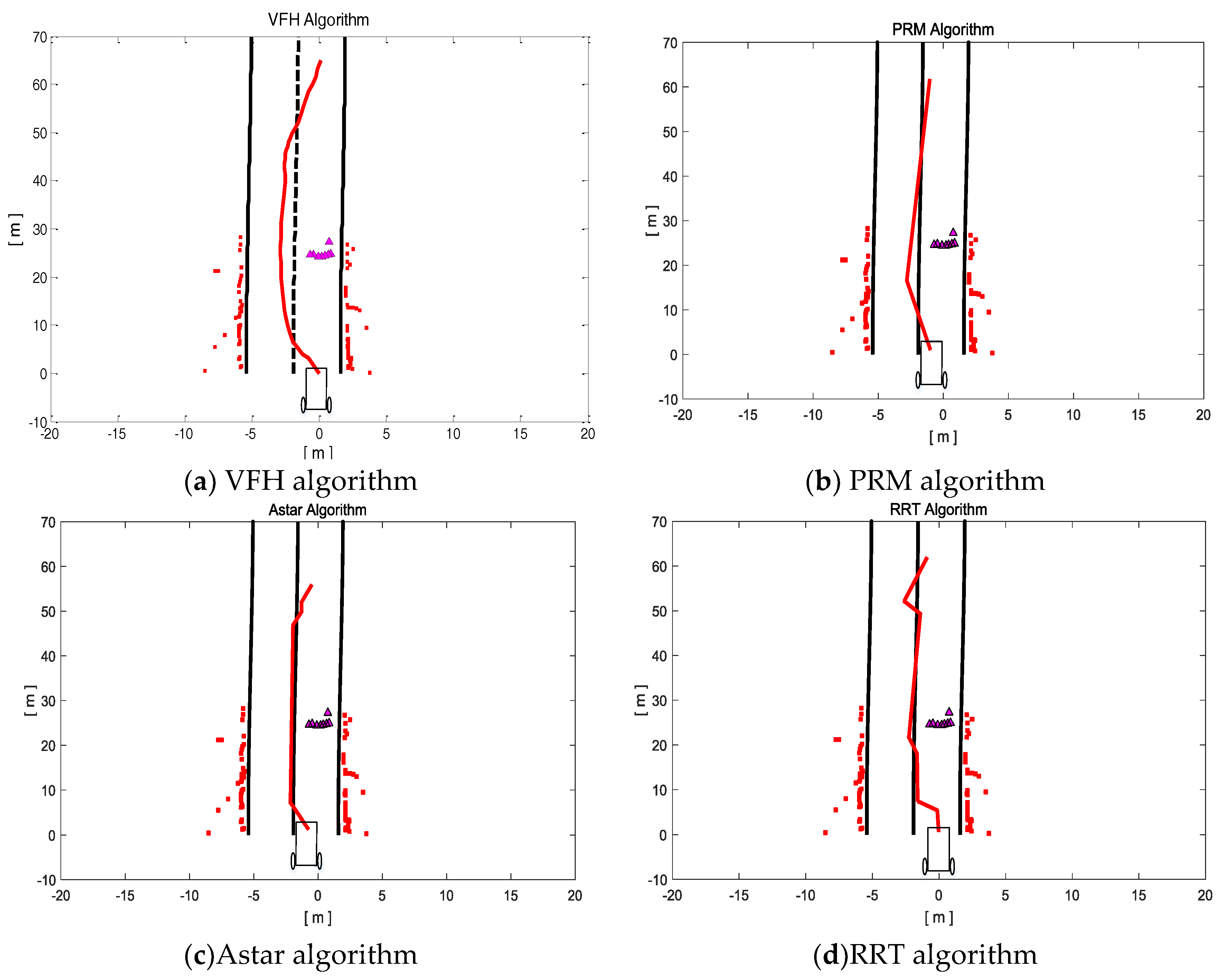
In this paper, we compare five kinds of search algorithms, including A*, JPS, PRM, VFH, and RRT. Meanwhile, experiment condition is the same as in Figure 15b. Results are shown in Table 2, and the comparison results in scene 1 are shown in Figure 16. Five different scenes of each algorithm are tested for time complexity; each scene is run five times for each algorithm in matlab to obtain an average. Therefore, the elapsed time of PRM is the longest, and the elapsed time of JPS is the shortest, which verifies that the JPS algorithm has the best performance of time cost among these popular algorithms. Meanwhile, the planning paths of A*, JPS, PRM, VFH, and RRT are different due to the different algorithm searching ability, which is another expression of time complexity.
7. Conclusions
This study presents real-time path planning based on JPS in a structured urban environment at 30 kph. At beginning, a vector GIS map is built, which contains a GPS position, a direction and lane information. Next, a global path is planned according to the GIS map database for a driverless car. Then, the JPS algorithm is adopted for driverless cars and for local path planning. Finally, 125 simulation experiment results show that the JPS algorithm is an efficient method for real-time local path planning, and it can find the optimal path rapidly in the structured urban environment.
Acknowledgments
This paper was supported by the National Natural Science Foundation of China (Grant No. 61403426, 61403427), State Key Laboratory of Mechanical Transmissions of Chongqing University (SKLMT-KFKT-201602), State Key Laboratory of Robotics and System (HIT) (SKLRS-2017-KF-13). Meanwhile, we thank Ref. [19]’s authors, Figure 9 and Figure 10 are based on that paper.
Author Contributions
Kaijun Zhou and Lingli Yu conceived and designed the experiments; Ziwei Long and Siyao Mo performed the experiments; Kaijun Zhou and Lingli Yu analyzed the data; Lingli Yu wrote the paper.
Conflicts of Interest
The authors declare no conflict of interest.
References
- Rodriguez-Castaño, A.; Heredia, G.; Ollero, A. High-speed autonomous navigation system for heavy vehicles. Appl. Soft Comput. 2016, 43, 572–582. [Google Scholar] [CrossRef]
- Shi, L.; Prevedouros, P. Autonomous and Connected Cars: HCM Estimates for Freeways with Various Market Penetration Rates. Transp. Res. Procedia 2016, 15, 389–402. [Google Scholar] [CrossRef]
- Chen, Y.; Han, J.; Wu, H. Quadratic Programming-based Approach for Autonomous Vehicle Path Planning in Space. Chin. J. Mech. Eng. 2012, 25, 665–673. [Google Scholar] [CrossRef]
- Liu, X.; Xu, X.; Dai, B. Vision-based long-distance lane perception and front vehicle location for full autonomous vehicles on highway roads. J. Cent. South Univ. 2012, 19, 1454–1465. [Google Scholar] [CrossRef]
- Kutila, M.; Pyykönen, P.; Lybeck, A.; Niemi, P.; Nordin, E. Towards Autonomous Vehicles with Advanced Sensor Solutions. World J. Eng. Technol. 2015, 3, 6–17. [Google Scholar] [CrossRef]
- Pelusi, D.; Mascella, R.; Tallini, L.; Vazquez, L.; Diaz, D. Control of Drum Boiler dynamics via an optimized fuzzy controller. Int. J. Simul. Syst. Sci. Technol. 2016, 17, 22.1–22.7. [Google Scholar]
- Sun, N.; Han, G.; Duan, P.; Tan, J. A Global and Dynamitic Route Planning Application for Smart Transportation. In Proceedings of the International Conference on Computational Intelligence Theory, Systems and Applications (CCITSA), Yilan, Taiwan, 10–12 December 2015; pp. 203–208. [Google Scholar]
- Zhu, L.; Yin, D.; Shen, L.; Xiang, X.; Bai, G. Research on urban application-oriented route planning of UAV based on mobile communication network. In Proceedings of the International Conference on Computer Science and Network Technology (ICCSNT), Harbin, China, 19–20 December 2015; pp. 1562–1570. [Google Scholar]
- Wang, J.F.; Lv, J.; Wang, C.; Zhang, Z.Q. Dynamic Route Choice Prediction Model Based on Connected Vehicle Guidance Characteristics. J. Adv. Transp. 2017. [Google Scholar] [CrossRef]
- Guo, C.; Kidono, K.; Ogawa, M. Vision-Based Identification and Application of the Leader Vehicle in Urban Environment. In Proceedings of the IEEE International Conference on Intelligent Transportation Systems, Las Palmas, Spain, 15–18 September 2015; pp. 968–974. [Google Scholar]
- Zhu, H.; Fu, M.; Yang, Y.; Wang, X.; Wang, M. A path planning algorithm based on fusing lane and obstacle map. In Proceedings of the International IEEE Conference on Intelligent Transportation Systems (ITSC), Qingdao, China, 8–11 October 2014; pp. 1442–1448. [Google Scholar]
- Ma, Y.J.; Hou, W. Path planning method based on hierarchical hybrid algorithm. In Proceedings of the International Conference on Computer, Mechatronics, Control and Electronic Engineering, Changchun, China, 24–26 August 2010; pp. 74–77. [Google Scholar]
- Lidoris, G.; Rohrmuller, F.; Wollherr, D.; Buss, M. The Autonomous City Explorer (ACE) project—Mobile robot navigation in highly populated urban environments. In Proceedings of the IEEE International Conference on Robotics and Automation, Kobe, Japan, 12–17 May 2009; pp. 1416–1422. [Google Scholar]
- Ulrich, I.; Borenstein, J. VFH*: Local obstacle avoidance with look-ahead verification. In Proceedings of the IEEE International Conference on Robotics and Automation, San Francisco, CA, USA, 24–28 April 2000; Volume 3, pp. 2505–2511. [Google Scholar]
- Sun, F.; Huang, Y.; Yuan, J.; Kang, Y.; Ma, F. A Compound PRM Method for Path Planning of the Tractor-Trailer Mobile Robot. In Proceedings of the IEEE International Conference on Automation and Logistics, Jinan, China, 18–21 August 2007; pp. 1880–1885. [Google Scholar]
- Tian, Y.; Yan, L.; Park, G.Y.; Yang, S.H.; Kim, Y.S.; Lee, S.R.; Lee, C.Y. Application of RRT-based local Path Planning Algorithm in Unknown Environment. In Proceedings of the International Symposium on Computational Intelligence in Robotics and Automation, Jacksonville, FL, USA, 20–23 June 2007; pp. 456–460. [Google Scholar]
- Majumder, S.; Prasad, M.S. Three dimensional D* algorithm for incremental path planning in uncooperative environment. In Proceedings of the International Conference on Signal Processing and Integrated Networks (SPIN), Noida, India, 11–12 February 2016; pp. 431–435. [Google Scholar]
- Jiang, W.L.; Rong, X.; Jian, C. Sideslip-force based local path planning in complex and dynamic environment. J. Zhejiang Univ. 2007, 41, 1609–1614. [Google Scholar]
- Harabor, D.D.; Grastien, A. Online Graph Pruning for Pathfinding on Grid Maps. In Proceedings of the AAAI Conference on Artificial Intelligence, San Francisco, CA, USA, 7–11 August 2011; pp. 1114–1119. [Google Scholar]
- Harabor, D.; Grastien, A. Improving jump point search. In Proceedings of the Twenty-Fourth International Conference on Automated Planning and Scheduling, Portsmouth, NH, USA, 21–26 June 2014; pp. 128–135. [Google Scholar]
- Rabin, S.; Sturtevant, N.R. Combining Bounding Boxes and JPS to Prune Grid Pathfinding. In Proceedings of the AAAI Conference on Artificial Intelligence, Phoenix, AZ, USA, 12–17 February 2016; pp. 746–752. [Google Scholar]
- Aversa, D.; Sardina, S.; Vassos, S. Path planning with Inventory-driven Jump-Point-Search. In Proceedings of the AAAI Conference on Artificial Intelligence and Interactive Digital Entertainment (AIIDE), Santa Cruz, CA, USA, 14–18 November 2015; pp. 2–8. [Google Scholar]
- Jiang, K.; Yang, Y. Efficient dynamic pruning on largest scores first (LSF) retrieval. Front. Inf. Technol. Electron. Eng. 2016, 17, 1–14. [Google Scholar] [CrossRef]
- Khan, H.; Iqbal, J.; Baizid, K.; Zielinska, T. Longitudinal and lateral slip control of autonomous wheeled mobile robot for trajectory tracking. Front. Inf. Technol. Electron. Eng. 2015, 16, 166–172. [Google Scholar]
- Available online: http://www.esri.com/software/arcgis/arcgisengine (accessed on 23 August 2017).
- Available online: http://gisgeography.com/wgs84-world-geodetic-system/ (accessed on 23 August 2017).
Figure 1.
Path planning framework of driverless car.

Figure 2.
The general map has only one Global Positioning System (GPS) data line.

Figure 3.
Every lane has its own GPS data line in the high accuracy Geographic Information System (GIS).
Figure 3.
Every lane has its own GPS data line in the high accuracy Geographic Information System (GIS).

Figure 4.
A road (edge) feature only has one start point and one end point, but no break point.

Figure 5.
The special points (junction) are placed nearby in the crossroad.
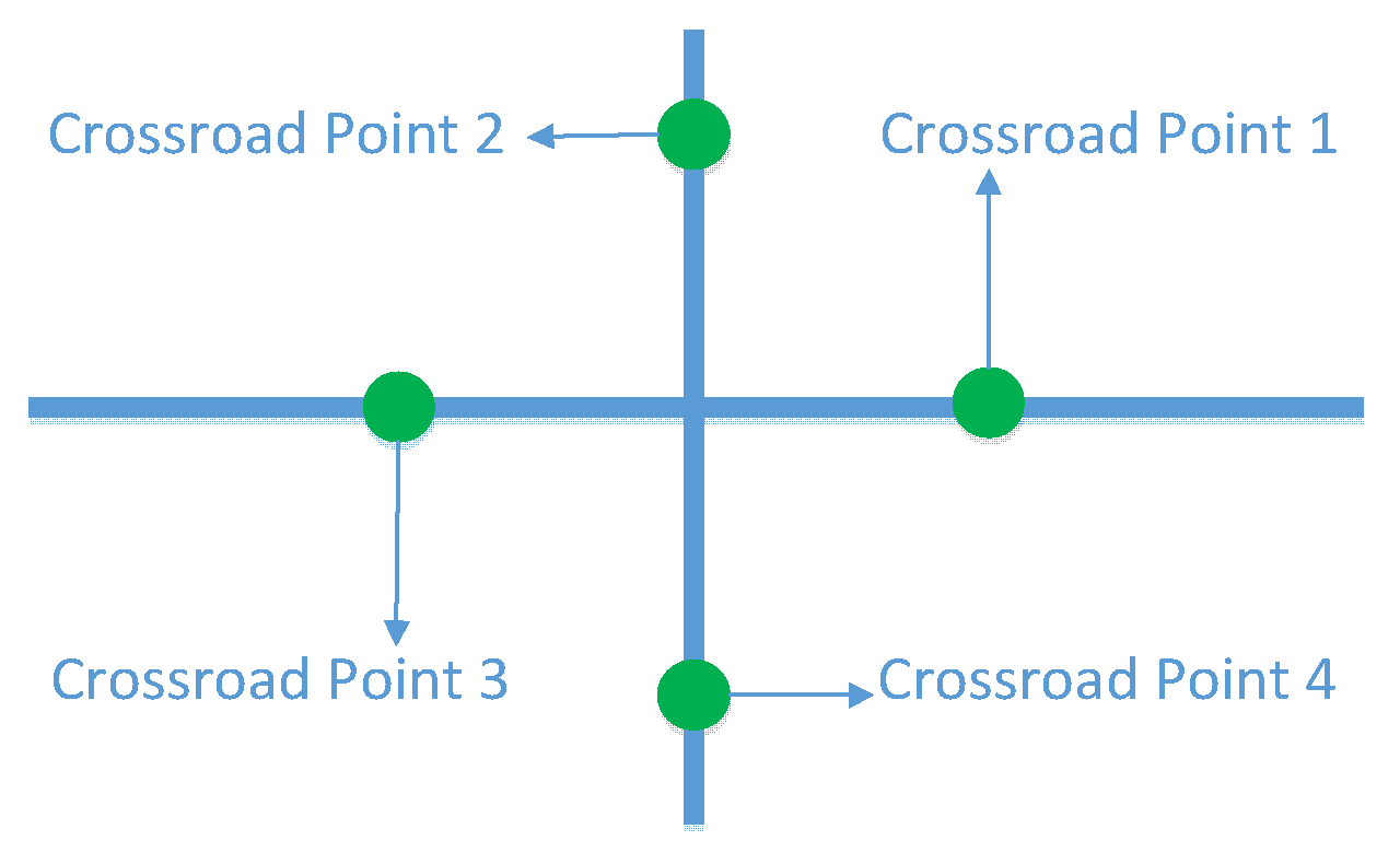
Figure 6.
Some insertion points are placed in the path.
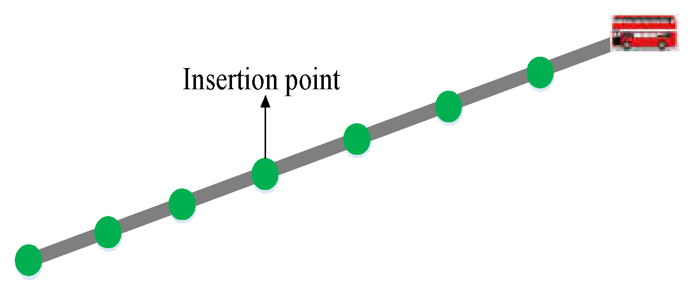
Figure 7.
Two special points and GPS points with the unique index in the crossroad.
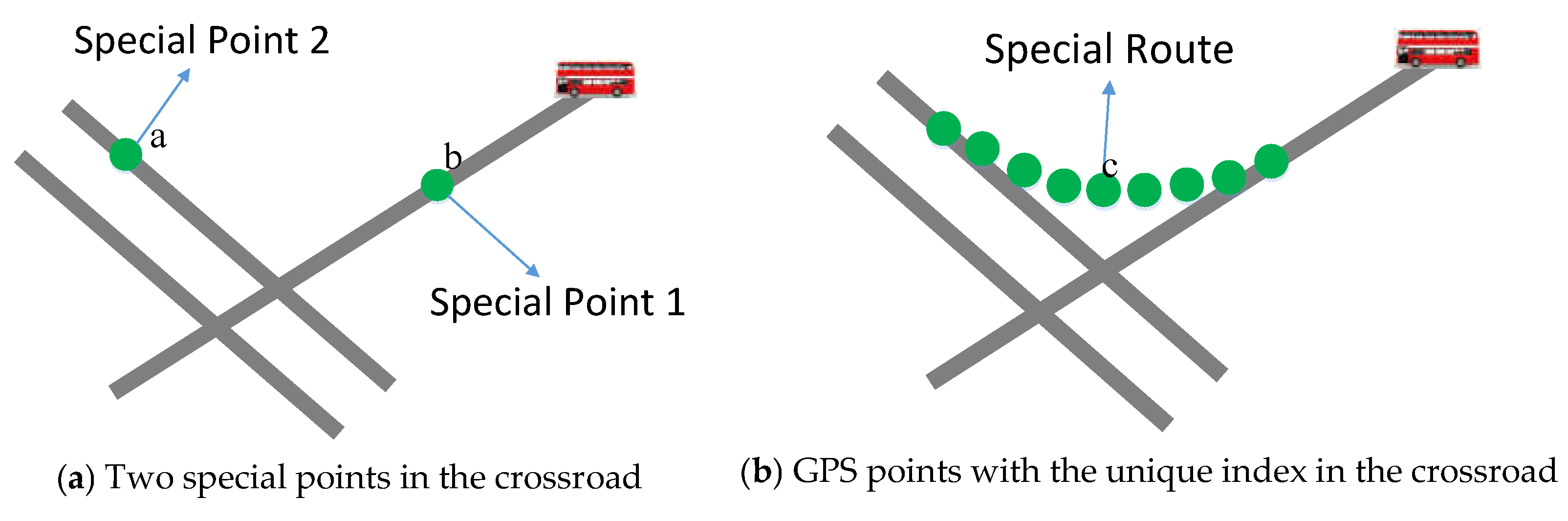
Figure 8.
The converting sequence of several coordinate systems.
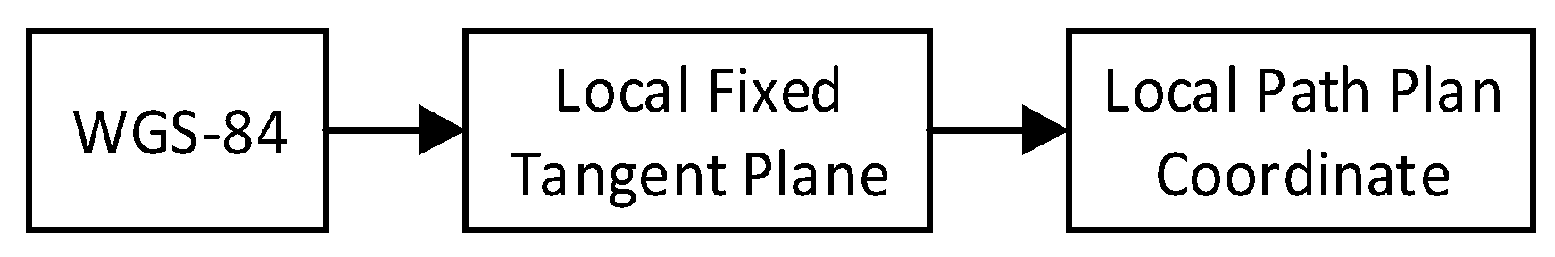
Figure 9.
Neighbor Pruning and Forced Neighbor.

Figure 10.
Successful straight and diagonal jumps with the JPS algorithm by applying pruning and forced neighbor rules.
Figure 10.
Successful straight and diagonal jumps with the JPS algorithm by applying pruning and forced neighbor rules.

Figure 11.
Detection of collision car and avoidance points.
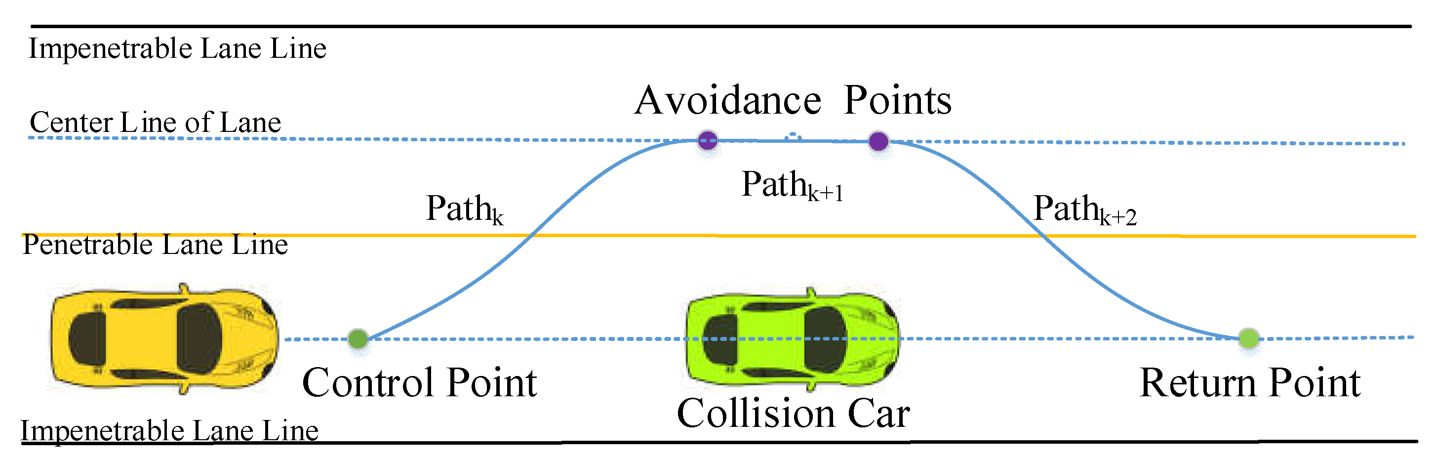
Figure 12.
Jump Point Search (JPS) search procedure.

Figure 13.
The results of global path planning.

Figure 14.
Search and get the special Curve Path.
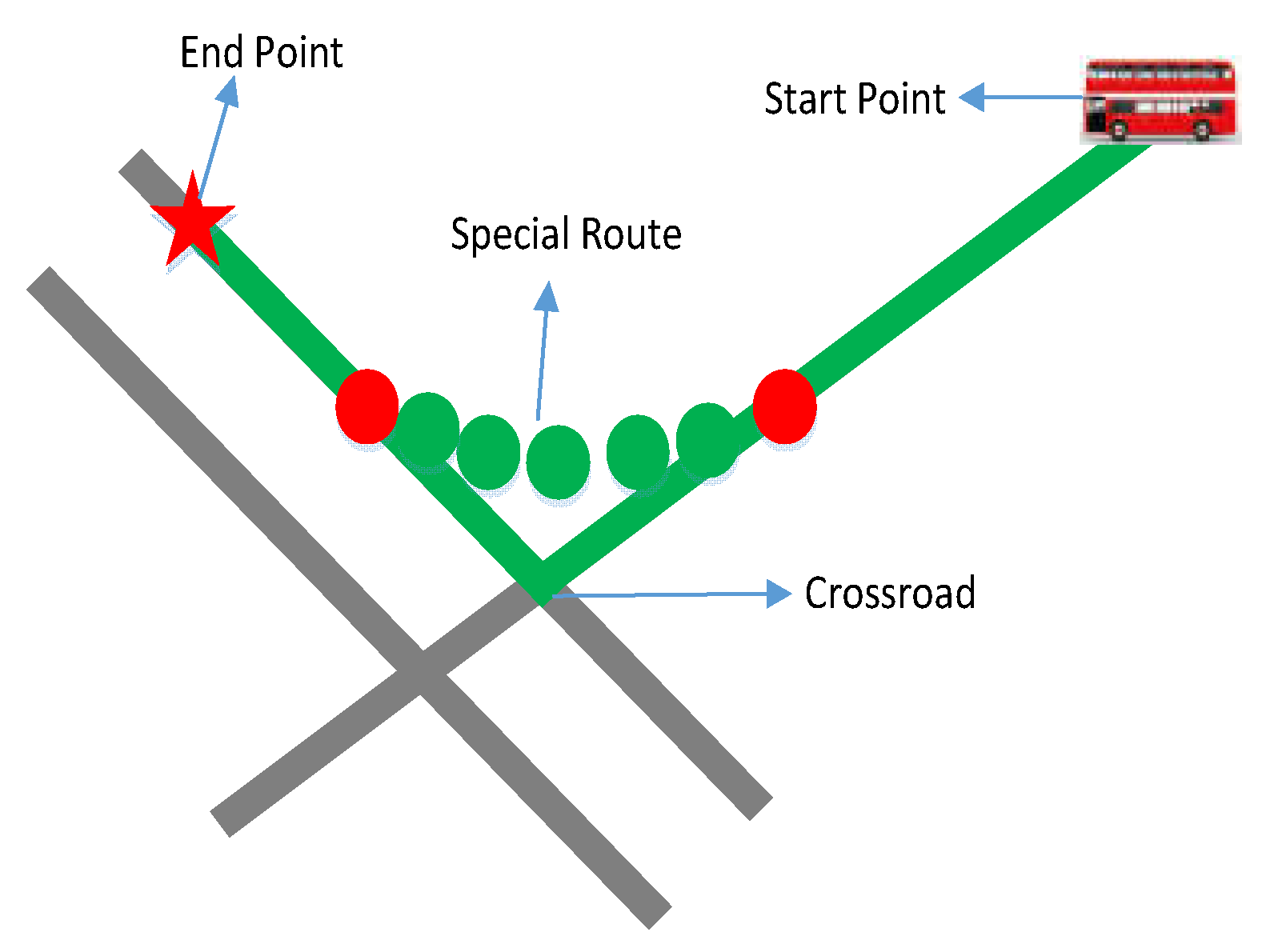
Figure 15.
Path planning results for driverless car in structured urban environment.

Figure 16.
Four algorithms simulation experiment results.

Table 1.
Local Path Planning based on JPS in Structured Environment.
| Step1: Drive behavior decisions, meanwhile, detection of collision car includes two parts, one is detection from vehicle position to control point, the other is detection from control point to adjusted return point; |
| Step2: Structure of searching boundary and avoidance points in the structured urban environment; |
| Step3: Path generation with JPS in Section 4.3; |
| Step4: Trajectory smoothing with Bezier curves in Section 5.4. |
Table 2.
The time complexity evaluation comparison (secs) of different algorithms.
| Algorithm | Scene1 | Scene2 | Scene3 | Scene4 | Scene5 | Average |
|---|---|---|---|---|---|---|
| A* | 0.5226 | 0.4689 | 0.4241 | 0.4327 | 0.6288 | 0.8257 |
| JPS | 0.02113 | 0.01792 | 0.02003 | 0.0179 | 0.0259 | 0.02058 |
| PRM | 8.2568 | 6.2625 | 6.7503 | 7.0778 | 6.9995 | 7.0694 |
| VFH | 1.3215 | 1.0611 | 1.2958 | 1.0376 | 1.1192 | 1.1670 |
| RRT | 0.0900 | 0.1085 | 0.0703 | 0.0777 | 0.0834 | 0.0860 |
© 2017 by the authors. Licensee MDPI, Basel, Switzerland. This article is an open access article distributed under the terms and conditions of the Creative Commons Attribution (CC BY) license (http://creativecommons.org/licenses/by/4.0/).
Share and Cite
MDPI and ACS Style
Zhou, K.; Yu, L.; Long, Z.; Mo, S. Local Path Planning of Driverless Car Navigation Based on Jump Point Search Method Under Urban Environment. Future Internet 2017, 9, 51. https://doi.org/10.3390/fi9030051
AMA Style
Zhou K, Yu L, Long Z, Mo S. Local Path Planning of Driverless Car Navigation Based on Jump Point Search Method Under Urban Environment. Future Internet. 2017; 9(3):51. https://doi.org/10.3390/fi9030051
Chicago/Turabian StyleZhou, Kaijun, Lingli Yu, Ziwei Long, and Siyao Mo. 2017. "Local Path Planning of Driverless Car Navigation Based on Jump Point Search Method Under Urban Environment" Future Internet 9, no. 3: 51. https://doi.org/10.3390/fi9030051
Note that from the first issue of 2016, this journal uses article numbers instead of page numbers. See further details here.