Article

Density Self-Adaptive Hybrid Clustering Routing Protocol for Wireless Sensor Networks

1
School of Computer and Software, Nanjing University of Information Science & Technology, Nanjing 210044, Jiangsu, China
2
Jiangsu Collaborative Innovation Center on Atmospheric Environment and Equipment Technology, Nanjing 210044, Jiangsu, China
3
Jiangsu Engineering Center of Network Monitoring, Nanjing University of Information Science and Technology, Nanjing 210044, Jiangsu, China
*
Authors to whom correspondence should be addressed.
Future Internet 2016, 8(3), 27; https://doi.org/10.3390/fi8030027
Submission received: 18 April 2016 / Revised: 21 June 2016 / Accepted: 22 June 2016 / Published: 29 June 2016

Abstract

:
Energy efficiency is of major concern in wireless sensor networks, especially in difficult node deployment environments. Clustering is an effective method to save energy consumption and prolong the network lifetime. There are two kinds of clustering methods in hierarchical routing protocols, namely distributed control and centralized control. In the distributed strategy, the algorithm has good scalability, but it can easily lead to an uneven distribution of cluster heads. When the centralized strategy is used, the network is balanced and robust, but the overhead of clustering is large and the network latency is increased. In our proposed protocol, named DAHC, a mixture algorithm of distributed and centralized control is used to select a cluster head (CH). Simultaneously, we propose a novel approach to judge the cluster density and adjust according to the preset threshold. The simulation results show that our methods can evenly distribute the energy load on all nodes, save the energy consumption of communication and extend the network lifetime concurrently.

1. Introduction

Wireless sensor networks (WSNs) are composed of a large number of low-cost micro sensor nodes with processing, storing, and communicating capabilities [1]. With the development of technology, WSNs have been applied to many fields, such as environmental monitoring [2,3], object tracking [4], healthcare system [5], and some others.
In wireless sensor networks, the main task of the routing protocol is to establish the route from source node to sink node, and transmit data reliably. In routing protocols, the efficiency of energy, the reliability of data transmission [6], authentication [7], and the low latency of the network construction [8], are all research hotspots. Among them, the problem of energy consumption is of major concern. Clustering is a basic method to design the energy efficient, robust, and scalable sensor networks [9]. It uses the rotation of cluster heads (CHs) to balance the energy consumption to all nodes, so as to improve the energy efficiency. In terms of the CH generation mode, there are distributed and centralized strategies. In the distributed way, there is no control center in the network, and the node itself decides whether to become a CH or not. This algorithm has good scalability, but it can easily lead to uneven distribution of CHs, so the load balance of the cluster is poor. When the centralized strategy is adopted, all of the nodes transmit the energy and location information to the base station (BS). Then, the BS selects the suitable CHs. As the selection is based on global information, the distribution of CHs is more reasonable and the energy load is relatively balanced. However, the communication with the BS each round wastes a lot of energy and increases the network delay.
Thus, our work is to study the problem of clustering in hierarchical routing protocols. In order to evenly distribute the energy to each node and prolong the network lifetime, we propose a new algorithm to select the CHs. In our proposed algorithm, the distributed and centralized methods are used in a mixed way to select CHs. In this way, it combines the advantages of both in order to save energy and ensure the rationality of CH distribution. In addition, we propose a scheme for the cluster density adjusting to achieve a balanced energy load.
The remainder of this paper is organized as follows: Section 2 briefly reviews some clustering protocols. The DAHC protocol is described in Section 3. Section 4 evaluates the performance through simulation results, and finally Section 5 will draw our conclusions.

2. Related Work

The LEACH protocol proposed by Heinzelman et al. [
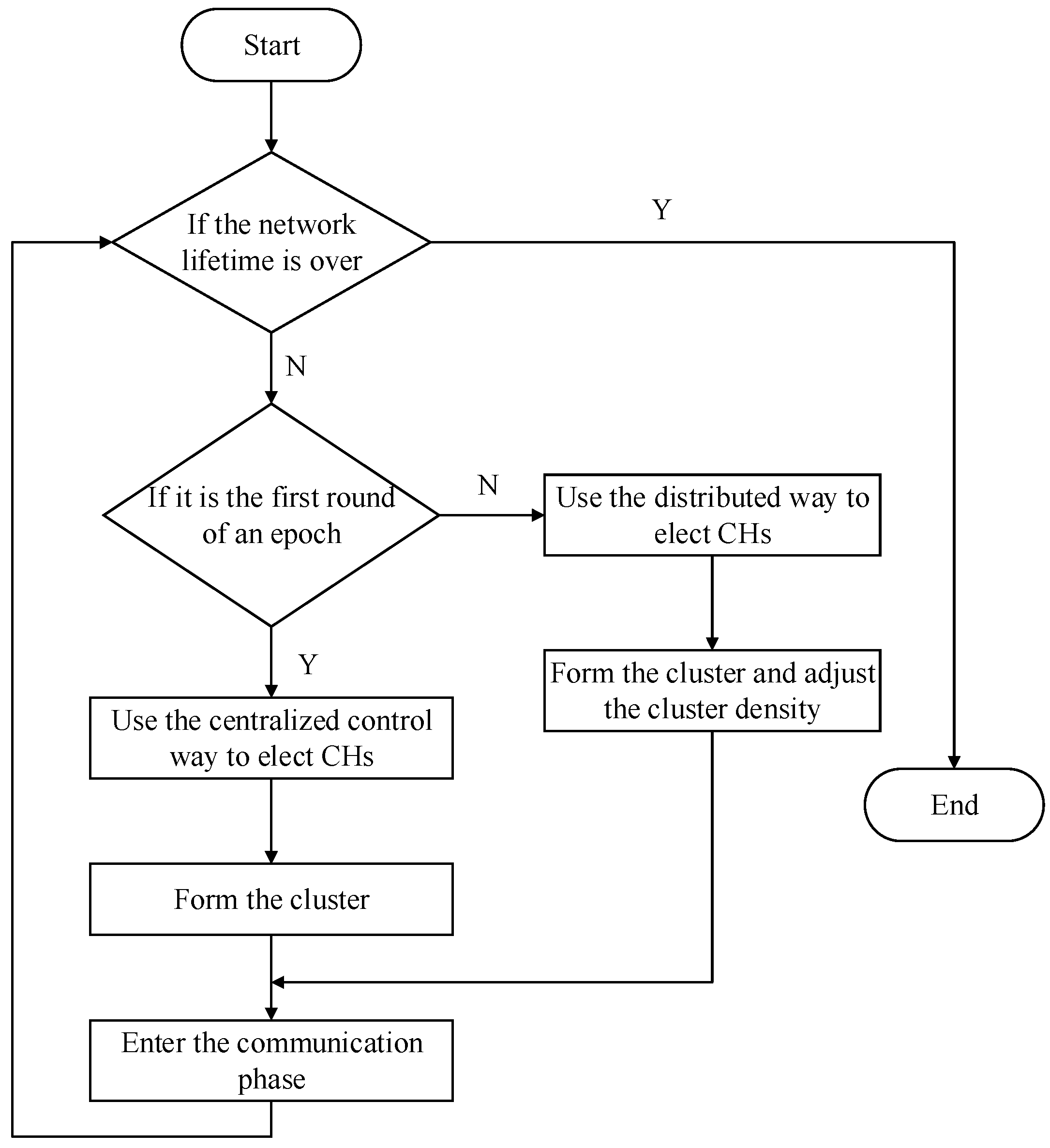
10] is the earliest clustering protocol, which has very important influence on the later clustering routing protocols. In the LEACH protocol, the implementation of the algorithm is performed circularly. Each round is made up of two stages. One is the establishment of the cluster, and the other is the stable data communication phase. In the establishment stage, each node generates a random number between 0 and 1, then the random number is compared with the preset threshold T(n). If the random number is less than T(n), the node will be selected as a cluster head (CH). The selection of CHs each round is produced from the nodes that have not been selected as a CH, so, the threshold value of the nodes that have been selected as a CH is 0. The threshold is set as:
T ( n ) = { P 1 P × [ r mod ( 1 / P ) ] , n G 0 , else
where P is the percentage of cluster heads in all nodes, r is the current round number, n is the token of node, and 
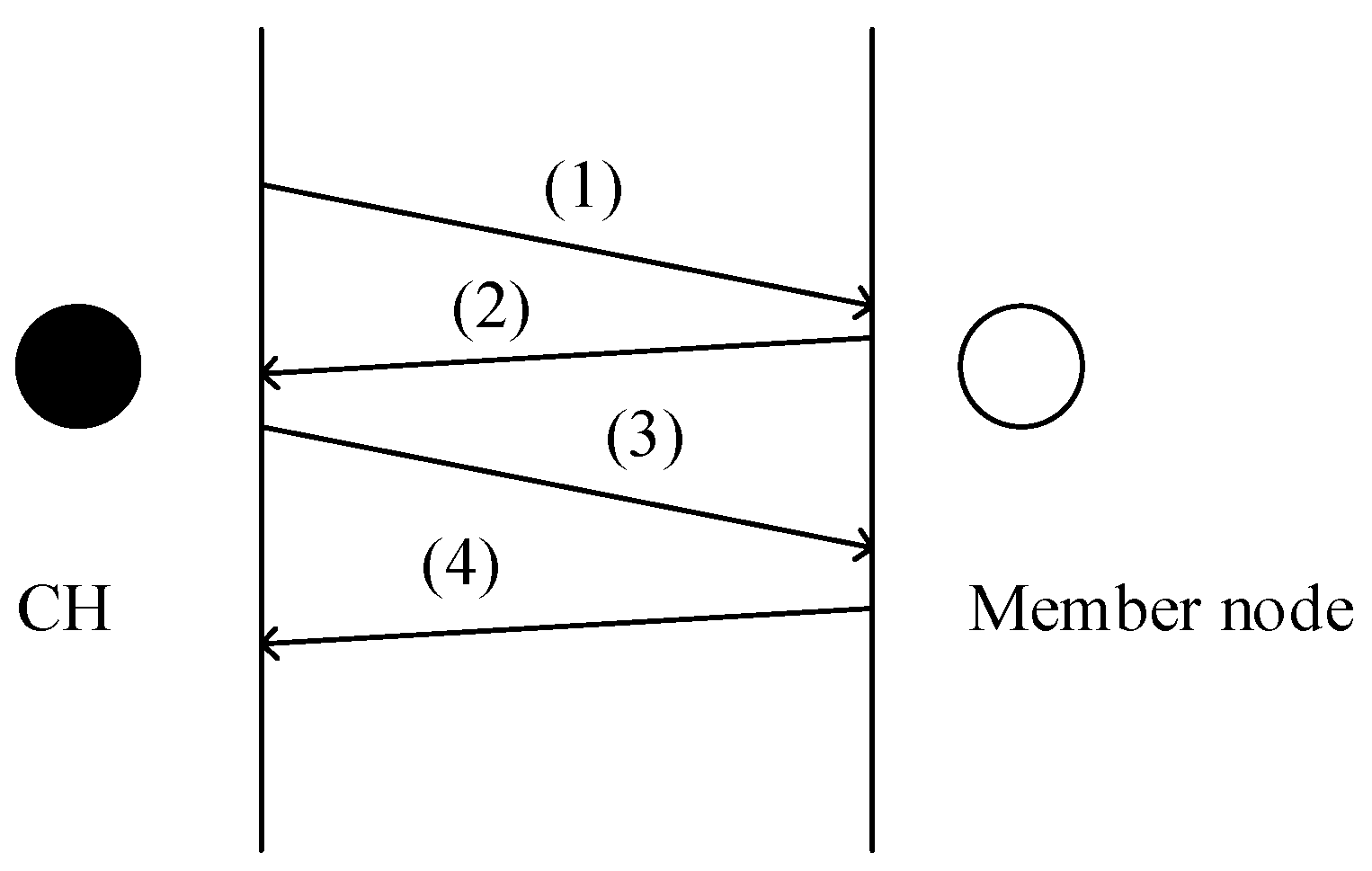
G represents the set of all nodes that have not been selected as a CH. Then, the nodes will choose the proper CH as its manager. After the cluster structure is formed, the data communication phase is entered. In this stage, CHs will assign a TDMA (Time Division Multiple Access) schedule and inform all nodes. The nodes transmit data to the CH during the corresponding time slot, and the CHs transmit the results to the BS after the fusion processing. Compared with the flat routing, although the LEACH protocol has balanced the energy load of the whole network, it does not consider the residual energy of the node, and it selects CHs in a random way, resulting in uneven distribution of the CHs.
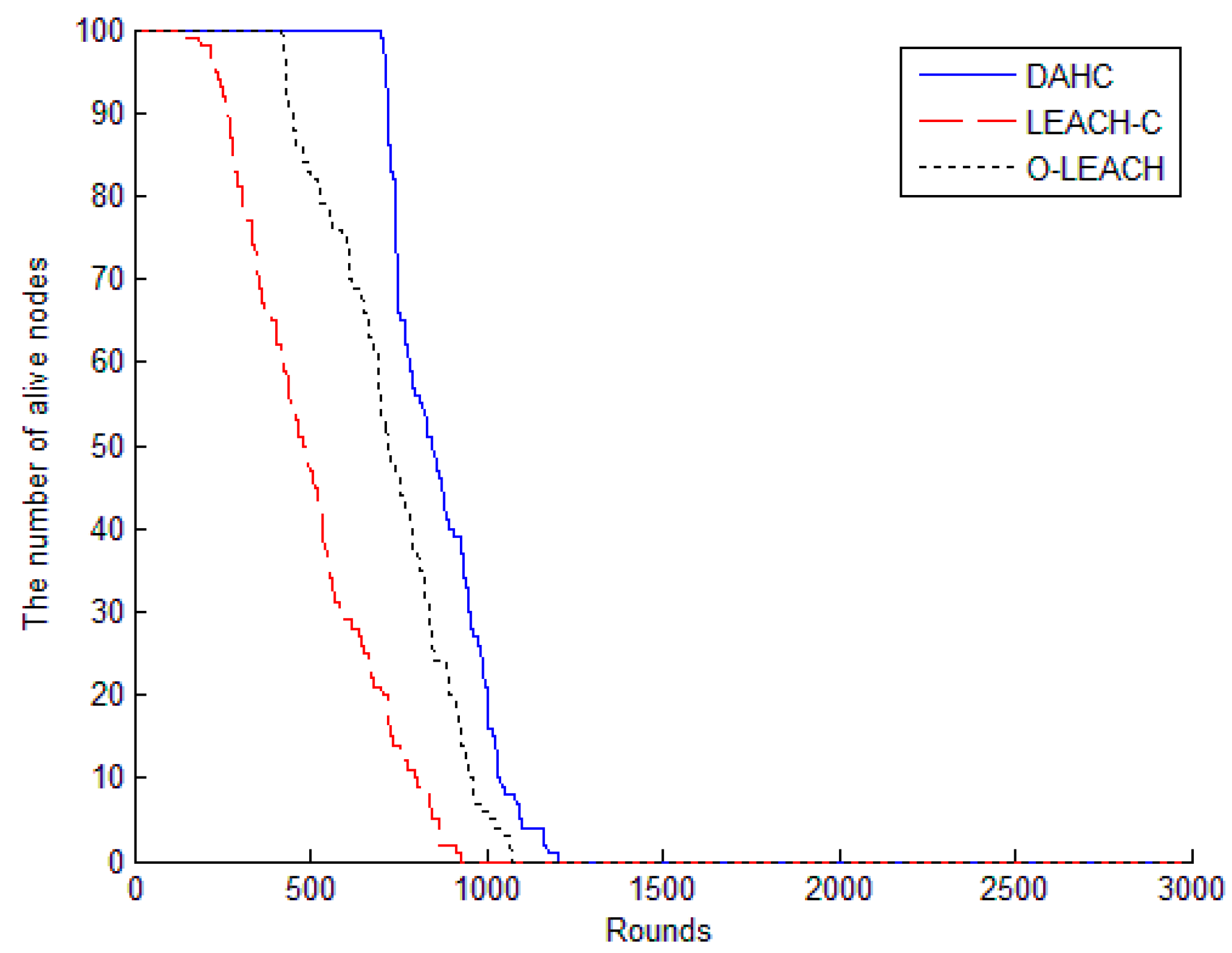
The LEACH-C protocol [
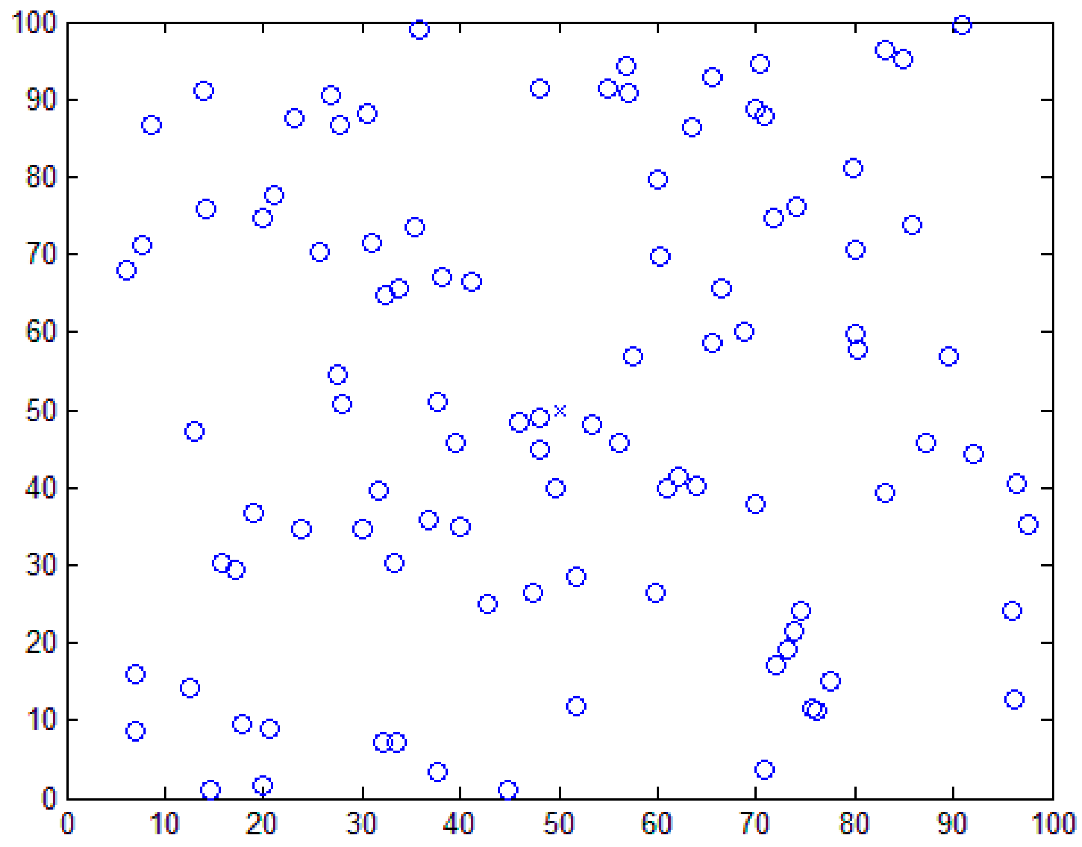
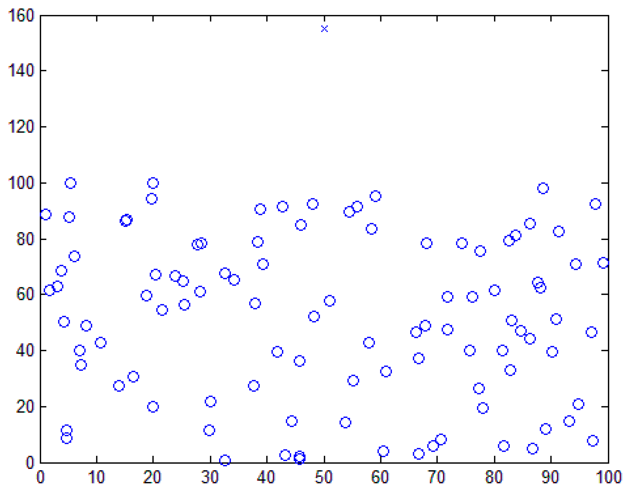
11] is modified on the basis of LEACH. Its cluster head selection method adopts centralized control rather than a distributed method. It selects CHs in the sink node based on the global information of all nodes. Each node reports its geographic position and the current energy to the BS. Then, the BS will calculate the average energy. The node whose current energy is higher than the average energy will be the candidate cluster head. After that, a simulated annealing algorithm is used to select the appropriate number and optimal location of the cluster heads from the candidate nodes. Finally, the BS will broadcast the set of cluster heads, and the rest of the operation is the same as LEACH. This method solves the problem of uneven distribution of cluster heads that LEACH has, but the nodes need to communicate with the base station each round, leading to extra energy consumption. O-LEACH [12] is another extension of LEACH, in which the nodes with more energy are more likely to be a CH. It takes the remaining energy into account. As a result, it lengthens the network lifetime to some extent.
Younis describes the implementation of the HEED protocol in [13]. It mainly considers the primary and secondary parameters. The primary parameter is the residual energy of the node, and the secondary parameter is the transmission energy consumption within the cluster. It improves the energy efficiency and further prolongs the life cycle of the network. However, there still exists a shortcoming that cannot be overcome, namely, the problem of false cluster heads. Recently, a lot of clustering protocols have been improved. Shokouhifar proposes the ASLPR protocol in [14], which takes four factors into account: the residual energy of nodes, the distance from node to the base station, the number of CHs in the current round, and the total number of nodes that have been selected as a cluster head so far. In addition, the SEECH protocol [15] selects the cluster heads and relay nodes separately to save the energy of CHs.

3. The Design of DAHC Protocol

This paper aims to study how to reduce the energy consumption of the nodes, balance the energy load of the cluster, and prolong the network lifetime. In previous clustering research work, researchers usually choose distributed or centralized control to select the CHs. These two methods have advantages and disadvantages. In view of previous discussions, we put forward the DAHC protocol. In this protocol, the distributed and centralized control methods are used to select the CHs in a mixed way. Simultaneously, in order to solve the problem of uneven distribution of CHs caused by the distributed method, a novel way of adaptive cluster density is proposed. The implementation process of the DAHC protocol is described in detail as follows.

3.1. Communication Model

In this paper, the calculation of energy consumption uses the same radio model as stated in [11]. In this model, to transmit an l-bit message from transmitter node to receiver node over a distance d, the respective consumption is:
E T x ( l , d ) = E T x _ e l e c ( l ) + E T x _ a m p ( l , d ) = { l × E e l e c + l × ε f s × d 2 , d < d 0 l × E e l e c + l × ε m p × d 4 , d d 0
E R x ( l ) = E R x _ e l e c ( l ) = l × E e l e c
where d 0 is set as d 0 = ε f s / ε m p , E e l e c (per bit) is the energy dissipation to run either the transmitter or the receiver circuitry, and it depends on factors, such as the digital coding, modulation, filtering, and spreading of the signal. Additionally, ε f s and ε m p are the amplification coefficients of the power-amplifier in the free space and the multipath fading channel models, respectively. With the communication model, the node calculates the energy consumption based on the length of information and the distance between transmitter and receiver. If the distance is less than d 0 , the overhead is calculated according to Equation (2), otherwise it is computed according to Equation (3).

3.2. Overall Operation of DAHC Protocol

Similar to other clustering protocols, the operation of DAHC in each round can be separated into the setup phase and the communication phase. During the setup phase, CHs are chosen by the relevant method. First of all, we introduce the concept of epoch. In the WSNs, if the proportion of the CHs in all nodes is P, then 1/P is an epoch. When the CH is selected by the centralized control method, the CH will do the corresponding calculation work and make preparations for the next election. In a centralized strategy, the energy consumption includes the communication between nodes and the BS and the cost of member nodes joining the cluster each round. When using a distributed method, the nodes will generate CHs according to the calculated information of the first round of the epoch, judge the cluster density in the final stage of clustering, and make the corresponding adjusting operation. In this method, the energy consumption contains the communication between nodes and the BS at the first round of the epoch, and the cost of member nodes joining to cluster each round. In the rest of the rounds of an epoch, the forming cluster dissipates more energy because it has twice as many interactions with the CH than the centralized method. However, the cost of more interactions is much less than the communication with the BS due to the shorter distance. After the formation of the cluster, it enters a stable data communication phase. In this phase, each CH will allocate a TDMA schedule. Thus, the member nodes send data to the CH during the corresponding time slot and stay asleep at other times. After the aggregation of received data packets, the CHs will send the results to the BS. After a given time spent on the communication, the network goes into the next cycle until the end of the network lifetime. The flow chart of the DAHC protocol is shown in Figure 1:

3.3. The Election of CHs

The DAHC protocol uses a hybrid method to select CHs. In clustering protocols, the algorithm is cycled based on the round, and the operation of each round is the same. In our proposed protocol, the execution of the algorithm is also cycled by epoch. In the first round of an epoch, CHs are produced by the BS through centralized control. This is the same as the LEACH-C protocol, where each node sends its own energy information and geographic location to the BS, and the BS uses the simulated annealing algorithm to select the appropriate number and the optimal location of the nodes as the CHs. Only the first round of each epoch is generated by a centralized control method. After the selection, the BS will broadcast the CH set and the cluster structure, and the nodes will be assigned with roles according to the received information. After this step, the clustering process is completed.
In the rest of the rounds of an epoch, aiming to save the communication cost between nodes and the BS, cluster heads are selected by a distributed method. As the number and location of CHs in the first round are optimal, the load of the whole network is more balanced. So, from the second round, the selection of the CHs is based on the cluster information of the previous round. After finishing the previous round of the cycle, the average residual energy of each cluster is calculated by the CH based on the residual energy of each member node attached to the data packet. In this round of election, the nodes whose remaining energy is not less than the average residual energy are considered as candidates. Then, the candidate who is closest to the previous CH is selected as the final CH. This method not only saves the communication cost between the nodes and the BS, but also ensures the reasonable structure of the cluster, and balances the energy load of the whole network. The process of clustering in a distributed method will be introduced in Section 3.4.

3.4. The Adjustment of Cluster Density

Cluster density adjustment is proposed for the distributed method, which may lead to uneven cluster density. The meaning of cluster density is the number of member nodes within a cluster. Table 1 shows the definition of some symbols used in the adjustment process.
After the clusters are generated in the first round of an epoch, the CH will count the number of member nodes, and send the cluster density to the BS. When the BS receives all the cluster densities, the average value N0 will be calculated. Here, we set a range for cluster density. If it is within a reasonable range, the cluster will not need to be adjusted. The upper bound threshold T1 is the mean value of the cluster with density larger than N0, and the lower bound threshold T2 is set as the average value of the cluster with density less than N0. T1 and T2 are related to N0. After calculating the information, the BS will send it to all of the CHs, and then the CHs will transmit to the member nodes. Therefore, all the nodes in the network will know it.
In the final stage of the cluster forming in a distributed way, the CH will judge the cluster density and make the appropriate adjustments. In a distributed method, each node maintains an information table, as shown in Table 2. In the table, the ID of the CH, the received signal strength indicator (RSSI), the cluster density, and the adjustment of the cluster are stored.
After the election of CHs in a distributed way, the CHs and nodes will interact four times to complete the process of clustering as shown in Figure 2.
  • Firstly, the CHs advertise to all nodes that they are CHs, and the nodes store the message to the information table, from strong to the weak, according to RSSI. At this point, only the ID and RSSI values are in the information table.
  • Secondly, the nodes select the CH with the strongest RSSI value to join, and send the join message. After all nodes join, the CH will count the cluster density and judge the adjustment circumstance. If the cluster density is in a reasonable range, the cluster will not be adjusted. If the cluster density is greater than T1 or less than T2, the cluster is adjusted, more or less, accordingly.
  • Thirdly, the CH sends the cluster density information and adjustment situation to all nodes within the communication range. The nodes will store the related information to the table.
  • Finally, the node will fill out the information table and provide feedback to the CH of the cluster it joins.
After the four interactions, the CHs are aware of some local information and the adjustment of neighboring clusters. If the cluster density is too much, the CH will find the situation that the adjacent clusters have too few members. If so, the cluster will transfer some nodes to the neighboring clusters.
Before the removal of the nodes, the CH will give a rejection list for the adjacent cluster heads. The nodes in the list can communicate with the adjacent CH, in accordance with RSSI, from the strong to the weak. In addition, the RSSI values in the list must be greater than −87 dBm. The critical value is the conclusion obtained from the experimental results of the literature [16]. When the RSSI value is greater than −87 dBm, the packet reception rate is above 85%. Therefore, the RSSI value of the nodes in the list must be greater than −87 dBm. With the list, the operation is performed according to the order. In this process, there are two principles. One is when the CH prepares to remove a node, it judges whether the cluster density will be less than the average value N0 if the node is removed. If it is, the node will not be eliminated; otherwise it will be eliminated. Another is when the CH prepares to accept a node, it judges whether the cluster density will be more than the average value N0 if the node is accepted. If it is, the node will not be received and go back to the original cluster; otherwise it will be received. According to these two principles, we can reduce the burden of the cluster, so that the cluster density in the network can be kept within a reasonable range, and the energy load of the cluster can be balanced.

4. Performance Evaluation

In this paper, all of the experiments are carried out in MATLAB R2012b (The MathWorks, Natick, MA, America). As the energy efficiency is of major concern, we evaluate the performance of the DAHC protocol in terms of the number of alive nodes, the total residual energy, and the throughput of the BS. It is compared with the LEACH-C protocol [11] and the O-LEACH protocol [12]. LEACH-C protocol adopts the centralized strategy to select CHs. All nodes have to report energy and location to the BS each round. The O-LEACH protocol considers the residual energy to generate CHs. In this method, the node whose residual energy is greater than ten percent of the average value is likely to be a CH. In this way, the load balance is relatively improved.

4.1. Simulation Settings

In the experiments, 100 nodes are randomly deployed in topological areas of dimension 100 m × 100 m. It uses the first-order radio communication model described in Section 3.1. As stated in the literature [17], the RSSI value is a logarithmic function of distance from the emitter. In simpler terms, the farther the distance, the smaller the RSSI value; the closer the distance, the greater the RSSI value. In this experiment, we use the distance to replace the critical value of −87 dBm in Section 3.4. After many experiments, the critical value of distance (D) is set to 30 m because its efficiency is optimal. All of the sensor nodes have the same initial energy of 0.5 Joules. The energy for data aggregation is set as EDA. Table 3 presents the network parameters in detail.
Additionally, the upper bound threshold T1 is set as (1 + 0.2) × N0, and the lower bound threshold T2 is set as (1 − 0.2) × N0 . They are decided by the conclusion drawn from many experiments and their performances are better. In the experiment, we consider two cases of the BS located internally and externally. When the BS is inside, it is in the central position of the network (50, 50). When the BS is outside, its position is (50, 155). Figure 3 and Figure 4 are the initial deployment of the nodes when the BS is in the internal or external, respectively.

4.2. Simulation Results

4.2.1. The Number of Alive Nodes

Generally, the number of alive nodes can be used to describe the lifetime of the network, intuitively. For different applications, the lifetime of the network has different definitions. They are defined as the time of the first node dies, or half of the nodes die, or the last node dies. Figure 5 and Figure 6 are the comparison chart of the number of alive nodes when the BS is inside or outside.
From the picture we can see that the time that the first node dies (FND) of the DAHC protocol is later than the O-LEACH protocol and the LEACH-C protocol in both cases, which means the stable period of the DAHC is longer. Table 4 and Table 5 are the round of the FND in two cases. When the BS is located internally, FND of the O-LEACH protocol and the LEACH-C protocol is less, whereas the DAHC protocol is 1228 rounds. Similarly, when the BS is outside, the stable period of the DAHC protocol is the longest. Since the distance between the nodes and the BS is longer than the first case, needing more energy, the FND is relatively short. In WSNs, the longer of the stable period the network is, the more data packets will be transmitted. Hence, the performance of the DAHC protocol is better in this term.

4.2.2. The Total Residual Energy of Nodes

Figure 7 and Figure 8 describe the total residual energy of the nodes. At the beginning, the energy of each node is 0.5 J, and it will gradually reduce as the rounds continue. As the energy of the node is the focus of the whole network, it plays a very important role in routing protocols. In the LEACH-C protocol, the nodes need to communicate with the BS each round, resulting in extra energy consumption. The O-LEACH protocol selects a distributed manner to choose CHs considering the remaining energy. However, it can lead to uneven distribution of the CHs. As a result, some nodes die quickly, changing the topology of the network as well. In our proposed approach, a distributed strategy is used to reduce the times of communicating with the BS. Nodes only need to communicate with the CH. As some nodes are far away from the BS, especially when it is outside, and the distance between member nodes and the CH is much shorter, the cost of the hybrid methods reduces enormously. Thus, the lifetime of this method is longer. From the two pictures, it can be seen that the remaining total energy of each round of the DAHC protocol is more than the other two regardless of the location of the BS, that is to say, the energy consumption is less, and the goal of saving energy is achieved.

4.2.3. The Throughput of the BS

The ultimate mission of the node is to get the sensed data and transmit them to the BS. Thus, the throughput of the BS is an important indicator to measure the performance of a network. The greater throughput of the BS means that more data packets have been transmitted, and the performance of the network is better. Figure 9 and Figure 10, respectively, are the throughput of the BS at different locations. Obviously, the throughput of the DAHC protocol is greater than the LEACH-C and O-LEACH protocols. From Figure 5 and Figure 6, we know that the first node dies later than the others with our protocol. In wireless sensor networks, data packets are mostly collected in the stable period. Once the node begins to die, the network will become unstable, and the throughput of the BS will decrease. Thus, the longer the stable period is, the more data packets are received. In clustering protocols, data aggregation is used. The CHs will remove redundant information and then send the processed data to the BS. In addition, the number of CHs and the network topology of the three protocols are different each round. Finally, the successful transmission of data is affected by many aspects. Some nodes may fail to send the sensed data. As mentioned above, the throughput is different in the initial stage.
In summary, to make the throughput larger, we must extend the network’s stability as much as possible. The effective measure is to save energy consumption and balance the network load, so that the time of the first node dies can be deferred. The experimental results show that the DAHC protocol has better performance in energy efficiency, cluster load, and prolonging the network lifetime, compared with the LEACH-C and O-LEACH protocols.

5. Conclusions

In this paper, we propose a new method to select CHs, which is not a single usage of distributed or centralized control, but the combination of both of them, both of which have advantages. In the process of the implementation of the algorithm, the centralized control method is used to select the optimal CH position and quantity in an epoch. The election of the distributed method is based on the information of the previous round, so as to save the communication cost with the BS. In addition, the location and number of the CHs are reasonable. In order to balance the energy load of the network, we propose a method for adaptive cluster density. When the cluster density is greater than the upper bound or less than the lower bound, the corresponding adjusting operation is performed. The DAHC protocol achieves better performance in energy efficiency, the balanced load of the cluster, and extends the network lifetime. The experimental results show that our method is effective.

Acknowledgments

This work is supported by the NSFC (National Science Foundation of China) (U1536206, 61232016, U1405254, 61373133, 61502242, 61173136), BK20150925, CICAEET (Jiangsu Collaborative Innovation Center on Atmospheric Environment and Equipment Technology) and PAPD (Priority Academic Program Development of Jiangsu Higher Education Institutions) fund.

Author Contributions

Ting Ye and Baowei Wang conceived and designed the experiments; Ting Ye performed the experiments; Ting Ye and Baowei Wang analyzed the data; Ting Ye wrote the paper.

Conflicts of Interest

The authors declare no conflict of interest.

Abbreviations

The following abbreviations are used in this manuscript:
CHcluster head
WSNsWireless Sensor Networks
BSbase station
RSSIThe received signal strength indicator
FNDfirst node dies
TDMATime Division Multiple Access

References

  1. Akyildiz, I.F.; Su, W.; Sankarasubramaniam, Y.; Cayirci, E. A Survey on Sensor Networks. IEEE Commun. Mag. 2002, 40, 102–114. [Google Scholar] [CrossRef]
  2. Davis, A.; Chang, H. Underwater Wireless Sensor Networks. In Proceedings of the Oceans 2012, Hampton Roads, VA, USA, 14–19 October 2012; pp. 1–5.
  3. Kolo, J.G.; Ang, L.M.; Seng, K.P.; Prabaharan, S.R.S. Performance Comparison of Data Compression Algorithms for Environmental Monitoring Wireless Sensor Networks. IJCAT 2013, 46, 65–75. [Google Scholar] [CrossRef]
  4. Radoi, I.E.; Mann, J.; Arvind, D.K. Tracking and monitoring horses in the wild using wireless sensor networks. In Proceedings of the 2015 IEEE 11th International Conference on Wireless and Mobile Computing, Networking and Communications, Abu Dhabi, UAE, 19–21 October 2015; pp. 732–739.
  5. Hackmann, G.; Guo, W.; Yan, G.; Sun, Z.; Lu, C.; Dyke, S. Cyber-Physical Codesign of Distributed Structural Health Monitoring with Wireless Sensor Networks. IEEE Trans. Parallel Distrib. Syst. 2014, 25, 63–72. [Google Scholar] [CrossRef]
  6. Shen, J.; Tan, H.W.; Wang, J.; Wang, J.W.; Lee, S.Y. A novel routing protocol providing good transmission reliability in underwater sensor networks. J. Int. Technol. 2015, 16, 171–178. [Google Scholar]
  7. Guo, P.; Wang, J.; Geng, X.H.; Kim, C.S.; Kim, J.U. A Variable Threshold-value Authentication Architecture for Wireless Mesh Networks. J. Int. Technol. 2014, 15, 929–935. [Google Scholar]
  8. Xie, S.D.; Wang, Y.X. Construction of tree network with limited delivery latency in homogeneous wireless sensor networks. Wirel. Pers. Commun. 2014, 78, 231–246. [Google Scholar] [CrossRef]
  9. Naeimi, S.; Ghafghazi, H.; Chow, C.O.; Ishii, H. A survey on the taxonomy of cluster-based routing protocols for homogeneous wireless sensor networks. Sensors 2012, 12, 7350–7409. [Google Scholar] [CrossRef] [PubMed]
  10. Heinzelman, W.R.; Chandrakasan, A.; Balakrishnan, H. Energy-efficient Communication Protocol for Wireless Microsensor Networks. In Proceedings of the 33rd Hawaii International Conference on System Sciences, Maui, HI, USA, 4–7 January 2000; p. 10.
  11. Heinzelman, W.B.; Chandrakasan, A.P.; Balakrishnan, H. An Application-specific Protocol Architecture for Wireless Microsensor Networks. IEEE Trans. Wirel. Commun. 2002, 1, 660–670. [Google Scholar] [CrossRef]
  12. Khediri, S.E.L.; Nasri, N.; Wei, A.; Kachouri, A. A new approach for clustering in wireless sensors networks based on leach. Procedia Comput. Sci. 2014, 32, 1180–1185. [Google Scholar] [CrossRef]
  13. Younis, O.; Fahmy, S. Distributed Clustering in Ad-hoc Sensor Networks: A Hybrid, Energy-Efficient Approach. In Proceedings of the INFOCOM 2004, Twenty-third AnnualJoint Conference of the IEEE Computer and Communications Societies, Hong Kong, China, 7–11 March 2004; p. 640.
  14. Shokouhifar, M.; Jalali, A. A new evolutionary based application specific routing protocol for clustered wireless sensor networks. AEU Int. J. Electron. Commun. 2015, 69, 432–441. [Google Scholar] [CrossRef]
  15. Tarhani, M.; Kavian, Y.S.; Siavoshi, S. SEECH: Scalable Energy Efficient Clustering Hierarchy Protocol in Wireless Sensor Networks. IEEE Sens. J. 2014, 14, 3944–3954. [Google Scholar] [CrossRef]
  16. Srinivasan, K.; Levis, P. RSSI is under appreciated. In Proceedings of the Third Workshop on Embedded Networked Sensors, Cambridge, MA, USA, 30–31 May 2006.
  17. Saxena, M.; Gupta, P.; Jain, B.N. Experimental Analysis of RSSI-based Location Estimation in Wireless Sensor Networks. In Proceedings of the 3rd International Conference on Communication Systems Software and Middleware and Workshops, COMSWARE 2008, Bangalore, India, 6–10 January 2008; pp. 503–510.
Figure 1. The process of the DAHC protocol.
Futureinternet 08 00027 g001
Figure 2. The interactions between the CH (cluster head) and the member node.
Futureinternet 08 00027 g002
Figure 3. The initial deployment of the nodes when the BS (base station) is inside.
Futureinternet 08 00027 g003
Figure 4. The initial deployment of the nodes when the BS is outside.
Futureinternet 08 00027 g004
Figure 5. The number of alive nodes versus rounds when the BS is inside.
Futureinternet 08 00027 g005
Figure 6. The number of alive nodes versus rounds when the BS is outside.
Futureinternet 08 00027 g006
Figure 7. The residual energy of nodes versus rounds when the BS is inside.
Futureinternet 08 00027 g007
Figure 8. The residual energy of nodes versus rounds when the BS is outside.
Futureinternet 08 00027 g008
Figure 9. The throughput of the BS when it is inside.
Futureinternet 08 00027 g009
Figure 10. The throughput of the BS when it is outside.
Futureinternet 08 00027 g010
Table 1. Notations.
Table 1. Notations.
SymbolDescription
N0The average cluster density of the whole network.
T1The upper bound threshold of the cluster density.
T2The lower bound threshold of the cluster density.
Table 2. Information table. RSSI: the received signal strength indicator; CH: a cluster head
The ID of the CHRSSICluster DensityAdjustment
Table 3. Network parameters.
ParameterValue
Initial energy of nodes0.5 J
Eelec50 nJ/bit
εfs10 pJ/bit/m2
εmp0.0013 pJ/bit/m4
EDA50 nJ/bit/signal
Data packet size4000 bits
Control packet size200 bits
D30 m
Table 4. The round of the FND (first node dies) when the BS is inside.
ProtocolRound
DAHC1159
LEACH-C707
O-LEACH1000
Table 5. The round of the FND when the BS (base station) is outside.
ProtocolRound
DAHC703
LEACH-C186
O-LEACH422

