A Low Energy Consumption DOA Estimation Approach for Conformal Array in Ultra-Wideband

Abstract

Most direction-of-arrival (DOA) estimation approaches for conformal array suffer from high computational complexity, which cause high energy loss for the direction finding system. Thus, a low energy consumption DOA estimation algorithm for conformal array antenna is proposed in this paper. The arbitrary baseline direction finding algorithm is extended to estimate DOA for a conformal array in ultra-wideband. The rotation comparison method is adopted to solve the ambiguity of direction finding. The virtual baseline approach is used to construct the virtual elements. Theoretically, the virtual elements can be extended in the space flexibility. Four elements (both actual and virtual elements) can be used to obtain a group of solutions. The space angle estimation can be obtained by using sub-array divided technique and matrix inversion method. The stability of the proposed algorithm can be guaranteed by averaging the angles obtained by different sub-arrays. Finally, the simulation results verify the effectiveness of the proposed method with high DOA estimation accuracy and relatively low computational complexity.

1. Introduction

Conformal array antennas mounted on curved surfaces are commonly implemented in various areas, such as radar, sonar and wireless communication [1]. Particularly, integrated antennas are mounted on space-borne, airborne, missile and land vehicles. The conformal antennas could fulfill specific aerodynamics, space-saving, elimination of random-induced bore-sight error, provide a potential increase in available aperture and so on [2]. It can be seen that the conformal antenna has some promising applications. The excellent characteristics of the conformal array antenna have attracted many researchers in various fields. However, analysis of such an array is a great challenge because of the potential complexity of design as well as the possible material complexity [3]. Most research focuses on the design of antenna configuration [4,5,6], the transformation between the local coordinate and global coordinate [7,8,9,10] and the pattern synthesis of conformal array antennas [11,12,13,14,15].

The traditional direction-of-arrival (DOA) estimation algorithms, for example, the multiple signal classification (MUSIC) and the estimation of signal parameters via rotational invariance techniques (ESPRIT) could not be used for conformal array antennas because of the varying curvature [16,17]. Indeed, the “shadow effect” of the conformal array antenna is caused by the metallic shelter, leading to the condition that not all antennas could receive the signal. Therefore, the steering vector is not completed. As a result, the most commonly used DOA estimation algorithms are not suitable for conformal array antenna. Recently, DOA estimation algorithms for conformal array antennas, which have high resolution, are proposed [18,19,20,21,22]. The MUSIC algorithm and sub-array divided technique are employed, but the computational complexity of the spectrum peak searching is still too high [18,19]. With the help of fourth-order cumulants and ESPRIT algorithm, a blind DOA estimation algorithm is proposed in [20], and the 2D DOA estimations are decoupled between the signal parameter and polarization. Based on the mathematical technique of geometric algebra, the 2D DOA and polarization parameter estimations are accomplished by iterative ESPRIT algorithm [21]. The joint frequency and 2D DOA estimations for cylindrical conformal array antenna are acquired using state-space and propagator method, and the interpolation technique is adopted for parameter pairing [22]. However, the mathematical model of steering vector is too complicated [20,21,22], and the elements with separation must be half of the wavelength [23]. Under the condition that the frequency of the incident signal is relatively higher, it causes the inter-element spacing to be rather close. The mutual coupling between the adjacent elements is serious [24]. In practice, due to the complexity of the DOA estimation algorithm for conformal arrays, the vast majority of the algorithms for ordinary arrays are not suitable. The ultra-wideband direction finding for conformal array antenna is still an extremely severe problem at present. The interferometer [25,26,27] direction-finding method is another kind of DOA estimation method which can be used for ultra-wideband direction finding [28,29,30,31]. The algorithm in [28] does not need a grid search. Instead, the estimation result is a closed-form solution, which has a great advantage in real-time application. The interferometer has two small-diameter antennas and four movable planar mirrors, which are used to solve the phase-ambiguity problems [29]. The methods mentioned in [28,29,30,31] assume that the antennas are coplanar. However, when conformal array antenna is mounted on aircraft, the antenna elements may not be arranged in the same plane. Thus the methods mentioned above will not work effectively.

A wavefield modeling based on 2D and 3D array is constructed in [32], the output of an array can be written as the product of a wavefield independent sampling matrix and an array independent coefficient vector. However, the truncation errors exists because of the infinite dimensional of Hilbert space. Also, the error of array interpolation exists. The mutual coupling effect of a spherical antenna arrays is elaborated as the effect of current density [33]. Due to mutual coupling, currents are induced in all other dipole elements, which in turn influence also the current distribution in the active element. Based on the wavefield modeling, some computationally efficient algorithms are proposed in [34]. The Root-MUSIC is extended to 3D array and wavefield. However, both truncation errors and array interpolation error exist, which would affect the accuracy of DOA estimation. The accuracy of array interpolation is affected by the scope of interpolation sector. A Root-MUSIC algorithm based on sparse uniform circular arrays is proposed in [35]. However, the truncation errors exist because of the phase modes of order. The algorithm can only deal with 2D array and 1D-DOA estimation.

In this paper, an arbitrary baseline “2D and 3D” direction finding algorithm based on conformal array antenna is proposed. The algorithm provides unambiguous direction finding using the rotation comparison method. The virtual baseline combined with matrix inversion is used to achieve ultra-wideband direction finding. Averaging the DOAs obtained by different sub-arrays are to ensure the stability of the proposed algorithm. Comparing with MUSIC-based algorithms, the computational complexity of the proposed algorithm is much lower. In addition, the elements with separation can be much larger than half of the wavelength. Comparing with other interferometer algorithms, the antennas can be arranged anywhere theoretically. The proposed algorithm only need some phase differences operation for DOA estimation. The implementation of the proposed algorithm is very simple. Comparing with the algorithm proposed in [34,35], the transformation errors do not exist. Thus the transformation errors such as the error of the phase modes of order and the error of array interpolation could not affect the estimation result of the proposed algorithm. The computation complexity of the proposed algorithm is much lower than that of the algorithms proposed in [34,35], which is suitable for real-time application.

The remaining of the paper is organized as follows. Section 2 introduces the preprocessing of conformal antenna. Section 3 describes the model of incident signal and 2D arbitrary baseline algorithm in details. Section 4 and Section 5 contain the core contributions of this paper, which is the 3D arbitrary baseline method for conformal array. Section 6 presents the simulation result. Section 7 provides some final conclusions.

2. The Application of LDPA

The log-periodic dipole antenna (LPDA) could be used as the conformal antenna mounted on the carrier [1]. The Vivaldi antenna is also a good choice. LPDA does not merely possess wide bandwidth and its gain is higher than the ordinary planar spiral antenna. The LPDA is a kind of frequency-invariant-dependent ultra-wideband antenna. Generally, its electrical properties remain stable in the frequency band of 10:1 or even higher because of its self-similar structure. In addition, the antenna installation is simplified, which does not destroy the mechanical structure of the carrier. Figure 1 shows the structure diagram of LPDA, which consists of N parallel linear oscillators. The length is in proportion to the spacing of the oscillators and its definition is:

$$\tau =\frac{d_p}{d_{p+1}}=\frac{L_p}{L_{p+1}}=\frac{R_p}{R_{p+1}},p=1,2,\cdots ,N$$

(1)

where $d_p$ is the distance between pth and $p+1$th unit oscillator; $L_p$ is the length of pth unit oscillator; and $R_p$ is the distance from pth unit oscillation to the antenna void vertex. The entire structure of LDPA depends on the scale factor τ and the structure angle η. When τ and η are decided, the geometric structure of the LPDA is fixed. Spacing-length ratio σ is defined as $\sigma =d_p/\phantom{d_{p}2L_{p+1}}2L_{p+1}$. The relationship between η, τ and σ is $\eta =2arctan\left[\left(1-\tau \right)/\phantom{\left(1-\tau \right)4\sigma }4\sigma \right]$. As long as two of the parameters η, τ and σ are known, the geometric structure of antenna is determined.

Figure 1. The structure diagram of LPDA.

Figure 1. The structure diagram of LPDA.

Unfortunately, LPDA does not have an actual phase center; however, there is an approximate phase center, which is located in the active region, and moves along the feeder line as the frequency changes. The incident signal frequency can be measured by the digital receiver. Once the antenna installation position in the aircraft is fixed, the location of the approximate phase center with the different frequency can be determined by the HFSS software or the actual test in the microwave chamber (The step size of the frequency depends on the accuracy requirement, e.g., KHz, MHz, GHz). The frequency and the corresponding approximate phase center location are stored in the data manager. Although the data is tremendous, it can be done off-line as a preprocessing step. Figure 2 shows the position of LPDA mounted on the aircraft.

Figure 2. The LPDA mounted on the aircraft.

Figure 2. The LPDA mounted on the aircraft.

3. The Principle of Arbitrary Baseline Algorithm

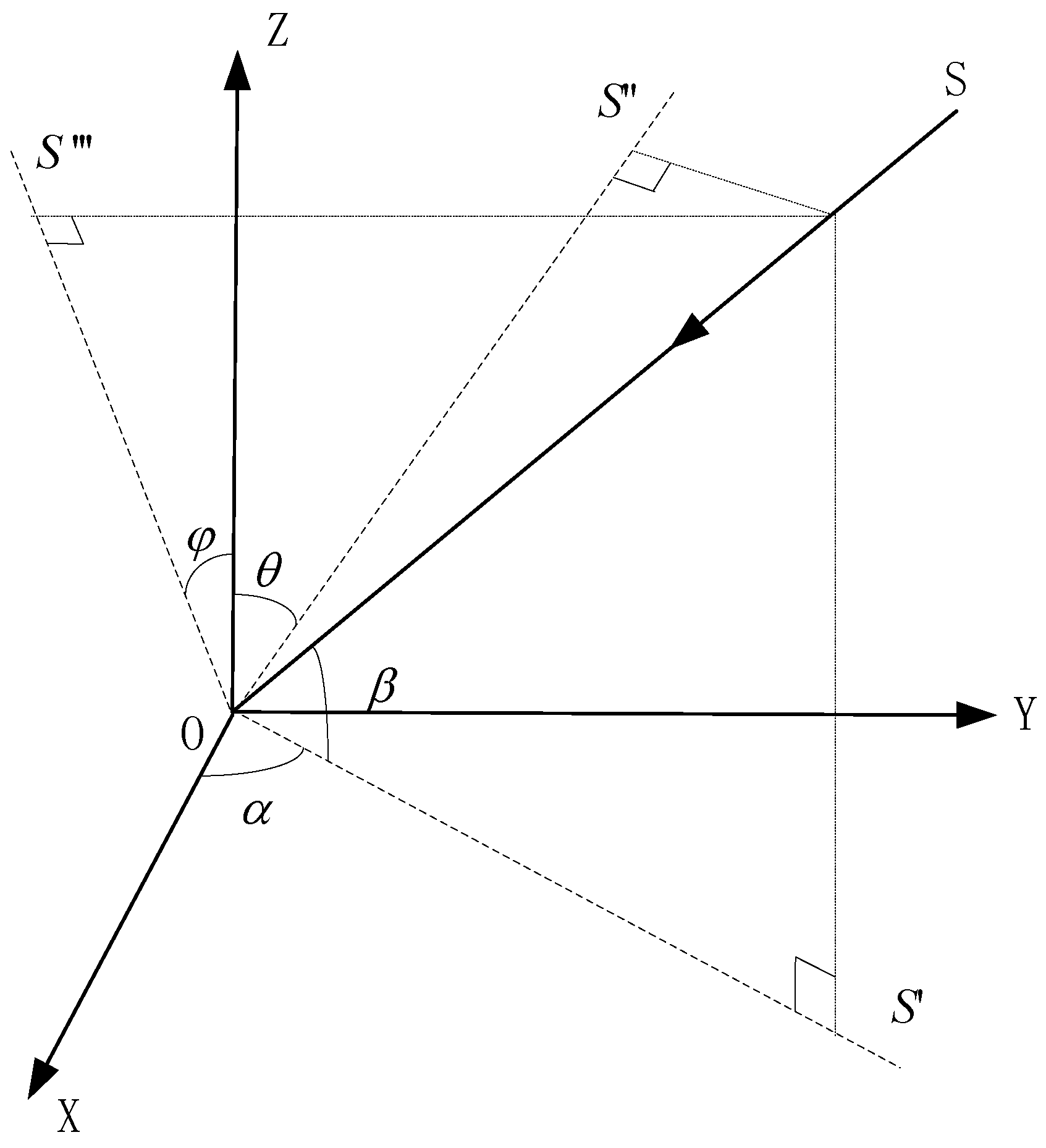
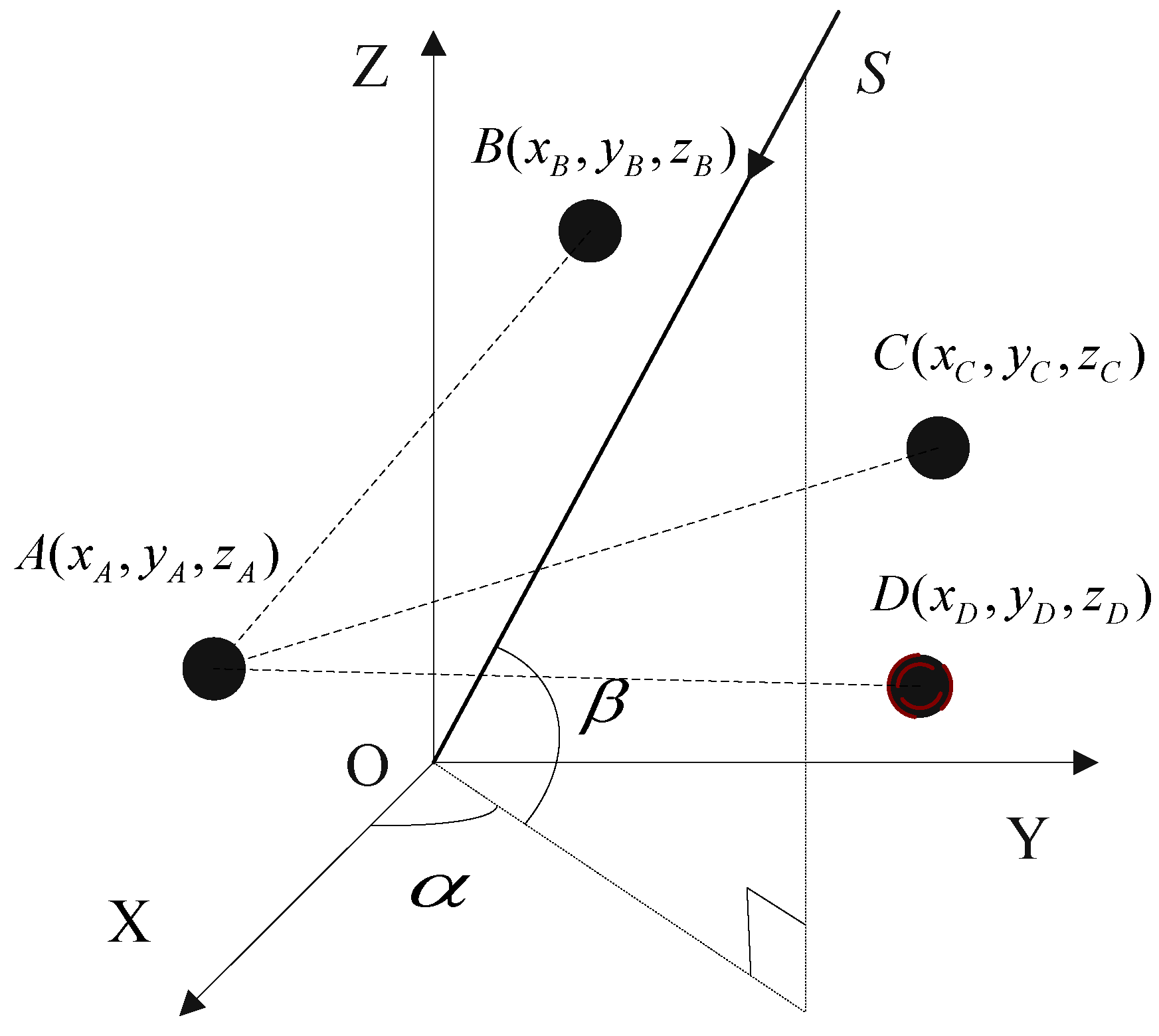
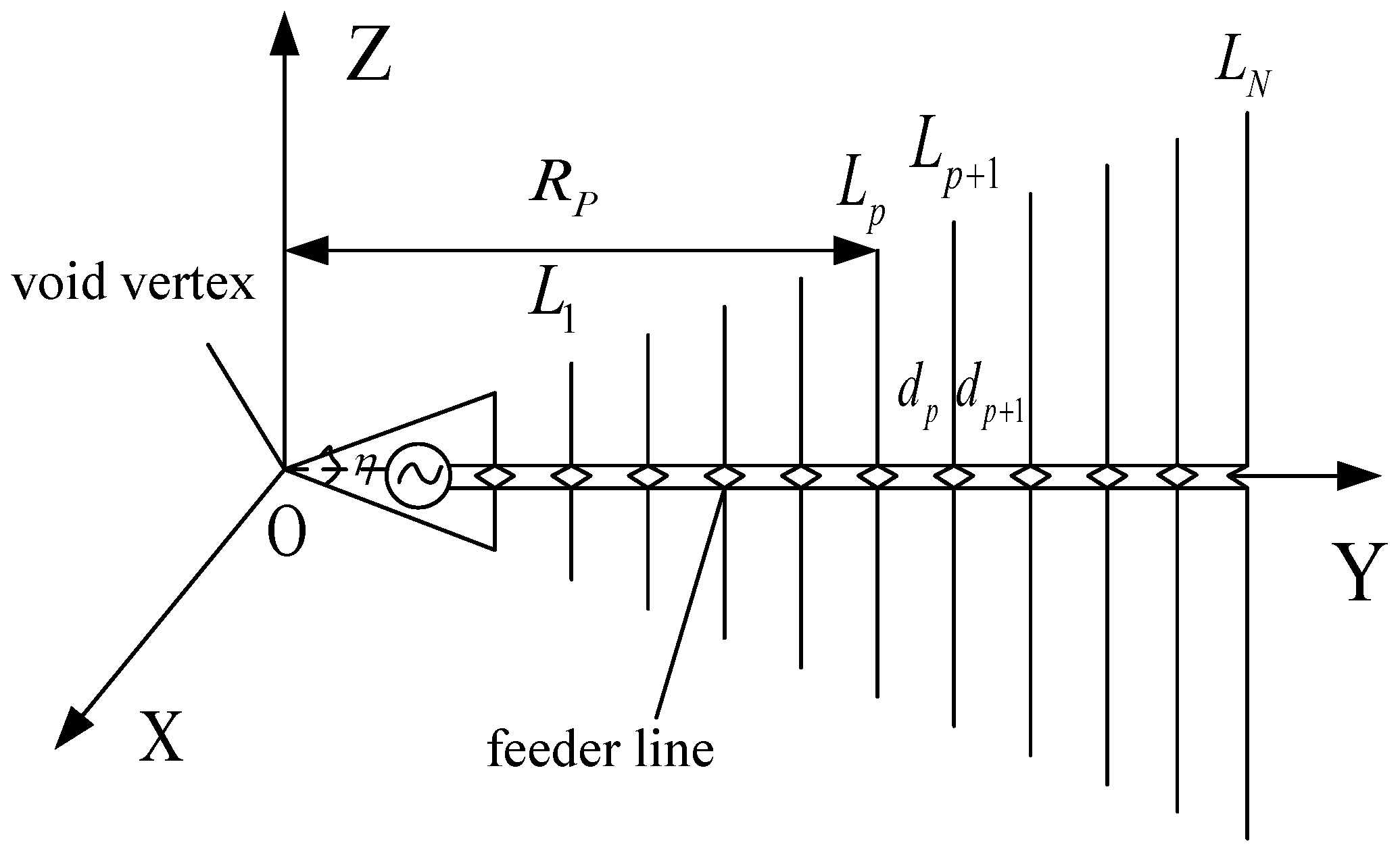
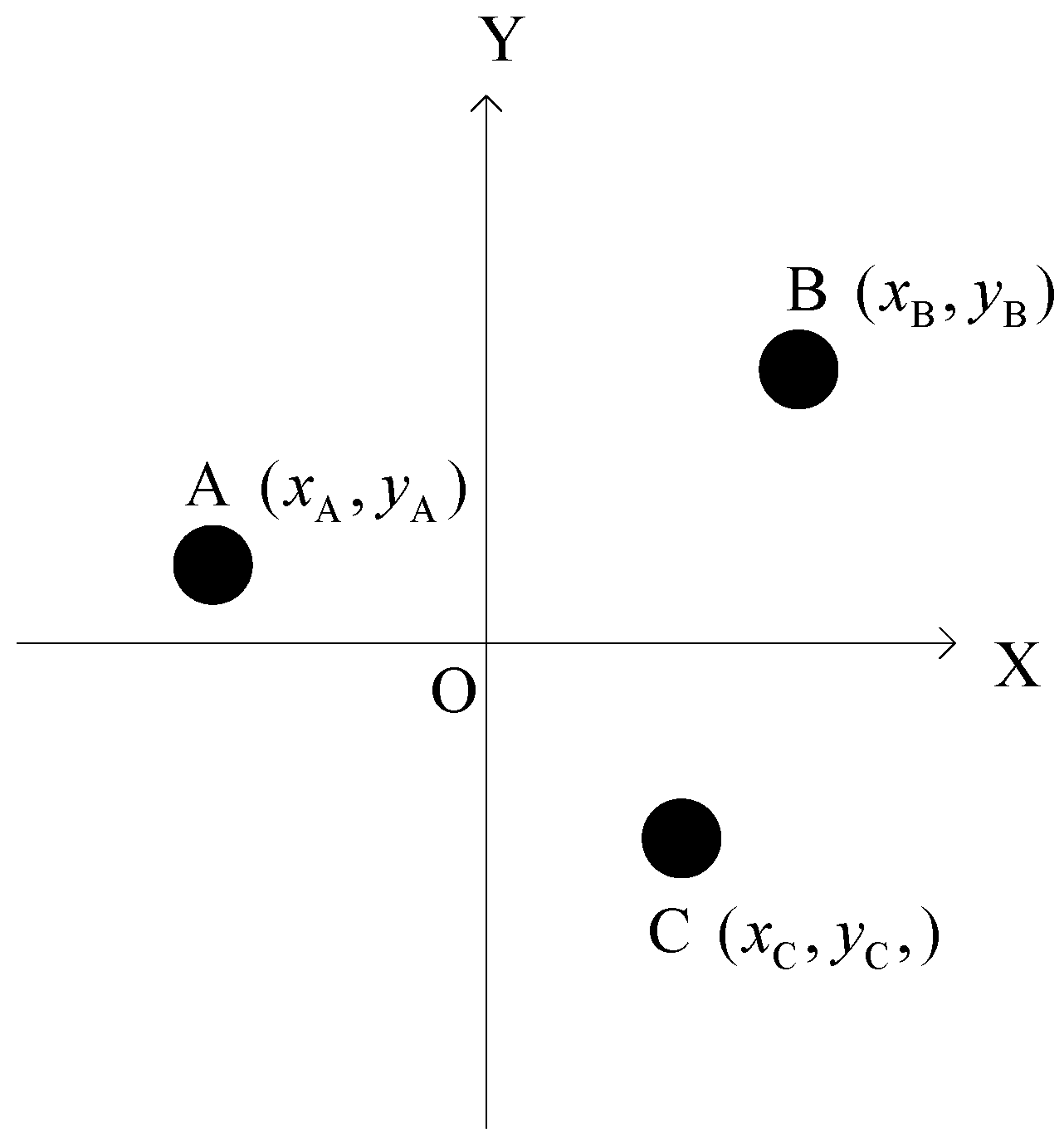
3.1. The Model of the Incident Signal

The direction finding of spatial Cartesian coordinate system is shown in Figure 3. $\overrightarrow{OS}$ is the incident signal of far-field. And $\overrightarrow{S^{\prime }O}$ is its projection in XOY plane. α and β stand for azimuth angle and elevation angle, respectively. Likewise, θ and $\phi$ represent course angle and pitching angle, respectively. According to the geometric, the relationship between α, β and θ, $\phi$ are expressed as:

$$tan\theta =cot\beta sin\alpha$$

(2)

$$tan\phi =cot\beta cos\alpha$$

(3)

As shown in Figure 3, θ and $\phi$ are generally used to control direction finding system in practice. According to Equations (4) and (5), if α and β are obtained by any algorithm, then θ and $\phi$ could be obtained easily.

Figure 3. Model of incident signal.

Figure 3. Model of incident signal.

The arbitrary baseline model is shown in Figure 4. A, B and C are three antenna elements placed in the space.

Assuming that the phase difference ambiguity does not exist and using simple geometric mathematic, the phase differences of the incident signal impinging on the antennas A, B, C can be represented as:

$${\varphi }_{\mathrm{AB}}^{}=\frac{2\pi }{\lambda }[(x_{\mathrm{B}}^{}-x_{\mathrm{A}}^{})·cos\beta ·cos\alpha +(y_{\mathrm{B}}^{}-y_{\mathrm{A}}^{})·cos\beta ·sin\alpha +(z_{\mathrm{B}}^{}-z_{\mathrm{A}}^{})·sin\beta ]$$

(4)

$${\varphi }_{\mathrm{AC}}^{}=\frac{2\pi }{\lambda }[(x_{\mathrm{C}}^{}-x_{\mathrm{A}}^{})·cos\beta ·cos\alpha +(y_{\mathrm{C}}^{}-y_{\mathrm{A}}^{})·cos\beta ·sin\alpha +(z_{\mathrm{C}}^{}-z_{\mathrm{A}}^{})·sin\beta ]$$

(5)

$${\varphi }_{\mathrm{BC}}^{}=\frac{2\pi }{\lambda }[(x_{\mathrm{C}}^{}-x_{\mathrm{B}}^{})·cos\beta ·cos\alpha +(y_{\mathrm{C}}^{}-y_{\mathrm{B}}^{})·cos\beta ·sin\alpha +(z_{\mathrm{C}}^{}-z_{\mathrm{B}}^{})·sin\beta ]$$

(6)

where ${\varphi }_{\mathrm{AB}},{\varphi }_{\mathrm{AC}},{\varphi }_{\mathrm{BC}}$ stand for the phase differences respectively. In theory, the 2D-DOA could be acquired by solving any two of Equations (4–6).

Figure 4. Model of arbitrary baseline algorithm.

Figure 4. Model of arbitrary baseline algorithm.

3.2. The 2D Arbitrary Baseline Algorithm

The elements A, B, C are placed in the same plane as shown in Figure 5. $\left(x_i,y_i\right)$ represents the element’s coordinate (i = A, B, C). Z-axis coordinate is set to zero.

Figure 5. The position of antenna elements.

Figure 5. The position of antenna elements.

The phase difference ambiguity exists here. Under this condition, the phase differences of the incident signal impinging on the antennas A, B, C are simplified as:

$${\varphi }_{\mathrm{AB}}^{}+2k_1\pi =\frac{2\pi }{\lambda }[(x_{\mathrm{B}}^{}-x_{\mathrm{A}}^{})·cos\beta ·cos\alpha +(y_{\mathrm{B}}^{}-y_{\mathrm{A}}^{})·cos\beta ·sin\alpha ]$$

(7)

$${\varphi }_{\mathrm{AC}}^{}+2k_2\pi =\frac{2\pi }{\lambda }[(x_C^{}-x_{\mathrm{A}}^{})·cos\beta ·cos\alpha +(y_C^{}-y_{\mathrm{A}}^{})·cos\beta ·sin\alpha ]$$

(8)

$${\varphi }_{BC}^{}+2k_3\pi =\frac{2\pi }{\lambda }[(x_{\mathrm{B}}^{}-x_C^{})·cos\beta ·cos\alpha +(y_{\mathrm{B}}^{}-y_C^{})·cos\beta ·sin\alpha ]$$

(9)

where ${\mathrm{k}}_1,{\mathrm{k}}_2,{\mathrm{k}}_3=0,\pm 1,\pm 2···$. $tan\alpha$ is expressed as:

$$tan\alpha =\frac{({\varphi }_{\mathrm{AB}}^{}+2{\mathrm{k}}_1\pi )·(x_{\mathrm{C}}^{}-x_{\mathrm{A}}^{})-({\varphi }_{\mathrm{AC}}^{}+2{\mathrm{k}}_2\pi )·(x_{\mathrm{B}}^{}-x_{\mathrm{A}}^{})}{({\varphi }_{\mathrm{AC}}^{}+2{\mathrm{k}}_2\pi )·(y_{\mathrm{B}}^{}-y_{\mathrm{A}}^{})-({\varphi }_{\mathrm{AB}}^{}+2{\mathrm{k}}_1\pi )·(y_{\mathrm{C}}^{}-y_{\mathrm{A}}^{})}$$

(10)

It can be seen from Equation (10) that there is a mirror ambiguity of the incident signal. i.e., if $tan\alpha >0$, the incident signal may come from both the first and the third quadrants; else if $tan\alpha <0$, the incident signal may come from the other two quadrants. Fortunately, the actual direction where the incident signal comes from can be distinguished. As shown in Figure 5, if ${\varphi }_{\mathrm{AB}}^{}+2{\mathrm{k}}_1\pi >0$, the incident signal is from the first quadrant, otherwise the signal is from the third quadrant. So as the condition $tan\alpha <0$.

A group solution is obtained by solving any two of Equations (7–9) containing the ambiguous value. Assume there are n elements in the space, so there are $C_3^n$ combinations of antennas. In order to solve the phase ambiguity, several other combinations are considered. Because the real value exists in all combinations, which can be selected by comparing the ambiguous values contained in several combinations. Finally, the 2D-DOA of the incident signal is obtained.

It can be seen from Figure 5, the antennas of arbitrary baseline algorithm are still placed in the same plane. The crucial reason for that is the angle information contained in the trigonometric function i.e., Equations (4–6). We have to search the angle in the same way as MUSIC algorithm, because the analytical solution does not exist. In high frequency, the computation is enormous when so many ambiguous values exist. Therefore, it is difficult to implement in practice.

4. The 3D Arbitrary Baseline Algorithm

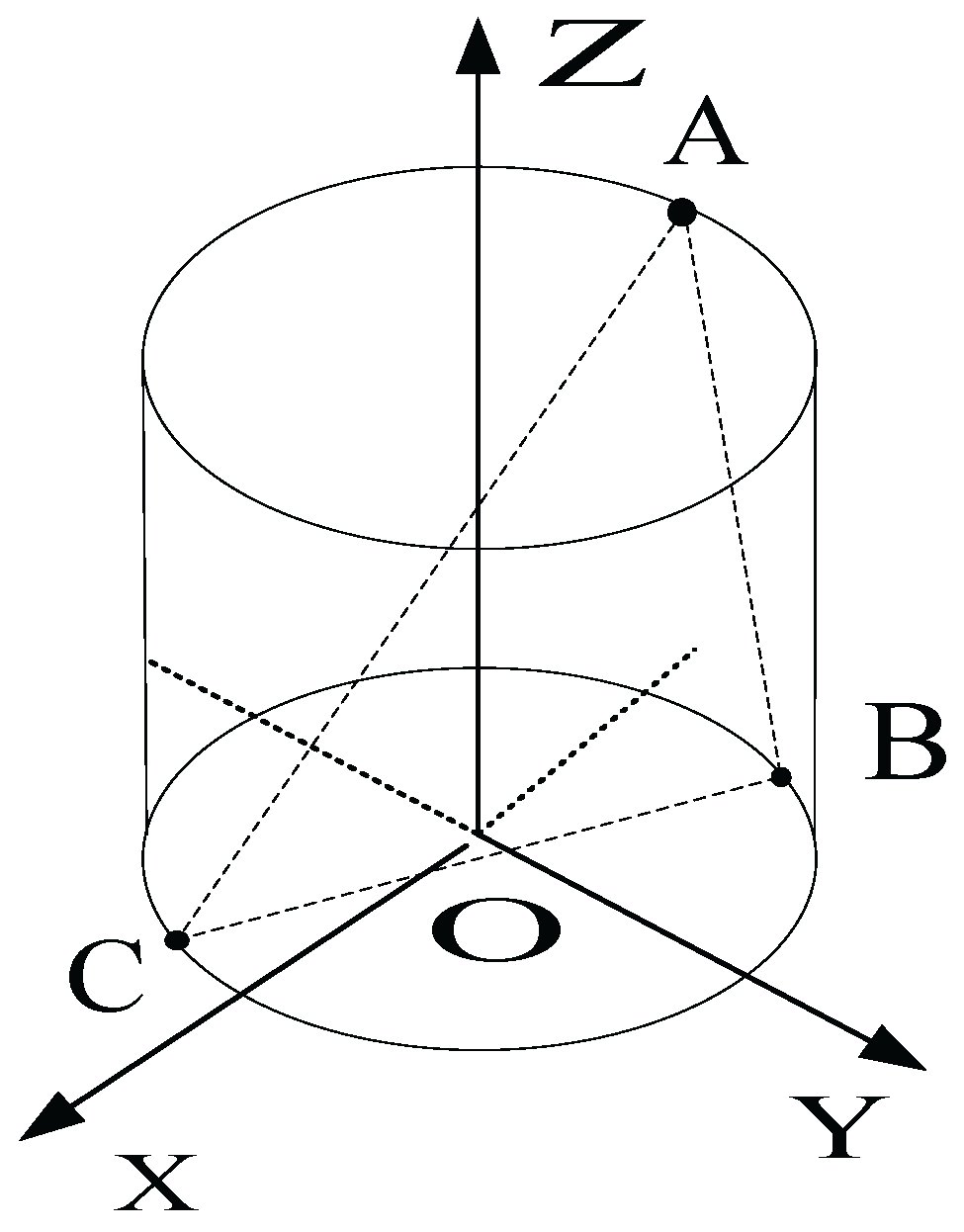
4.1. The Principle of 3D Arbitrary Baseline Algorithm

The direction finding principle for four antennas based on arbitrary baseline is shown in Figure 6. D is the fourth antenna placed in the space, and other conditions are the same as Figure 4.

Figure 6. Four antennas direction finding schematic.

Figure 6. Four antennas direction finding schematic.

The phase differences of the incident signal impinging on the four antennas A, B, C and D are represented respectively as follows:

$${\varphi }_{\mathrm{AB}}^{}+2k_1\pi =\frac{2\pi }{\lambda }[(x_{\mathrm{B}}^{}-x_{\mathrm{A}}^{})·cos\beta ·cos\alpha +(y_{\mathrm{B}}^{}-y_{\mathrm{A}}^{})·cos\beta ·sin\alpha +(z_{\mathrm{B}}^{}-z_{\mathrm{A}}^{})·sin\beta ]$$

(11)

$${\varphi }_{\mathrm{AC}}^{}+2k_2\pi =\frac{2\pi }{\lambda }[(x_C^{}-x_{\mathrm{A}}^{})·cos\beta ·cos\alpha +(y_C^{}-y_{\mathrm{A}}^{})·cos\beta ·sin\alpha +(z_C^{}-z_{\mathrm{A}}^{})·sin\beta ]$$

(12)

$${\varphi }_{\mathrm{AD}}^{}+2k_3\pi =\frac{2\pi }{\lambda }[(x_D^{}-x_{\mathrm{A}}^{})·cos\beta ·cos\alpha +(y_D^{}-y_{\mathrm{A}}^{})·cos\beta ·sin\alpha +(z_D^{}-z_{\mathrm{A}}^{})·sin\beta ]$$

(13)

Assuming ${\gamma }_1=cos\beta ·cos\alpha$, ${\gamma }_2=cos\beta ·sin\alpha$ and ${\gamma }_3=sin\beta$. Equations (11–13) can be expressed as the following matrix form:

$$\frac{\lambda }{2\pi }\left[\begin{array}{c}{\varphi }_{AB}+2k_1\pi \\ {\varphi }_{AC}+2k_2\pi \\ {\varphi }_{AD}+2k_3\pi \end{array}\right]=\left[\begin{array}{ccc}{x}_B-x_A& y_B-y_A& z_C-z_A\\ x_C-x_A& y_C-y_A& z_C-z_A\\ x_D-x_A& y_D-y_A& z_D-z_A\end{array}\right]\left[\begin{array}{c}{\gamma }_1\hfill \\ {\gamma }_2\hfill \\ {\gamma }_3\hfill \end{array}\right]$$

(14)

Therefore, the solution of Equation (14) is:

$$\left[\begin{array}{c}{\gamma }_1\\ {\gamma }_2\\ {\gamma }_3\end{array}\right]=\frac{\lambda }{2\pi }·{\left[\begin{array}{ccc}{x}_B-x_A& y_B-y_A& z_C-z_A\\ x_C-x_A& y_C-y_A& z_C-z_A\\ x_D-x_A& y_D-y_A& z_D-z_A\end{array}\right]}^{-1}\left[\begin{array}{c}{\varphi }_{AB}+2k_1\pi \\ {\varphi }_{AC}+2k_2\pi \\ {\varphi }_{AD}+2k_3\pi \end{array}\right]$$

(15)

There are two ways to solve α and β. The first is:

$$\begin{array}{c}\theta =arccos{\gamma }_3\hfill \\ \phi =arcsin\left(\frac{{\gamma }_1}{cos\left(\theta \right)}\right)or\phi =arcsin\left(\frac{{\gamma }_2}{sin\left(\theta \right)}\right)\hfill \end{array}$$

(16)

The second is:

$$\begin{array}{c}\phi =arctan\left(\frac{{\gamma }_2}{{\gamma }_1}\right)\hfill \\ \theta =arccos\left(\frac{{\gamma }_1}{cos\left(\phi \right)}\right)or\theta =arcsin\left(\frac{{\gamma }_2}{sin\left(\phi \right)}\right)\hfill \end{array}$$

(17)

The codomain of $sin\beta$ is $\left[0,1\right]$ in the first method, but ${\gamma }_3$ is larger than the codomain of $sin\beta$ at high frequency in practice. The real value of 2D-DOA can not be obtained because of so many ambiguous values at high frequency. As a result, the second method is selected in this paper. The codomain of $tan\alpha$ is $\left[-\infty ,+\infty \right]$. All azimuth angles can be covered, which will make it convenience to solve the phase ambiguity.

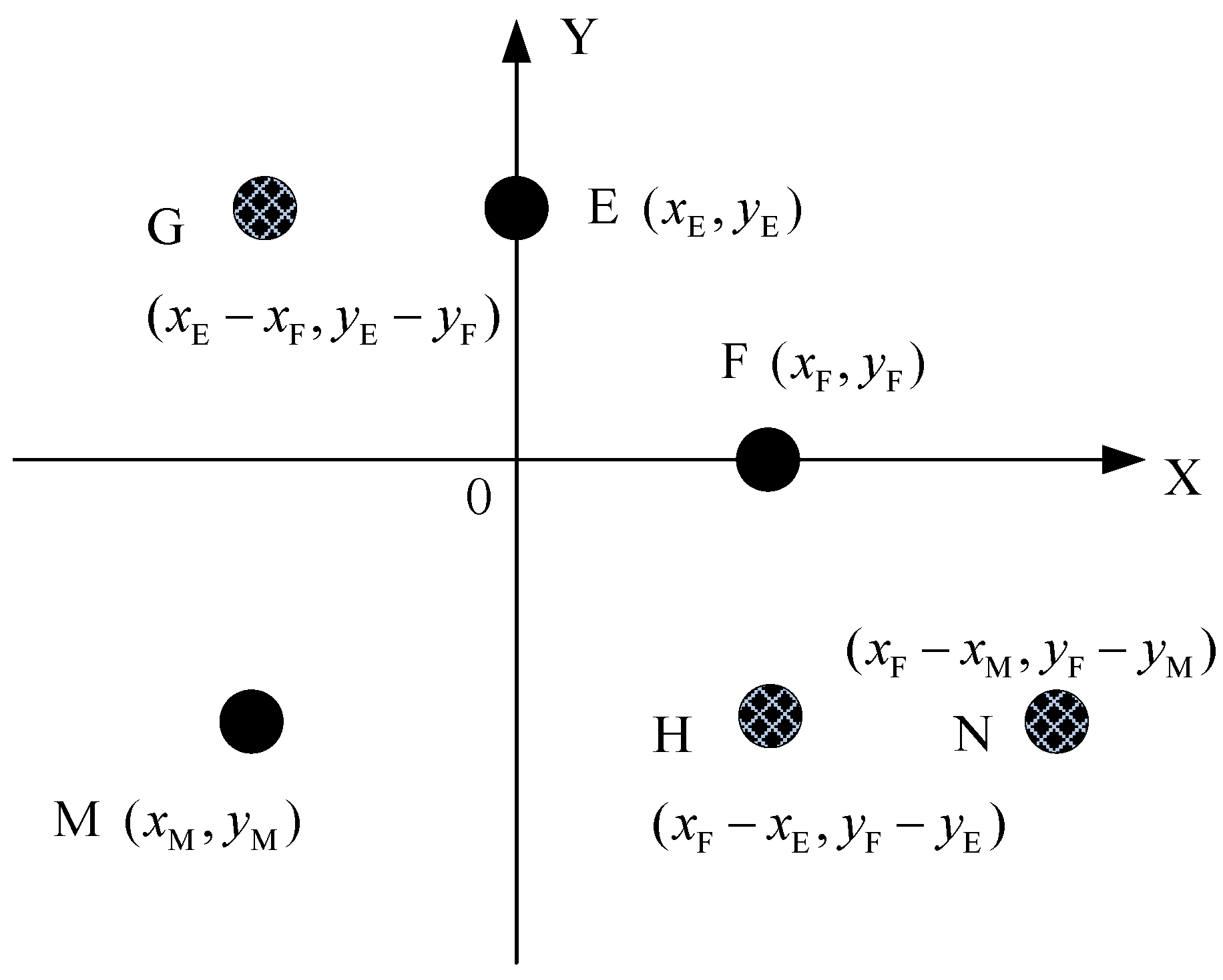
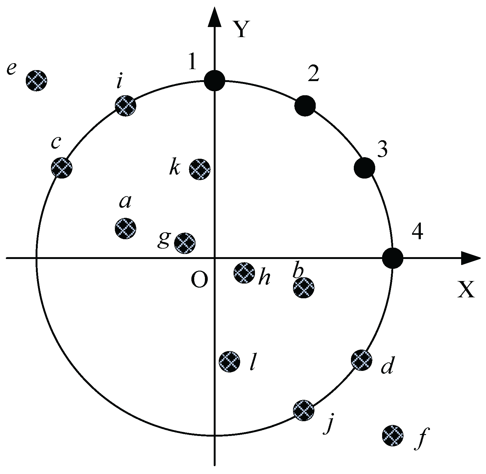
4.2. The Virtual Elements Based on Virtual Baseline

The virtual elements are constructed by the actual elements. Essentially, the virtual elements does not exist, which are constructed by the minus between different phase differences. The idea of virtual elements is that more information of the actual elements receive can be used for direction finding. The elements can be arranged more flexibility. If the length of the virtual baseline is short, the number of ambiguous values will be less than that of using actual baseline. Then the computational complexity of the rotation comparison method (It will be introduced in Section 4.3.) can reduce a lot.

In order to explain how to construct the virtual element in a simple way, we assume that the antennas E and F are placed in X-axis and Y-axis respectively. M is another antenna. The virtual element G and H constructed by E and F are shown in Figure 7. According to the principle of the arbitrary algorithm, the phase differences of M, F and E, F can be written as:

$${\varphi }_{\mathrm{FE}}^{}+2k_4\pi =\frac{2\pi }{\lambda }[(x_{\mathrm{E}}^{}-x_{\mathrm{F}}^{})·cos\beta ·cos\alpha +(y_{\mathrm{E}}^{}-y_{\mathrm{F}}^{})·cos\beta ·sin\alpha ]$$

(18)

$${\varphi }_{MF}^{}+2k_5\pi =\frac{2\pi }{\lambda }[(x_{\mathrm{F}}^{}-x_{\mathrm{M}}^{})·cos\beta ·cos\alpha +(y_{\mathrm{F}}^{}-y_{\mathrm{M}}^{})·cos\beta ·sin\alpha ]$$

(19)

Subtract Equation (19) from (18) from the left and right simultaneously, the phase difference between G and N is expressed as:

$$\begin{array}{c}{\varphi }_{\mathrm{GN}}^{}={\varphi }_{\mathrm{FE}}^{}-{\varphi }_{\mathrm{MF}}^{}+2k_6\pi \hfill \\ =\frac{2\pi }{\lambda }[(x_{\mathrm{E}}^{}+x_{\mathrm{M}}^{}-2x_{\mathrm{F}}^{})·cos\beta ·cos\alpha +(y_{\mathrm{E}}^{}+y_{\mathrm{M}}^{}-2y_{\mathrm{F}}^{})·cos\beta ·sin\alpha ]\hfill \end{array}$$

(20)

Equation (20) can be used instead of any two of Equations (11), (12) and (13) to solve Equation (15). Based on the virtual baseline method, all the information received by the elements should beused sufficiently.

Figure 7. Positions of the virtual elements. The black points represent the actual element (E, F and M); and the shadow points represent the virtual elements(G, H and N).

Figure 7. Positions of the virtual elements. The black points represent the actual element (E, F and M); and the shadow points represent the virtual elements(G, H and N).

4.3. The Solving Ambiguous Method Based on Rotation Comparison

For the principle of 3D arbitrary baseline algorithm, a group solution can be obtained from any four antennas placed in the space. Assuming there are n antennas, they should have $C_4^n$ combinations. The real 2D-DOA should be contained in each combination. Comparing the results with the multi-values of solving the equation constructed by each combination, the minimum error value among each combination would be defined as the real incident direction of the incident signal.

In order to clarify the principle of solving ambiguous problems intuitively, two combinations are used for direction finding. The result of the two combinations should be expressed as $\left[\begin{array}{cc}{\alpha }_{1i}& {\beta }_{1i}\end{array}\right]$ and $\left[\begin{array}{cc}{\alpha }_{2j}& {\beta }_{2j}\end{array}\right]$ respectively. The error value between two measurement results is defined as

$${\Delta }_{i,j}=\sqrt{{\left({\alpha }_{1i}-{\alpha }_{2j}\right)}^2+{\left({\beta }_{1i}-{\beta }_{2j}\right)}^2}$$

(21)

where $i,j=1,2,3···$, which the ith (or jth) ambiguous value respectively. The real 2D-DOA α and β are obtained by minimizing ${\Delta }_{i,j}$.

${\gamma }_1$ and ${\gamma }_2$ of Equation (16) or (17) are judged by positive or negative, the direction of the incident signal can be determined and thus the mirrored ambiguity is solved.

5. The Algorithm Based on Conformal Antenna

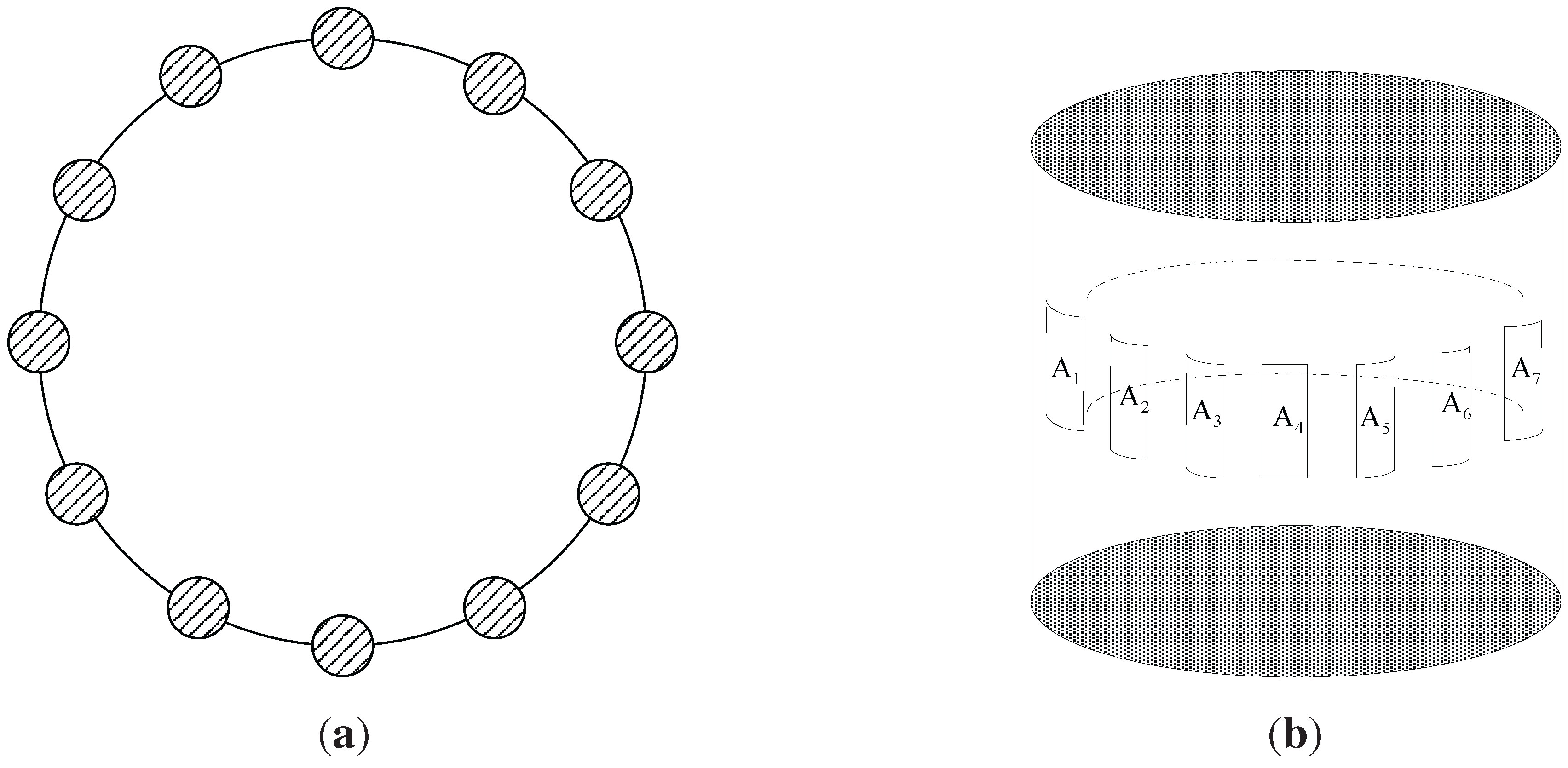
5.1. The Pre-Processing of Sub-Array Divided Technique

In order to eliminate the “shadow effect" caused by the metal structure, sub-array divided technique is used in this paper. The “shadow effect" means that when the incident signal comes from a special direction, not all antenna elements can receive the signal. The principle of sub-array divided technique is to ensure that at least one sub-array can receive the incident signal. For instance, on the cylindrical missile body, the sub-array divided technique should ensure that the coverage of each sub-array is more than $\pi /\phantom{\pi 2}2$. We can have an intuitive impression from Figure 8, which shows four elements arranged on the circumference in the first quadrant. The four black points are actual elements, and the twelve shadow points are virtual elements. Assuming there are n antennas, $A_2^n$ virtual elements can be constructed by the virtual baseline method. Both the actual elements and the virtual elements can be used for direction finding. The details for direction finding algorithm were described in Section 4.

Figure 8. Positions of the expanded virtual elements. The black points represent the actual elements (1–4); and the shadow points represent the virtual elements (a−l).

Figure 8. Positions of the expanded virtual elements. The black points represent the actual elements (1–4); and the shadow points represent the virtual elements (a−l).

5.2. The Algorithm Step

Virtual baseline algorithm combines with 3D arbitrary algorithm and 2D-DOA estimation is summarized as follows:

• The array antennas mounted on aircraft are arranged reasonably. Two combinations are selected in each sub-array for direction finding, the four antenna elements (including the virtual elements) constitute a combination;
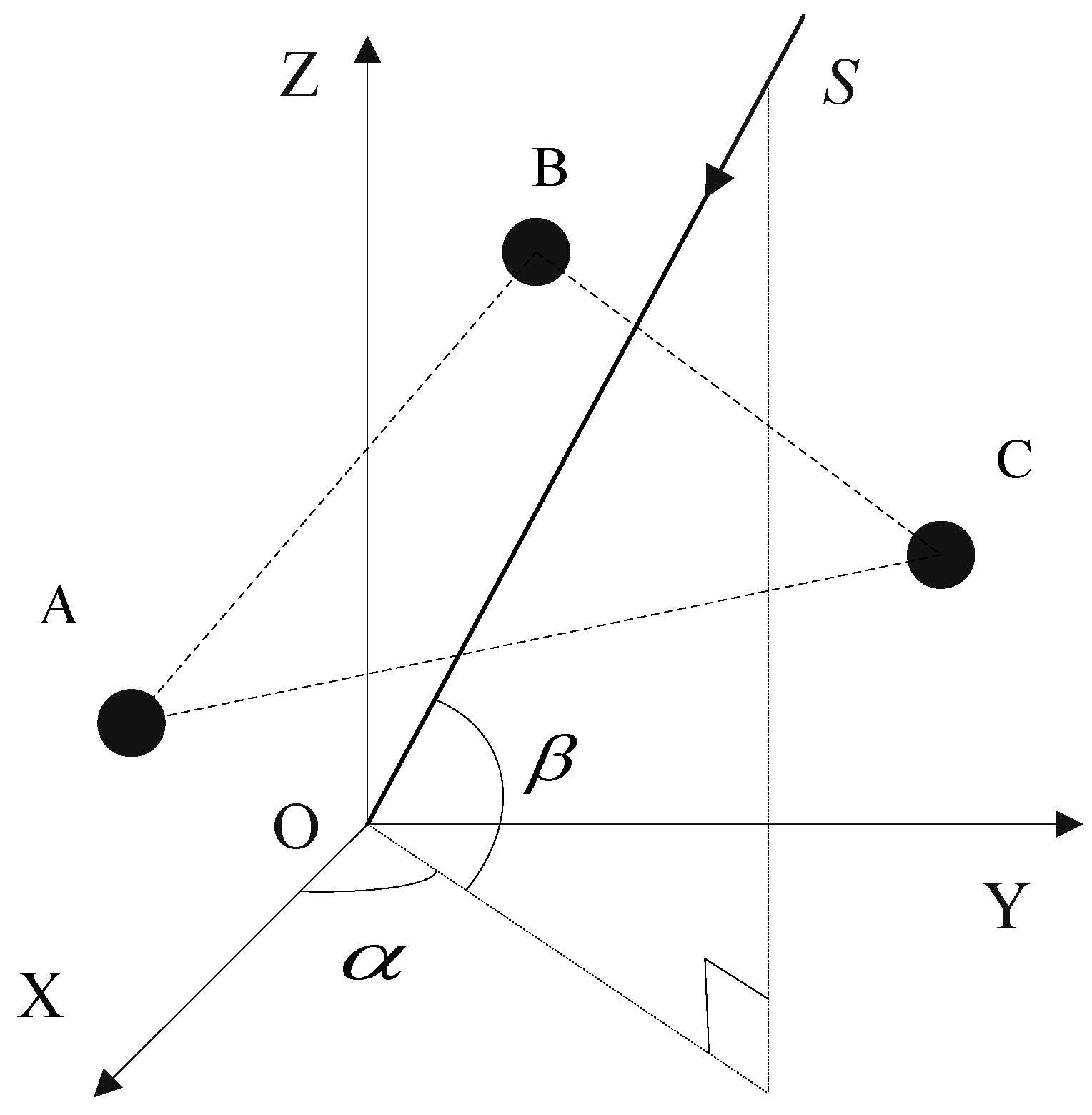
• The azimuth α and the elevation β can be obtained by solving Equations (16) or (17) of one combination. By checking whether ${\gamma }_1$ and ${\gamma }_2$ are positive or negative, the mirrored ambiguous problem can be solved. All values including ambiguous values are obtained, which will be recorded as the first solution;
• Apply the same procedure for another combination as step 2;
• According to Equation (20), the 2D-DOA of the incident signal can be obtained;
• Comparing the 2D-DOA of each sub-array (There is a greater difference between the error angle and the real angle due to the “shadow effect”), the closest value of each sub-array’s 2D-DOA is regarded as the real value, and the average value is calculated. Using transformation Equations (2) and (3), the course angle θ and pitching angle $\phi$ can be obtained finally.

6. The Analysis of Direction Finding Error

In this section, the direction finding error is derived in order to clarify the factors that affect the performance of direction finding. For simplicity, three elements are arranged on the surface of a cylinder as shown in Figure 9.

Figure 9. The model of antenna placement.

Figure 9. The model of antenna placement.

The cylindrical coordinate is adopted here. The transform from Cartesian coordinate system to cylindrical coordinates system can be expressed as

$$x_i=r·cos{\varphi }_i,y_i=r·sin{\varphi }_i,z_i=z_i(i=\mathrm{A},\mathrm{B},\mathrm{C})$$

(22)

where r stands for the radius of the antenna plate; ${\varphi }_i$ is angle between each element’s projection on the XOY plane and X-axis. Differentiating the two sides of Equations (4) and (5), they can be expressed as:

$$\begin{array}{c}\Delta {\varphi }_{AB}=\frac{2\pi }{\lambda }\left[-(x_B-x_A)sin\alpha +(y_B-y_A)cos\alpha \right]cos\beta \Delta \alpha \hfill \\ -\frac{2\pi }{\lambda }\left[-(x_B-x_A)sin\beta cos\alpha +(y_B-y_A)sin\beta sin\alpha -(z_B-z_A)cos\beta \right]\Delta \beta \hfill \end{array}$$

(23)

$$\begin{array}{c}\Delta {\varphi }_{AC}=\frac{2\pi }{\lambda }\left[-(x_C-x_A)sin\alpha +(y_C-y_A)cos\alpha \right]cos\beta \Delta \alpha \hfill \\ -\frac{2\pi }{\lambda }\left[-(x_C-x_A)sin\beta cos\alpha +(y_C-y_A)sin\beta sin\alpha -(z_C-z_A)cos\beta \right]\Delta \beta \hfill \end{array}$$

(24)

Based on Equation (22), $\Delta \alpha$ and $\Delta \beta$ can be represented as:

$$\Delta \alpha =\frac{m}{n}$$

(25)

where

$$\begin{array}{c}m=\left[(x_C-x_A)cos\alpha +(y_C-y_A)sin\alpha \right]\Delta {\varphi }_{AB}-\hfill \\ \left[(x_B-x_A)cos\alpha +(y_B-y_A)sin\alpha \right]\Delta {\varphi }_{AC}\hfill \end{array}$$

(26)

$$\begin{array}{c}n=\frac{2\pi }{\lambda }\left\{z_{\mathrm{A}}cot\beta \left[sin({\psi }_{\mathrm{B}}-\alpha )-sin({\psi }_{\mathrm{C}}-\alpha )\right]+\right.\hfill \\ \left.(x_C-x_A)(y_B-y_A)-(x_B-x_A)(y_C-y_A)\right\}cos\beta \hfill \end{array}$$

(27)

and

$$\Delta \beta =\frac{o}{p}$$

(28)

$$\begin{array}{c}o=\left[(y_B-y_A)cos\alpha -(x_B-x_A)sin\alpha \right]\Delta {\varphi }_{AC}-\hfill \\ \left[(y_C-y_A)cos\alpha -(x_C-x_A)sin\alpha \right]\Delta {\varphi }_{AB}\hfill \end{array}$$

(29)

$$\begin{array}{c}p=\frac{2\pi }{\lambda }\left\{z_{\mathrm{A}}cot\beta \left[sin({\psi }_{\mathrm{B}}-\alpha )-sin({\psi }_{\mathrm{C}}-\alpha )\right]+\right.\hfill \\ \left.(x_C-x_A)(y_B-y_A)-(x_B-x_A)(y_C-y_A)\right\}sin\beta \hfill \end{array}$$

(30)

where $\Delta \alpha$ and $\Delta \beta$ are the errors of azimuth and elevation respectively; $\Delta {\varphi }_{AC}$ and $\Delta {\varphi }_{AB}$ represent the measure errors of ${\varphi }_{AC}$ and ${\varphi }_{AB}$ respectively. The average number of phase difference is N. Usually, it is reasonable to assume that $\Delta {\varphi }_{AC}=\Delta {\varphi }_{AB}\approx 1/\phantom{1\sqrt{N\times SNR}}\sqrt{N\times SNR}$ (here SNR stands for signal to noise ratio). Using cylindrical coordinates, Equations (25) and (28) can be represented as

$$\Delta \alpha =\frac{1}{\frac{2\pi }{\lambda }cos\beta \sqrt{N\times SNR}}\times \frac{e}{f}$$

(31)

$$e=cos({\varphi }_{\mathrm{C}}-\alpha )-cos({\varphi }_{\mathrm{B}}-\alpha )$$

(32)

$$\begin{array}{c}f=\left\{z_{\mathrm{A}}cot\beta \left[sin({\varphi }_{\mathrm{B}}-\alpha )-sin({\varphi }_{\mathrm{C}}-\alpha )\right]+\right.\hfill \\ \left.r\left[sin({\varphi }_{\mathrm{B}}-{\varphi }_{\mathrm{C}})+sin({\varphi }_{\mathrm{C}}-{\varphi }_{\mathrm{A}})+sin({\varphi }_{\mathrm{A}}-{\varphi }_{\mathrm{B}})\right]\right\}\hfill \end{array}$$

(33)

$$\Delta \beta =\frac{1}{\frac{2\pi }{\lambda }sin\beta \sqrt{N\times SNR}}\times \frac{g}{h}$$

(34)

$$g=sin({\varphi }_{\mathrm{C}}-\alpha )-sin({\varphi }_{\mathrm{B}}-\alpha )$$

(35)

$$\begin{array}{c}h=\left\{z_{\mathrm{A}}cot\beta \left[sin({\varphi }_{\mathrm{B}}-\alpha )-sin({\varphi }_{\mathrm{C}}-\alpha )\right]+\right.\hfill \\ \left.r\left[sin({\varphi }_{\mathrm{B}}-{\varphi }_{\mathrm{C}})+sin({\varphi }_{\mathrm{C}}-{\varphi }_{\mathrm{A}})+sin({\varphi }_{\mathrm{A}}-{\varphi }_{\mathrm{B}})\right]\right\}\hfill \end{array}$$

(36)

When $z_A$ is zero, the 3D model deteriorates into 2D model.

$$\Delta \alpha =\frac{1}{\frac{2\pi r}{\lambda }cos\beta \sqrt{N\times SNR}}·\frac{cos({\varphi }_{\mathrm{C}}-\alpha )-cos({\varphi }_{\mathrm{B}}-\alpha )}{[sin({\varphi }_{\mathrm{B}}-{\varphi }_{\mathrm{C}})+sin({\varphi }_{\mathrm{C}}-{\varphi }_{\mathrm{A}})+sin({\varphi }_{\mathrm{A}}-{\varphi }_{\mathrm{B}})]}$$

(37)

$$\Delta \beta =\frac{1}{\frac{2\pi r}{\lambda }sin\beta \sqrt{N\times SNR}}·\frac{sin({\varphi }_{\mathrm{C}}-\alpha )-sin({\varphi }_{\mathrm{B}}-\alpha )}{[sin({\varphi }_{\mathrm{B}}-{\varphi }_{\mathrm{C}})+sin({\varphi }_{\mathrm{C}}-{\varphi }_{\mathrm{A}})+sin({\varphi }_{\mathrm{A}}-{\varphi }_{\mathrm{B}})]}$$

(38)

It can be seen obviously from Equations (31) and (34) that the error of 3D is always bigger than that of 2D. For (25) and (28) of 2D array, it is known that $\Delta \alpha$ and $\Delta \beta$ become smaller as the SNR increases. i.e., Increasing SNR helps to improve the accuracy of direction finding. Also, $\Delta \alpha$ and $\Delta \beta$ become smaller as the frequency increases. As shown in Figure 3, the coverage of azimuth α belongs to $\left[0,2\pi \right]$ and β belongs to $\left[0,\pi /\phantom{\pi 2}2\right]$ . Because the sinusoidal trigonometric function is not monotonous from 0 to $2\pi$, it is not obvious to see how the changing of α affects the direction finding error in Equations (37) and (38). The sinusoidal trigonometric function is monotonous from 0 to $\pi /\phantom{\pi 2}2$. It can be seen that $\Delta \alpha$ becomes larger with β increases. However, $\Delta \beta$ becomes smaller with β increases.

7. Simulation Results

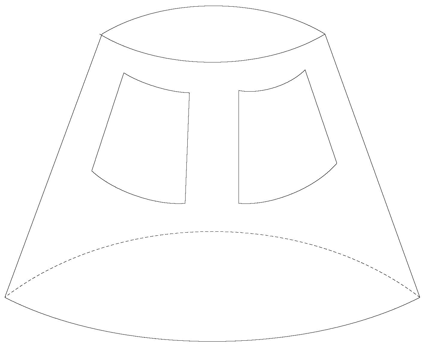
7.1. The Antenna Model

In order to verify the effectiveness of the proposed method, the arbitrary baseline algorithm based on the 2D array is compared with that based on 3D array in this section. Also, the arbitrary baseline algorithm is compared with MUSIC. The simulation results and analysis are elaborated as follows.

A twelve uniform circular array (UCA) is shown in Figure 10a. In each quadrant, four LPDA conformal antennas mounted on the cylindrical carrier are shown in Figure 10b. The approximate phase centers of arranged LPDAs are not in the same plane. The effects of mutual coupling and polarization mismatch are ignored. It can be seen in Figure 8 that the antennas 1–4 (four real elements and ten virtual elements in total) which can be divided into the first sub-array. And the antennas 2–5 can be divided into the second sub-array and so on. Using this sub-array divided technique, the 12-elements array can be divided into nine sub-arrays.

Figure 10. Antenna placement. (a) 2D array of the planar spiral antenna; (b) 3D array of LPDA conformal antenna.

Figure 10. Antenna placement. (a) 2D array of the planar spiral antenna; (b) 3D array of LPDA conformal antenna.

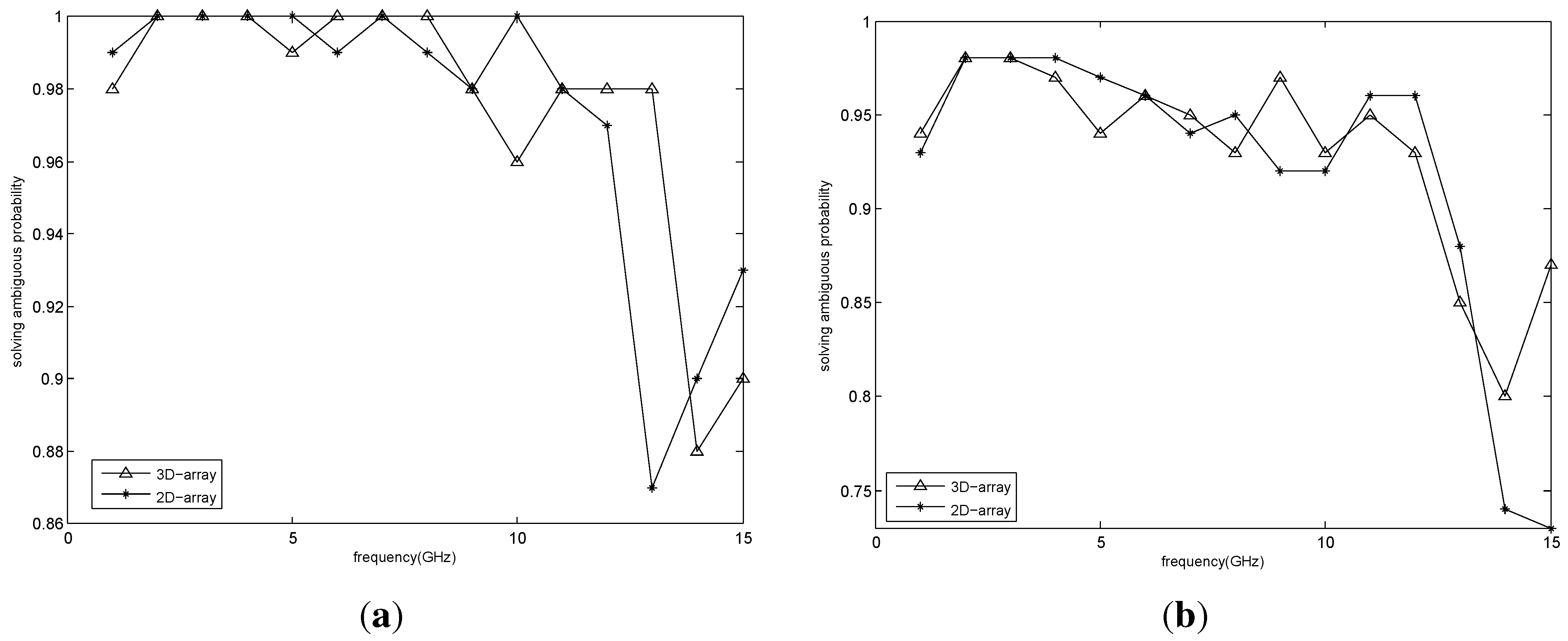
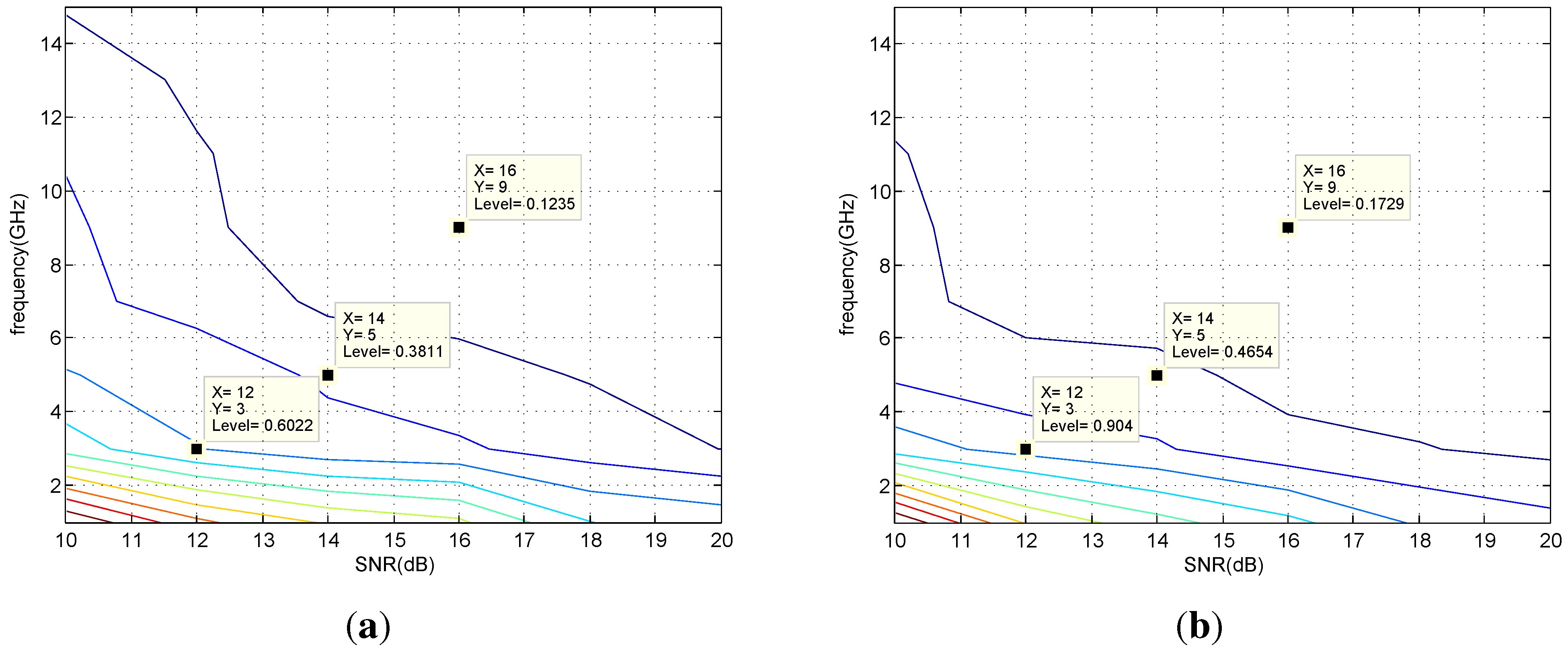
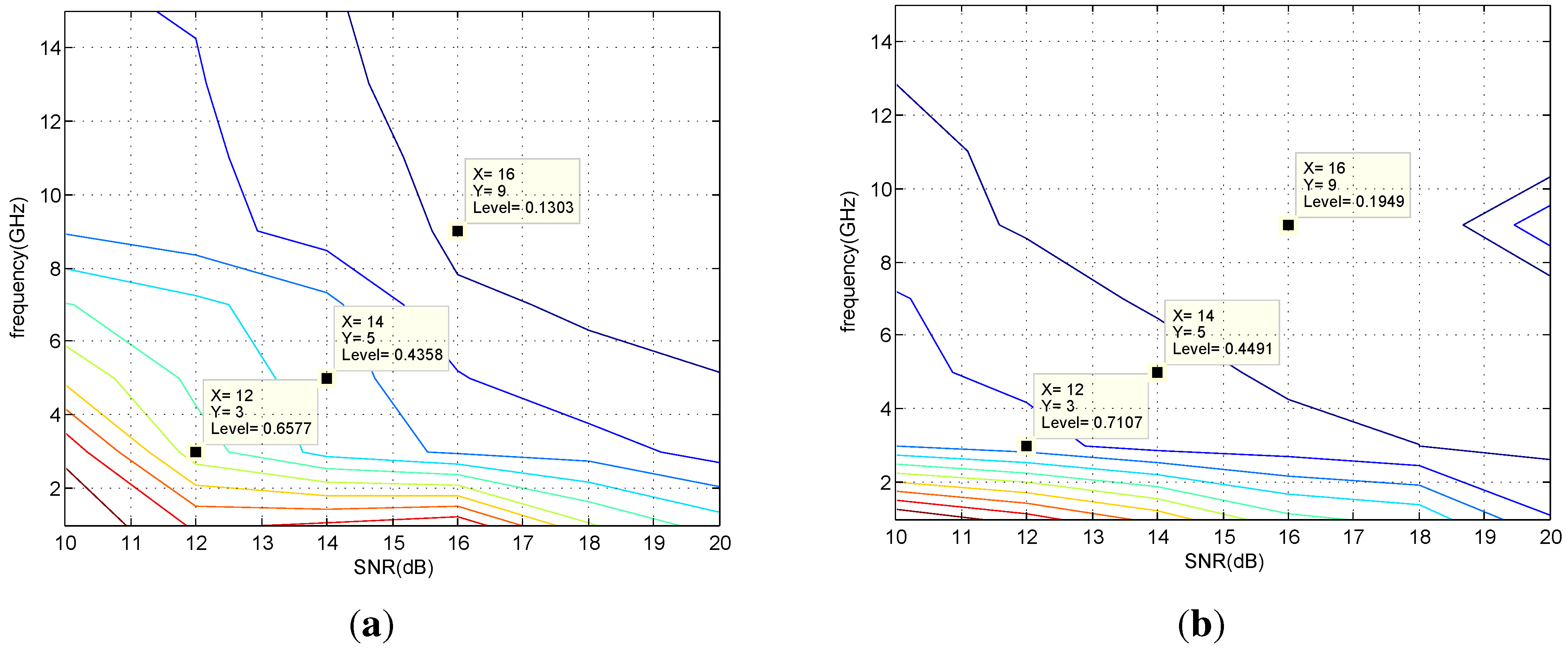
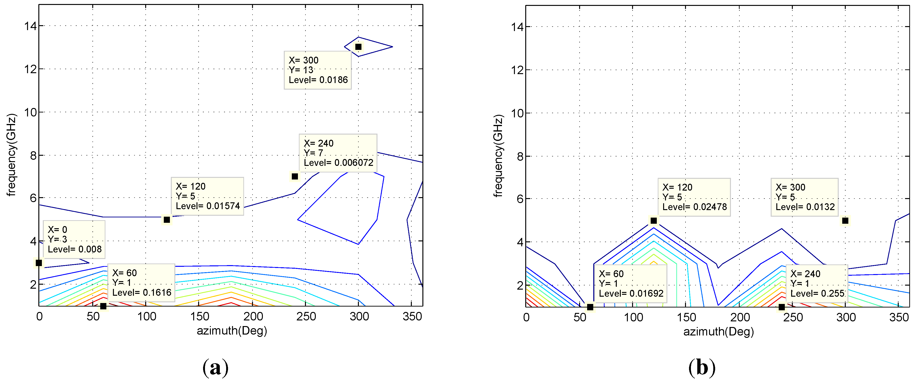
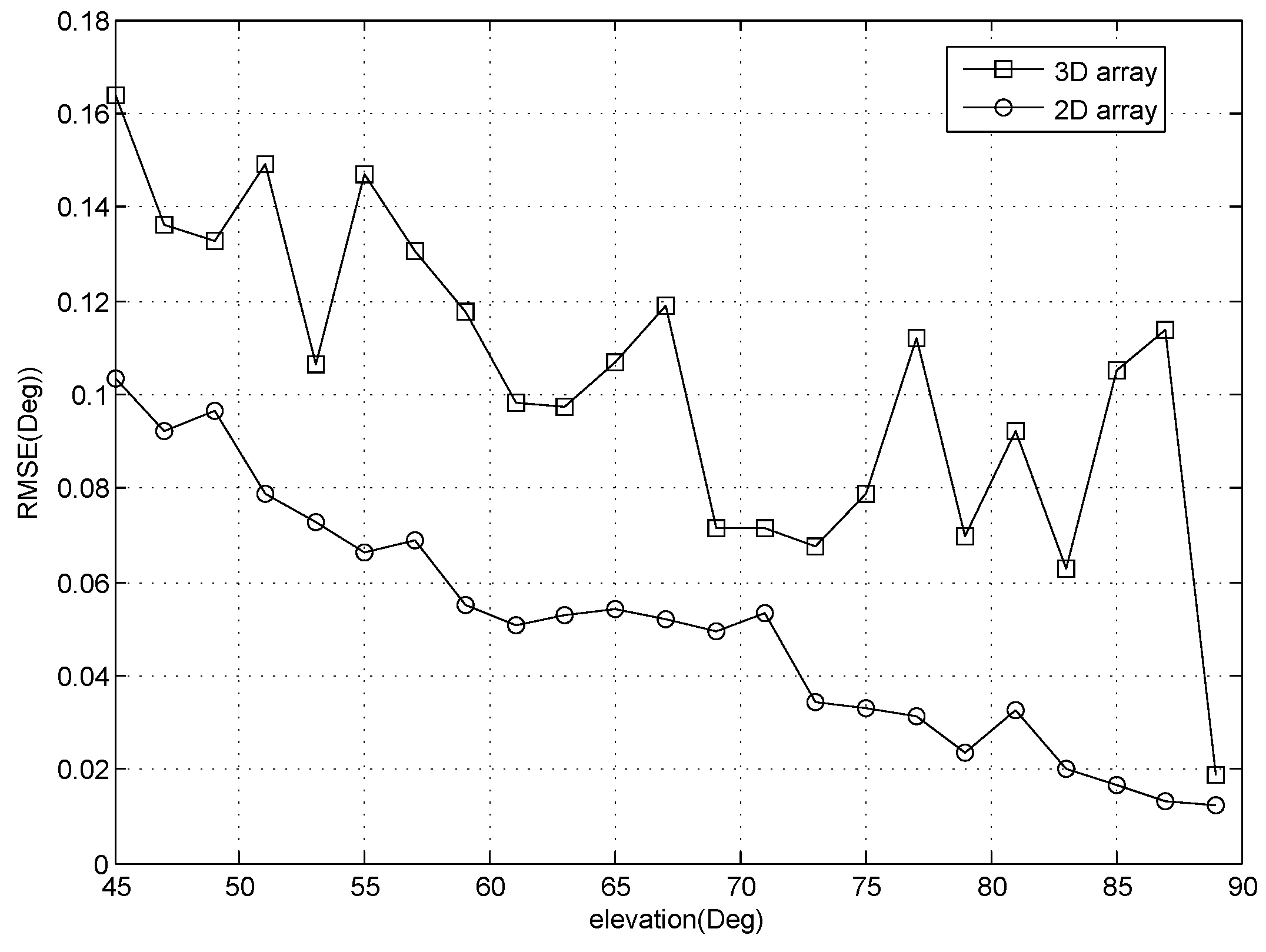
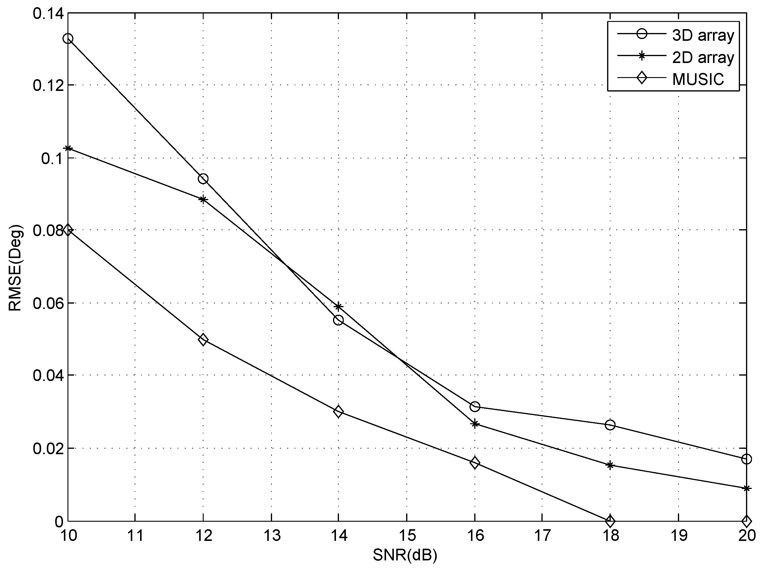
7.2. Simulation Results

The simulation conditions are: the radius of the antenna plate is 200 mm; the frequency range of incident signal is 1–15 GHz. In each experiment, only one incident signal is considered. The azimuth and elevation of the incident signal are $\left({45}^{\circ },{60}^{\circ }\right)$ and $\left({45}^{\circ },{80}^{\circ }\right)$ respectively.

Experiment 1 Comparison of two algorithms for solving ambiguous probability with different frequency. The incident angles of elevations are $\beta ={80}^{\circ }$ and $\beta ={60}^{\circ }$ respectively, and the SNR is 14 dB. The average number of phase difference is $N=20$, and 200 Monte-Carlo experiments are performed. The results of solving ambiguous probability are shown in Figure 11. It can be seen from Figure 11a that the incident signals are from 1 GHz to 15 GHz. The probability of solving ambiguous problem of both the 3D array and the 2D array is more than 86%. The high probability of solving ambiguity verifies that the scheme proposed in this paper can achieve no ambiguous direction finding in ultra-wideband.

Figure 11. Comparison of solving ambiguous probability at different frequencies. (a) $\beta ={80}^{\circ }$; (b) $\beta ={60}^{\circ }$.

Figure 11. Comparison of solving ambiguous probability at different frequencies. (a) $\beta ={80}^{\circ }$; (b) $\beta ={60}^{\circ }$.

As shown in Figure 11, the probability of solving ambiguity is decreasing with the frequency increasing. When we select actual value from the ambiguous values, the number of the ambiguous values at high frequency is enormous. The procedure gets more complicated and difficult which causes the behavior described above. It can be seen more intuitively in Equation (11). If the wavelength λ in the right of the equation becomes shorter, obviously the k in the left of the equation gets bigger and the number of ambiguous values increases.

Comparing Figure 11a with Figure 11b, it can be seen that the probability of solving ambiguity at $\beta ={60}^{\circ }$ is less than that at $\beta ={80}^{\circ }$. This is due to the fact that the incident signal is relatively further with the antenna boresight at $\beta ={60}^{\circ }$. The wave path difference between the antenna elements increases, which causes the ambiguous values of phase difference to increase. Thus the probability of solving ambiguity decreases at $\beta ={60}^{\circ }$.

Experiment 2 The comparison of root mean square error (RMSE) of two algorithms with respect to different frequencies and SNR. The elevation angles of the incident signals are $\beta ={80}^{\circ }$ and $\beta ={60}^{\circ }$, respectively, and the frequencies range from 1 GHz to 15 GHz. The average number of phase difference is $N=40$, and the results of 200 Monte-Carlo experiments are shown in Figure 12 and Figure 13. Figure 12 depicts the RMSE with 2D array, and Figure 13 depicts the RMSE with 3D array.

With the increase of SNR, both the RMSE of two arrays are reduced, which indicates that increasing SNR can improve the direction finding accuracy of the two arrays. Comparing Figure 12 with Figure 13, the RMSE of 3D array is slightly larger than that of 2D array at the same SNR. The result is consistent with the analysis of direction finding error as shown in Equation (28). The datatips in the contour plot reflect the viewpoint as mentioned above. This is because the virtual elements of 3D array use the addition and subtraction operations of the phase difference repeatedly. An example is shown in Equation (20). In order to clarify this issue, we assume that $\Delta {\varphi }_{FE}$ represents the measure error of ${\varphi }_{\mathrm{FE}}^{}$, and $\Delta {\varphi }_{MF}$ represents the measure error of ${\varphi }_{MF}^{}$. The error $\Delta {\varphi }_{GN}$ is equal to $\Delta {\varphi }_{FE}$ minus $\Delta {\varphi }_{MF}$: ${\varphi }_{\mathrm{GN}}^{}={\varphi }_{\mathrm{FE}}^{}-{\varphi }_{\mathrm{MF}}^{}$. Obviously, the virtual baseline method can affect the direction finding accuracy. It can be seen that RMSE at $\beta ={60}^{\circ }$ is larger than RMSE at $\beta ={80}^{\circ }$ with the reason being that the incident signal direction is relatively further when the antenna boresight is at $\beta ={60}^{\circ }$. The RMSE is affected by so many ambiguous values.

Figure 12. Comparison of RMSE of 2D array with respect to different frequency and SNR. (a) $\beta ={80}^{\circ }$; (b) $\beta ={60}^{\circ }$.

Figure 12. Comparison of RMSE of 2D array with respect to different frequency and SNR. (a) $\beta ={80}^{\circ }$; (b) $\beta ={60}^{\circ }$.

Figure 13. Comparison of RMSE of 3D array with respect to different frequency and SNR. (a) $\beta ={80}^{\circ }$; (b) $\beta ={60}^{\circ }$.

Figure 13. Comparison of RMSE of 3D array with respect to different frequency and SNR. (a) $\beta ={80}^{\circ }$; (b) $\beta ={60}^{\circ }$.

Experiment 3 The RMSE comparison of two algorithms with respect to different frequencies and azimuths. The elevation angle of incident signal is $\beta ={80}^{\circ }$, and the frequencies range from 1 GHz to 15 GHz. The SNR is 20 dB, and the average number of phase difference is $N=40$. The result of 200 Monte-Carlo experiments is shown in Figure 14. It can be seen from Figure 14 that the RMSE of the two arrays at low frequency is larger than that at high frequency. The higher the frequency is, the lower the RMSE is, which is consistent with the analysis of errors in Section 6. The RMSE of 3D array is slightly larger than planar array at the same azimuth which is caused by the fact that virtual elements of 3D array use the addition and subtraction operations of the phase difference repeatedly.

Experiment 4 The RMSE comparison of two algorithms with respect to different elevation angles. The azimuth angle of incident signal is $\alpha ={45}^{\circ }$, and the frequency is 6 GHz. The elevation angles range from ${45}^{\circ }$ to ${90}^{\circ }$. Other conditions are the same as those in experiment 3. The simulation result is shown in Figure 15. Briefly, the direction finding error decreases when elevation angle increases. Also, the RMSE of the 3D array is larger than that of 2D array. The result is consistent with the analysis of errors.

Figure 14. Comparison of RMSE with respect to different frequency and azimuth. (a) 2D array; (b) 3D array.

Figure 14. Comparison of RMSE with respect to different frequency and azimuth. (a) 2D array; (b) 3D array.

Figure 15. Comparison of RMSE with different elevation.

Figure 15. Comparison of RMSE with different elevation.

Experiment 5 The RMSE and average CPU time comparison of two algorithms with MUSIC. The azimuth and elevation of incident signal is $\left({45}^{\circ },{80}^{\circ }\right)$ and the frequency is 8 GHz. The average number of phase difference N is 40, and the results of 200 Monte-Carlo experiments are shown in Figure 16. It can be seen that the RMSE of 3D array is slightly larger than that of 2D array. However, the MUSIC algorithm performs the best among all methods. This is because the MUSIC algorithm uses a spectrum peak searching technique with high accuracy.

The CPU time comparison of the three algorithms is shown in Table 1. The PC with Intel Core 3.4 GHZ, 16 GB RAM is used for simulation. The SNR is 20 dB, and the frequency of incident signal is 8 GHz. 100, 200 and 500 Monte-Carlo experiments are considered respectively. It can be seen that the algorithm of 2D array is the fastest and the MUSIC algorithm is the slowest. The algorithm of 3D array is in the middle of the two algorithms mentioned above. It is caused by the fact that the algorithm of 3D array spends a lot of time on the matrix inversion. However, the computation of the spectrum peak searching is tremendous in comparison with the two algorithms mentioned above. The power of the direction finding system is assumed to be $P_t$. For 100 independent Monte-Carlo experiments, the energy consumption of 2D array, 3D array and MUSIC algorithm are $0.54P_t$, $4.53P_t$ and $20.06P_t$, respectively. If the energy of the direction finding system is fixed, then the working time of the proposed algorithm of 2D and 3D is much longer than that of MUSIC. Thus, the proposed algorithm outperforms than MUSIC, which has a low energy consumption.

Figure 16. Comparison of RMSE with different elevation.

Figure 16. Comparison of RMSE with different elevation.

Table 1. The consuming time of three algorithms.

Algorithm	100	200	500
2D array	0.54 s	0.94 s	2.22 s
3D array	4.53 s	9.05 s	22.29 s
MUSIC	20.06 s	41.79 s	108.10 s

Table 1. The consuming time of three algorithms.

Algorithm	100	200	500
2D array	0.54 s	0.94 s	2.22 s
3D array	4.53 s	9.05 s	22.29 s
MUSIC	20.06 s	41.79 s	108.10 s

8. Conclusions

A novel direction finding algorithm with low computational complexity is proposed in this paper. By combining the characteristics of the virtual baseline, the proposed algorithm adopts the sub-array divided technique and matrix inversion to acquire the course angle and the pitching angle. Four antenna elements are used as a combination, the elements do not need to be placed in the same plane. The simulations results demonstrate that there is little differences between the conformal array and the planar array in solving ambiguous probability and the RMSE. The proposed algorithm is suitable for direction finding based on conformal antenna in ultra-wideband. If the energy consumption of the direction finding system is fixed, the number of the direction finding of the proposed algorithm is much larger than that of MUSIC. The proposed algorithm has low energy consumption, which means one direction finding experiment based on the proposed algorithm can be completed in a very short time. It is suitable for real-time application.

References

1. Tsui, K.M.; Chan, S.C. Pattern synthesis of narrowband conformal arrays using iterative second-order cone programming. IEEE Trans. Antennas Propag. 2010, 58, 1959–1970. [Google Scholar] [CrossRef] [Green Version]
2. Zhang, Y.; Wan, Q.; Huang, A.M. Localization of narrow band sources in the presence of mutual coupling via sparse solution finding. Prog. Electromagn. Res. 2008, 86, 243–257. [Google Scholar] [CrossRef]
3. Wang, X.; Zhang, M.; Wang, S.J. Practicability analysis and application of PBG structures on cylindrical conformal microstrip antenna and array. Prog. Electromagn. Res. 2011, 115, 495–507. [Google Scholar] [CrossRef]
4. Wang, J.J.; Zhang, Y.P.; Chua, K.M.; Lu, A.C.W. Circuit model of microstrip patch antenna on ceramic land grid array package for antenna-chip codesign of highly integrated RF transceivers. IEEE Trans. Antennas Propag. 2005, 53, 3877–3883. [Google Scholar] [CrossRef]
5. Asimakis, N.P.; Karanasiou, I.S.; Uzunoglu, N.K. Non-invasive microwave radiometric system for intracranial applications: A study using the conformal L-notch microstrip patch antenna. Prog. Electromagn. Res. 2011, 117, 83–101. [Google Scholar] [CrossRef]
6. Comisso, M.; Vescovo, R. Fast co-polar and cross-polar 3D pattern synthesis with dynamic range ratio reduction for conformal antenna arrays. IEEE Trans. Antennas Propag. 2013, 61, 614–626. [Google Scholar] [CrossRef]
7. Milligan, T. More applications of euler rotation. IEEE Trans. Antennas Propag. Mag. 1999, 41, 78–83. [Google Scholar] [CrossRef]
8. Wang, B.H.; Guo, Y.; Wang, Y.L.; Lin, Y.Z. Frequency-invariant pattern synthesis of conformal array antenna with low cross-polarisation. IET Microw. Antennas Propag. 2008, 2, 442–450. [Google Scholar] [CrossRef]
9. Zou, L.; Lasenby, J.; He, Z.S. Beamformer for cylindrical conformal array of non-isotropic antennas. Adv. Electr. Comput. Eng. 2011, 1, 39–42. [Google Scholar] [CrossRef]
10. Zou, L.; Lasenby, J.; He, Z.S. Beamforming with distortionless co-polarisation for conformal arrays based on geometric algebra. IET Radar Sonar Navig. 2011, 5, 842–853. [Google Scholar] [CrossRef]
11. Boeringer, D.W.; Werner, D.H.; Machuga, D.W. A simultaneous parameter adaptation scheme for genetic algorithms with application to phased array synthesis. IEEE Trans. Antennas Propag. 2005, 53, 356–371. [Google Scholar] [CrossRef]
12. Li, W.T.; Hei, Y.Q.; Shi, X.W. Pattern synthesis of conformal arrays by a modified particle swarm optimization. Prog. Electromagn. Res. 2011, 117, 237–252. [Google Scholar] [CrossRef]
13. Xu, Z.; Li, H.; Liu, Q.Z. Pattern synthesis of conformal antenna array by the hybrid genetic algorithm. Prog. Electromagn. Res. 2008, 79, 75–90. [Google Scholar] [CrossRef]
14. Kong, L.Y.; Wang, J.; Yin, W.Y. A Novel dielectric conformal FDTD method for computing SAR distribution of the human body in a metallic cabin illuminated by an intentional electromagnetic pulse (Iemp). Prog. Electromagn. Res. 2012, 126, 355–373. [Google Scholar] [CrossRef]
15. Vaskelainen, L.I. Constrained least-squares optimization in conformal array antenna synthesis. IEEE Trans. Antennas Propag. 2007, 55, 859–867. [Google Scholar] [CrossRef]
16. Solimene, R.; Dell’Aversano, A.; Leone, G. Interferometric time reversal MUSIC for small scatterer localization. Prog. Electromagn. Res. 2012, 131, 243–258. [Google Scholar] [CrossRef]
17. Lee, J.H.; Jeong, Y.S.; Cho, S.W.; Yeo, W.Y.; Pister, K.S.J. Application of the Newton method to improve the accuracy of to a estimation with the beamforming algorithm and the MUSIC Algorithm. Prog. Electromagn. Res. 2011, 116, 475–515. [Google Scholar] [CrossRef]
18. Yang, P.; Yang, F.; Nie, Z.P. DOA estimation using MUSIC algorithm on a cylindrical conformal antenna array. IEEE Antennas Propag. Symp. 2007, 5299–5302. [Google Scholar] [CrossRef]
19. Yang, P.; Yang, F.; Nie, Z.P. DOA estimation with sub-array divided technique and interporlated esprit algorithm on a cylindrical conformal antenna array. Prog. Electromagn. Res. 2010, 103, 201–216. [Google Scholar] [CrossRef]
20. Qi, Z.S.; Guo, Y.; Wang, B.H. Blind direction-of-arrival estimation algorithm for conformal array antenna with respect to polarization diversity. IET Microw. Antennas Propag. 2011, 5, 433–442. [Google Scholar] [CrossRef]
21. Zou, L.; Lasenby, J.; He, Z. Direction and polarization estimation using polarized cylindrical conformal arrays. IET Signal Process. 2012, 6, 395–403. [Google Scholar] [CrossRef]
22. Si, W.J.; Wan, L.T.; Liu, L.T.; Tian, Z.X. Fast estimation of frequency and 2-D DOAs for cylindrical conformal array antenna using state-space and propagator method. Prog. Electromagn. Res. 2013, 137, 51–71. [Google Scholar] [CrossRef]
23. Liang, J.; Liu, D. Two L-shaped array-based 2-d DOAs estimation in the presence of mutual coupling. Prog. Electromagn. Res. 2011, 112, 273–298. [Google Scholar] [CrossRef]
24. Henault, S.; Podilchak, S.K.; Mikki, S.M.; Antar, Y.M.M. A methodology for mutual coupling estimation and compensation in antennas. IEEE Trans. Antennas Propag. 2013, 61, 1119–1131. [Google Scholar] [CrossRef]
25. Chen, D.; Cheng, X. Hydrostatic pressure sensor based on a gold-coated fiber Modal interferometer using lateral offset splicing of single mode fiber. Prog. Electromagn. Res. 2012, 124, 315–329. [Google Scholar] [CrossRef]
26. Yao, H.Y.; Chang, T.H. Experimental and theoretical studies of a broadband superluminality in fabry-perot interferometer. Prog. Electromagn. Res. 2012, 122, 1–13. [Google Scholar] [CrossRef]
27. Rengarajan, S.R. Reflectarrays of rectangular microstrip patches for dual-polarization dual-beam radar interferometers. Prog. Electromagn. Res. 2012, 133, 1–15. [Google Scholar] [CrossRef]
28. Schmieder, L.; Mellon, D.; Saquib, M. Interference cancellation and signal direction finding with low complexity. IEEE AES Syst. 2010, 46, 1052–1063. [Google Scholar] [CrossRef]
29. Kawase, S. Radio interferometer for geosynchronous-satellite direction finding. IEEE AES Syst. 2007, 43, 443–449. [Google Scholar] [CrossRef]
30. Sundaram, K.R.; Mallik, R.K.; Murthy, U.M.S. Modulo conversion method for estimating the direction of arrival. IEEE AES Syst. 2000, 36, 1391–1396. [Google Scholar]
31. Pace, P.E.; Wickershan, D.; Jenn, D.C. High-resolution phase sampled interferometry using symmetrical number systems. IEEE Trans. Antennas Propag. 2001, 49, 1411–1423. [Google Scholar] [CrossRef] [Green Version]
32. Doron, M.A.; Doron, E. Wavefield modeling and array processing. I. Spatial sampling. IEEE Trans. Signal Process. 1994, 42, 2549–2559. [Google Scholar] [CrossRef]
33. Goossens, R.; Bogaert, I.; Rogier, H. Phase-mode processing for spherical antenna arrays with a finite number of antenna elements and including mutual coupling. IEEE Trans. Antennas Propag. 2009, 57, 3783–3790. [Google Scholar] [CrossRef]
34. Doron, M.A.; Doron, E. Wavefield modeling and array processing. II. Algorithms. IEEE Trans. Signal Process. 1994, 42, 2560–2570. [Google Scholar] [CrossRef]
35. Goossens, R.; Rogier, H.; Werbrouck, S. UCA Root-MUSIC with sparse uniform circular arrays. IEEE Trans. Signal Process. 2008, 56, 4095–4099. [Google Scholar] [CrossRef]