Abstract
A deep belief network (DBN) is a powerful generative model based on unlabeled data. However, it is difficult to quickly determine the best network structure and gradient dispersion in traditional DBN. This paper proposes an improved deep belief network (IDBN): first, the basic DBN structure is pre-trained and the learned weight parameters are fixed; secondly, the learned weight parameters are transferred to the new neuron and hidden layer through the method of knowledge transfer, thereby constructing the optimal network width and depth of DBN; finally, the top-down layer-by-layer partial least squares regression method is used to fine-tune the weight parameters obtained by the pre-training, which avoids the traditional fine-tuning problem based on the back-propagation algorithm. In order to verify the prediction performance of the model, this paper conducts benchmark experiments on the Movielens-20M (ML-20M) and Last.fm-1k (LFM-1k) public data sets. Compared with other traditional algorithms, IDBN is better than other fixed models in terms of prediction performance and training time. The proposed IDBN model has higher prediction accuracy and convergence speed.
1. Introduction
As a type of deep neural network, deep belief network (DBN) has a powerful predictive classification function. DBN is widely used in the field of prediction, such as recommendation systems. Nowadays, the Internet is developing rapidly, and it has become a big problem to obtain the desired resources from massive resources in a short period of time, and the recommendation system came into being. Currently, recommendation systems have been widely used on e-commerce platforms. With the continuous development of the Internet, more and more people are accustomed to conducting commodity transactions through the Internet. Recommendation systems can not only satisfy user interests, but also bring profits to enterprises. More and more e-commerce websites use recommendation systems, such as Amazon product recommendation, Douban music recommendation, news recommendation, etc. Therefore, using deep neural networks to improve the prediction accuracy of recommendation systems is the future development trend of the Internet.
In the field of deep learning, the internal structure of sample data is characterized by establishing a multi-level representation model, that is, by extracting high-level features layer by layer, so as to obtain a more abstract object representation [1]. The research of deep learning has a great impact in the field of artificial intelligence [2]. Deep models such as DBNs (deep belief networks) [3], convolutional neural networks (CNNs) [4] and recurrent neural networks (RNNs) [5] have been maturely applied to machine learning, pattern recognition, feature extraction and data mining. Inspired by deep learning and hierarchical representation, Professor Hinton proposed DBN as a generation model composed of multi-layer nonlinear neural units [6,7]. Through unsupervised learning and supervised learning, it can be applied to feature learning, prediction classification and image processing of sample data [8]. However, descriptions of how to determine the structure and size of the model are rarely seen in the literature. The network structure of DBN is generally derived from experience. If the network structure (including the number of neurons in each layer and the number of hidden layers) is set, it will not change, and doing so will bear a higher computational cost [9]. Shen et al. [10] determined the DBN structure through repeated manual experiments, but its model operation efficiency was low and the model performance was poor. However, the complexity of the network structure determines the ability to solve complex problems. Therefore, the more complex the network structure of DBN, the stronger the ability to solve complex problems. In the process of training DBN, the larger the number of neurons and the deeper the hidden layer, the more difficult the training and the longer the corresponding training time. At the same time, training errors are also accumulating, resulting in low accuracy of the model. In practical applications, DBN needs to build different network structures for different task scenarios. However, due to the lack of corresponding theoretical support and efficient training methods, researchers need to set network parameters based on experience, resulting in low model operation efficiency and poor model performance during the modeling process [11]. In order to prevent DBN from low training accuracy or data overfitting, it is very necessary for DBN to independently construct the best network structure. Therefore, how to independently construct the best network structure of DBN and obtain good performance has become a problem worth studying.
With the in-depth research on the DBN model, many researchers have proposed a variety of methods to improve the DBN model. Lopes et al. [12] proposed an adaptive step size technology to control the model learning rate, thereby improving the convergence of the contrastive divergence (CD) algorithm. Specifically, the learning rate of the model is controlled according to the update direction of the model parameters after iteration. Roy et al. [13] proposed to combine the effective features extracted by DBN with the sequence classifier of the recurrent neural network to improve the search performance of word hypotheses. Geng [14] et al. linked DBN with neuroscience and proposed a DBN based on glial cell mechanism to improve the performance of DBN for extracting data features. Although these improved deep belief networks (IDBNs) have good effects in many fields, if DBN can build a network model independently during the training process, it may greatly improve training efficiency. Palomo et al. [15] determined the neural network structure by self-organizing structure to improve the learning efficiency of neural network. However, when it comes to DBN, the self-organizing structure becomes very complicated [16].
Chen et al. [11] proposed a Net2Net technology to accelerate the experimental process by transferring knowledge from the previous network to a new, deeper and wider network. Inspired by this, transferring the important knowledge learned to the newly added substructure becomes an optimization method to determine the DBN structure. Afridi et al. [17] pointed out that transfer learning is the transfer of knowledge from the source task to the target task. He applied transfer learning to convolutional neural networks (CNNs). They transfer the feature layer knowledge learned from one CNN (source task) to another CNN (target task) to achieve transfer learning. It also shows that the knowledge of the source task will affect the performance of the target task. In fact, the idea of transfer learning can be applied to neural networks as a new learning framework to solve model training problems [11].
In view of the above analysis, we will propose a method based on knowledge transfer to construct the DBN network structure to determine the best model structure to improve training efficiency and model performance. First, initialize a basic three-layer structure, including the input layer (visible unit layer), hidden layer, and output layer. Through pre-training, the learned weight parameters are fixed. This is the first step of pre-training. Secondly, using the technology of knowledge transfer to transfer the weight parameters of the initial structure to a new and more complex structure, according to the expanded network rules, including expanding the network width and depth, independently constructs the best DBN network structure. At this point, the pre-training phase is completed. Next, the partial least square regression (PLSR) method is used to fine-tune the parameters of the IDBN structure. Qiao et al. [18] proposed that the back propagation (BP) algorithm has local minimum, long training time and gradient dispersion problems. He et al. [19] combined PLSR with the extreme learning machine, which overcomes the defects of the extreme learning machine itself, improves the prediction accuracy, and makes the model more robust. Therefore, using PLSR algorithm instead of BP algorithm can avoid the problems of BP algorithm. Finally, two types of prediction experiments are performed on the public data sets of Movielens-20M (ML-20M) and Last.fm-1k (LFM-1k). Compared with other fixed models, IDBN has higher prediction accuracy.
The structure of this paper is as follows: the first section introduces the related work on DBN, the second section introduces the improved deep belief network prediction model, including its construction algorithm, the third section gives the experimental process and the proof results, and finally the summary of this article.
2. Related Works
2.1. DBN
DBN is a probabilistic generative model composed of ordered stacking of multiple restricted Boltzmann machines (RBMs). The learning process of DBN is divided into two stages: unsupervised learning and supervised learning. First, the pre-training process of DBN uses an unsupervised layer-by-layer greedy method to obtain network weight parameters through the contrastive divergence (CD) algorithm; secondly, a supervised BP algorithm is used to fine-tune the weight parameters. An unsupervised learning process is from the input layer to the top layer of associative memory layer, while for the contrary, it is supervised learning process. The basic structure and learning process of DBN are shown in Figure 1.
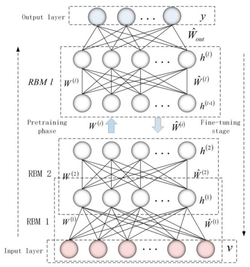
Figure 1.
The basic structure and learning process of deep belief network (DBN).
2.2. Unsupervised Learning Based on RBM
Unsupervised learning is a process of obtaining initial weights by training stacked RBMs layer by layer. The basic structure of RBM is shown in Figure 2. Given a set of states and a set of parameters , the energy function and joint probability distribution are defined as follows:
where is the partition function, is the visible layer unit vector, is the hidden layer unit vector, and is the weight matrix connecting the visible layer and the hidden layer, and are the bias vectors of the visible layer unit and the hidden layer unit, respectively. Calculate the marginal probability distribution about through the joint probability distribution:
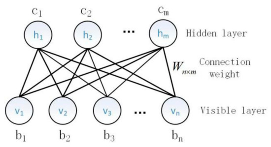
Figure 2.
RBM structure.
To update the weight parameters of RBM, the partial derivative with respect with respect to needs to be calculated. The parameter update rules are as follows:
where is the learning rate of the model. Since the second part of formula (4) contains the high computational complexity of the partition function, the CD algorithm is usually used to approximate . The training process of the CD algorithm only needs K steps (usually K = 1) Gibbs sampling to get good results. The sampling process of K-CD algorithm is shown in Figure 3.
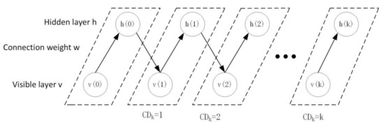
Figure 3.
K-CD algorithm sampling process.
In the sampling process, when the state of the visible layer unit is given, the activation probability of the -th hidden layer unit is:
where . Similarly, when the state of the hidden layer unit is given, the activation probability of the -th visible layer unit is:
Since the RBM unit state value is binary. Taking the hidden layer unit as an example, the state value of the hidden layer unit is determined by the random number , and the value state of is as follows:
In the unsupervised learning process, the greedy layer-by-layer training algorithm is used to train each layer of RBM from low to high. The hidden layer of each RBM is mapped to a different feature space. The higher the hidden layer, the more abstract features are obtained. The last hidden layer and the output layer of the top layer constitute an associative memory layer, which can correlate the optimal parameters of the remaining layers. Through unsupervised learning, DBN can obtain prior knowledge. In this paper, the initial weight obtained by pre-training is taken as an important knowledge in the process of knowledge transfer, which is the premise to determine the optimal network structure of DBN.
2.3. Supervised Learning Based on BP Algorithm
The main purpose of the BP algorithm is to fine-tune the initial weights obtained by pre-training to obtain the optimal weights. Assuming that is the actual output calculated by DBN through the initial weight, and is the corresponding target output, the loss function is defined as:
The weight is updated by gradient descent, so the weight update rule is:
where represents the number of iterations, and represents the learning rate.
Because of the gradient dispersion problem in BP algorithm, the gradient will become more and more sparse with the increasing number of hidden layers. The gradient dispersion problem is the main reason why the BP algorithm falls into a local minimum. Therefore, this paper adopts PLSR (partial least square regression) method to improve DBN convergence speed and fine-tuning accuracy.
3. Methods
In this section, the idea of transfer learning is applied to DBN to obtain the desired DBN. The basic idea of knowledge transfer is to transfer the knowledge learned from the initial network to a new network with a more complex structure. Its purpose is to accelerate the training of complex networks, realize the independent construction of the best network structure of DBN, improve the independent analysis ability of the model, and ensure that the model reaches the optimal state. Because DBN has strong feature detection and extraction capabilities, and can efficiently extract attribute data of different dimensions in input samples, DBN is often used for predictive classification problems.
In order to determine the optimal network structure of DBN and further improve and perfect the performance of DBN network, we propose a method for determining the network structure based on knowledge transfer. Knowledge transfer involves two operations: (1) expanding the network width, that is, adding a new hidden layer unit; (2) expanding the network depth, that is, adding a new hidden layer. In addition, the knowledge transfer process is carried out during the pre-training stage, and the optimal structure is fixed after completion. After the DBN structure is constructed, the PLSR algorithm is used instead of the BP algorithm to fine-tune the entire model. The DBN structure construction process is shown in Figure 4.
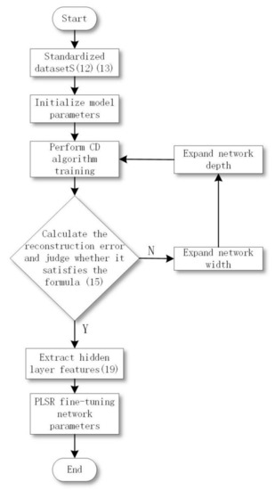
Figure 4.
DBN structure construction process.
3.1. DBN Structure Construction Method Based on Knowledge Transfer
This section provides the DBN self-construction pre-training stage based on knowledge transfer to improve the convergence speed and prediction performance of the model. The specific implementation steps are as follows:
S1: Standardize the data set. Including the analysis of the data set, classification, removal of noise, false data, feature standardization, etc. Standardize the data range to the [0,1] interval. Formula (12) is used for standardization processing.
where represents the sample point, represents the mean value of the j-th variable, and represents the standard deviation of . The formula for standard deviation is shown in (13). After preprocessing, the training samples are divided into three categories: training set , validation set and test set .
S2: Initialize model parameters. Initialize a basic DBN structure with a network depth of 2, including the visible layer (input layer), hidden layer, and output layer. In addition, there are strict requirements on the batch classification of experimental data, the setting of the number of initial hidden layer units, the setting of initial weights and biases, the learning rate and the number of iterations. Faced with a large number of data samples, it is necessary to classify samples for model training. Small batches of sample data can alleviate the computational burden. We set the batch of experimental data to 30 records per training. The number of initial hidden layer units is set to 40 for a single hidden layer unit. Initialize the connection weight, the visible layer and the hidden layer unit bias to N (0,0.1) random numbers conforming to the normal distribution. Learning rate is an important parameter, which not only affects the training efficiency of pre-training, but also affects the parameter update in the fine-tuning stage. We set the learning rate in the pre-training phase to 0.01, and the learning rate in the fine-tuning phase to 0.1. A reasonable number of iterations can effectively improve model performance. In order for each RBM to be fully trained, the number of iterations is set to 300.
S3: Pre-training (feature learning). In pre-training, each RBM uses the CD algorithm from bottom to top to complete the training and save the network parameters and . The purpose of model training is that DBN can reflect real data to the greatest extent after feature learning. This process can predict and classify data by extracting features and reducing dimensionality of high-dimensional data.
S4: Calculate the reconstruction error. In each layer of RBM, the reconstruction value of the input sample of the visible layer is obtained through the CD algorithm, and the reconstruction error is calculated by the difference between the reconstruction value and the initial input sample. If the reconstruction error reaches the minimum preset value, stop building and go to S7, otherwise, go to S5.
The definition of reconstruction error is as follows:
where n and m are the number of training samples and the number of features, respectively, and and are the original input and reconstruction input, respectively.
In order to prevent over-fitting of training data or large deviation of reconstruction data, while balancing the network training cost, when the difference between the two reconstruction errors is less than the preset value , the network stops expanding.
where represents the reconstruction error of the current -th layer, k represents the number of iterations, and represents the preset value. The selection of the preset value is the key to determining whether the network model structure is optimized. The preset value is too large to construct the optimal network structure; the preset value is too small, resulting in too many hidden layer units and deeper layers, which increases the computational burden. For the DBN classification prediction experiment, when we choose , the best network model structure is achieved.
S5: Expand the network width: add new hidden layer neurons. In order to expand the network width, we increase the number of hidden units each time to double the initial structure, and replace the initial weights and with twice the high-dimensional weight matrices and . The random mapping function is introduced below:
New weight matrices and are introduced to represent the weights of the new complex network, and give new weights:
It should be noted that the first n columns of the initial matrix are directly copied to , and the remaining n columns are created by selecting a random variable in . The weight of needs to be divided by the replication factor to adjust the weight in the network.
In fact, we introduce a random mapping function for each RBM layer. According to the transfer knowledge rules (17) and (18), the weight parameters learned in the first layer of the initial structure are repeatedly transferred to the corresponding layer of the new network structure. Reusing the learned knowledge is the essential idea of knowledge transfer. Figure 5 shows the process of expanding the network width.
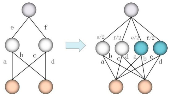
Figure 5.
Perform a step to expand the network width process.
S6: Expand the network depth: add a new hidden layer. Expanding the width of the network is to allow each hidden layer to learn richer features, and expanding the depth of the network means enhancing the ability of non-linear expression, which can fit more complex feature inputs. Specifically, it is to replace the last hidden layer of the current network with an identity module. The module has two layers, which are initialized to use identity mapping to retain the original function, that is to replace the two layers with the original hidden layer . The specific process of expanding the network depth is shown in Figure 6. Therefore, the number of hidden layer units in the new layer is initially set to be the same as the number of units in the lower layer, and can be further widened when the layer is widened. The new matrix initializes the identity matrix and is updated during training.
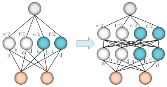
Figure 6.
Perform a one-step process of expanding the network depth.
The process of expanding the network depth has constraints on the activation function, that is, for all vectors , the activation function must satisfy: . This feature is suitable for linear rectification activation function (ReLU), but is invalid for sigmoid and tanh activation functions. However, for DBN, we can still use the network weights activated by sigmoid.
After completing step S6, go to S3.
S7: Complete the construction and fix the current structure parameters, and then enter the supervised fine-tuning stage.
3.2. PLSR-Based Fine-Tuning Algorithm
In the fine-tuning stage, the PLSR method is adopted. PLSR is a many-to-many modeling method. When multiple dependent variables and independent variables have multiple correlations, and the sample of observation data is small, the regression model established by PLSR has advantages that traditional classical regression analysis does not have. Although PLSR is a modeling method, it is also a supervised learning algorithm.
This paper uses the PLSR method to fine-tune the supervised parameters of the created DBN structure. Using the PLSR method to replace the BP algorithm can overcome the problems of the gradient-based supervised learning algorithm, such as local optimization and gradient dispersion. Since the PLSR method has no gradient calculation, this has also become the main advantage of PLSR. The fine-tuning steps based on PLSR are as follows:
S1: Extract the hidden layer feature vector matrix. After pre-training, the feature vectors of all hidden layers are extracted by using the input data X of the sample and the learned weights:
S2: Use PLSR to fine-tune network parameters. The PLSR modeling process is top-down, and PLSR equations are established every two layers, so as to obtain the output weight matrix optimized by the PLSR model.
The modeling process of target output and includes the following steps:
(1) Extract the first component
Knowing that both and are standardized, the first component is extracted from :
In Formula (20), is the first axis of , And =1, is the linear combination of the standardized variable .
Extract the first component from :
In Formula (21), is the first axis of , and = 1.
We require and to retain the maximum amount of information for and , respectively, and has the greatest ability to explain According to the principle of principal component analysis, it is actually required that the variance of and be the largest. Because the variance reflects the fluctuation of the data, the larger the variance, the more the original information can be reflected to the greatest extent. To maximize the variance between and , the correlation coefficient between and is the largest, that is, maximize the covariance between and , The formal description is:
Introduce the Lagrange multiplier to solve the optimization problem:
Calculate the partial derivatives of and , respectively, and get:
It can be derived:
It can be seen that is the eigenvector of and is the corresponding eigenvalue. Additionally, our objective function is to maximize , which is derived as follows:
That is, is the unit feature vector corresponding to the maximum feature value of . Similarly, is the unit eigenvector corresponding to the maximum eigenvalue of .
After obtaining the first axis and the components and can be obtained.
Then find the regression equations of and to respectively:
E and F in Equations (29) and (30) are the residual matrices of the two regression equations, respectively, and the regression coefficient vectors and are calculated using the least square method as:
(2) Extract the second component
Substituting the residual matrix and for and , and using the same method to calculate and , we get:
Similarly, and are the unit eigenvectors corresponding to the largest eigenvalues of and , respectively.
Therefore, the regression equation of E and F to is:
Then, calculate the second set of regression coefficients:
(3) By analogy, starting from step (3), the optimal number of principal components can be determined by minimizing the absolute error (AE), and the iteration can be stopped.
where is the expected output, and is the predicted output of extracting m principal components.
(4) Establish the PLSR equation and get the optimized output weight vector
After the value of m is determined, the PLSR equation of versus is finally obtained:
Equation (40) can be written in matrix form as follows:
Therefore, the PLSR model of and can be described as:
In Formula (42), is the prediction vector of , is the optimal number of components in the th layer, is the regression coefficient matrix of , is the transformation matrix. Therefore, the output weight matrix optimized by the PLSR model is:
Next, the PLSR modeling process is repeated every two layers from and to and . When the input layer and the first hidden layer are executed, the parameter fine-tuning phase ends, and all optimized weight matrices are obtained:
At this point, the independent construction process of DBN is complete.
4. Experiments
In order to verify the performance of the model proposed in this article, the prediction accuracy of the model is verified through two types of benchmark tests: (1) popularity prediction experiment based on time series; (2) rating classification prediction experiment based on user characteristics. The data set used in the experiment is a social network public data set: based on the music tag data set Last.fm-1k and based on the movie rating data set MovieLens-20M. In each experiment, the data set is divided into three categories: training set , validation set and test set , the corresponding data set length is , and . In addition, in the pre-training stage, the training set samples are used to determine the model initialization structure; in the network construction stage, the validation set samples are used to construct a knowledge transfer-based DBN structure; finally, the test set samples are used to test the DBN performance. In this paper, all experiments are run under the Window10_64bit operating system, the CPU model used is Intel Core i7-8550U 1.99GHZ, and the TensorFlow-1.10.1 deep learning framework was used to complete the simulation experiment. In this paper, root mean square error (RMSE) is used as the evaluation index of prediction effect, which is defined as follows:
where is the target output and is the predicted output. Our goal is to minimize RMSE and maximize model performance.
4.1. Datasets
Last.fm-1k (LFM-1k): this data set contains more than 1.91 million music listening events created by 1000 users (http://ocelma.net/MusicRecommendationDataset/index.html). Each listening event is defined as a four-tuple specified by user, timestamp, artist, and song name. In this experiment, the number of listening events of the track is used as the popularity index. The data set was acquired from February 2005 to June 2009.
Movielens-20M (ML-20M): this data set [20] is the most used public data set for recommender system testing. It contains 138,493 users who rated 27,278 movies, and the number of score records is 20 million. Each movie rating event includes user, movie, rating and time stamp information. Among them, the rating index range is 0.5–5.0. In this experiment, the number of times a movie gets ratings is used as a popularity index. The data set was acquired from January 1995 to March 2015.
4.2. Popularity Prediction Based on Time Series
The problem of time-series forecasting is a regression forecasting method that uses past and current time-series data for statistical analysis to predict future development trends. We define the popularity time series of the i-th item over a period of time as , where represents the popularity of the item i in the k-th sampling period. The goal of the prediction problem is to predict the popularity of item i in the next time period based on . The formal description is:
4.2.1. Validity Check
The number of hidden layer units of the initial structure of IDBN proposed in this paper is set to 40, and the number of iterations of the initial structure and the new structure are both 300, so that the DBN is fully trained, the learning rate k = 0.1, and the threshold of the stopping criterion is set to 0.03. Finally, in the LFM-1k data set through the independent construction of DBN, it is determined that the hidden layer is 3 layers, that is, the stopping criterion is met when the depth is 4. Therefore, the final IDBN structure was determined to be 20-80-160-160-1. In the ML-20M data set, the hidden layer is determined to be 4 layers, that is, the stop criterion is met when the depth is 5. Therefore, the final IDBN structure was determined to be 40-80-160-320-320-10. In order to compare the accuracy of the network depth determined by IDBN, the number of hidden layers of IDBN is sequentially increased. Table 1 shows the test results of IDBN at different depths. The number of neurons in each layer is the same as the IDBN model.

Table 1.
Improved deep belief network (IDBN) training results of different depths.
According to Table 1, as the network depth increases, the reconstruction error continues to decrease, but the running time is gradually increasing. For LFM-1k, when the depth is 4, the accuracy of the test data reaches the maximum; for ML-20M, when the depth is 5, the accuracy of the test data reaches the maximum, which further proves the correctness of the self-built algorithm.
In order to further show the effectiveness of IDBN prediction, a representative popularity sequence is selected from LFM-1k and ML-20M. Take the music “All I Need” as an example: select 1 month as the time interval, and use the number of comments obtained in each month as the popularity size to obtain the popularity time series. The popularity time series from 2006 to 2007 is used to train IDBN and predict the popularity in 2008. The forecast results are shown in Figure 7. Taking the movie "Forrest Gump" as an example, half a year is selected as the time interval, and the number of comments obtained in half a year is used as the popularity size to obtain the popularity time series. The popularity time series from 1996 to 2008 was used to train IDBN and forecast the popularity from 2009 to 2016. The forecast results are shown in Figure 8. Among them, the training result is the result after the implementation of PLSR fine-tuning. It can be seen from the experimental results that all time series points have been accurately predicted.
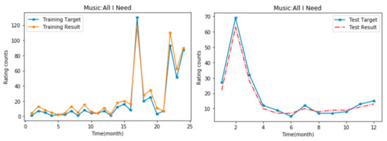
Figure 7.
Time series prediction of popularity of LFM-1k data set: left: training results; right: test results.
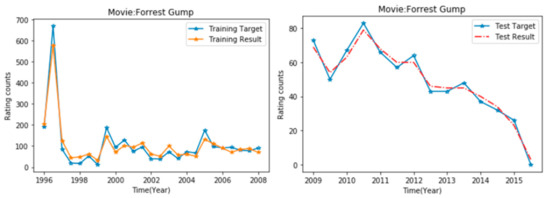
Figure 8.
Time series prediction of ML-20M data set popularity: left: training results; right: test results.
4.2.2. Predictive Performance Evaluation
In order to show the superiority of IDBN in the popularity time series, this paper compares the prediction performance of IDBN with the benchmark model. The comparison results are shown in Table 2, which includes RMSE and average training time. It should be pointed out that the parameters of all models in the table are selected through trial and error, so the performance is the best. Methods for comparison include self-organizing cascade neural network (SCNN) [21], new association model (NAM) [22], and other fixed structure models of DBN, such as CDBN, which is a DBN model with continuous input. The performance of auto-regressive integrated moving average (ARIMA)model is better than the support vector machine algorithm (SVR), because ARIMA is better at dealing with periodic time series as a classical time series analysis method. In the prediction problem based on time series, IDBN can continuously adjust the weight parameters in the model through independent construction and repair functions to obtain the improvement of prediction accuracy. Therefore, according to the experimental results, it can be concluded that IDBN can provide in the heat prediction experiment Better predictions.
Table 2.
Comparison results of popularity prediction based on time series.
4.3. Rating Classification Prediction Based on User Data
Because DBN has powerful feature detection and feature extraction functions, we use IDBN to perform efficient feature extraction on each user in the ML-20M dataset, and finally obtain the user’s rating prediction for the corresponding movie. Generally speaking, the rating range is [0.5, 5], reflecting the degree of preference from low to high, and each level represents a category. Therefore, the output layer of IDBN is a logistic regression classifier, and the number of neurons in the output layer is 10. The rating scale is shown in Table 3.
Table 3.
Rating scale.
4.3.1. Validity Check
After IDBN’s independent construction, the IDBN structure is finally determined: 40-160-160-160-160-10. After fine-tuning based on PLSR, test samples are used to verify whether the IDBN model can provide unbiased estimates. In the experiment, we randomly selected 100 users, and for each user, we obtained the actual ratings and predicted ratings of the users in the test sample. The experimental results are normalized. The test results are shown in Figure 9.
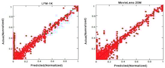
Figure 9.
Comparison of actual ratings and predicted ratings.
According to the experimental results, the predicted value of IDBN mostly falls on the diagonal line, indicating that the predicted value is roughly the same as the target value, that is, IDBN can provide an unbiased estimate.
4.3.2. Predictive Performance Evaluation
In this experiment, different configurations of the ML-20M data set were performed. First, 50,000 users were randomly selected, and 30,000 users were selected as the training set, and the remaining 20,000 users were selected as the test set. According to the number of training users, the training set is divided into the following three categories: MovieLens3w, MovieLens2w, Movielens1w. For each test user, the ratings in the range of 100 (200,300) are called Rating0-100, Rating100-200, and Rating200-300. Through these different configuration combinations, a total of 9 data sets are obtained: M3wR0-100, M3wR100-200, M3wR200-300, M2wR0-100, M2wR100-200, M2wR200-300, M1wR0-100, M1wR100-200, M1wR200-300. Since the sparsity of the data set is an important factor that affects the experimental results, this paper conducts experiments on data sets with different degrees of sparsity. This kind of method of configuring data sets is widely used in the field of collaborative filtering [23,24]. The experimental results are shown in Table 4.
Table 4.
Route mean square error (RMSE) of each recommendation algorithm under different sparseness data.
It can be seen from Table 4 that the IDBN proposed in this paper has achieved better results under different sparseness data sets. Since most of the ML-20M data set is user statistical information and movie attribute information, the method in this paper is only based on predictions made for user rating information. It can be seen that the richer the user rating information is, the more the feature information obtained by the model is sufficient. The lower the RMSE value, the higher the predictive performance of the model.
In order to further evaluate the predictive performance of IDBN, we compared IDBN with traditional recommendation algorithms. These algorithms include singular value decomposition (SVD), restricted boltzmann machine (RBM), k-nearest neighbor algorithm (KNN), and traditional DBN. Iterative training is carried out under the M3wR200-300 data set, where the KNN method has nothing to do with the number of iterations, so the experimental results of KNN are constant. As the number of iterations of the SVD method increases, the RMSE curve changes significantly, and there is a trend of convergence when the iterations are about 130 times. The IDBN proposed in this paper has a tendency of convergence of about 80 iterations, and its RMSE reaches 70.45%. The experimental results show that IDBN has a faster convergence speed and higher prediction classification accuracy. The experimental results are shown in Figure 10.
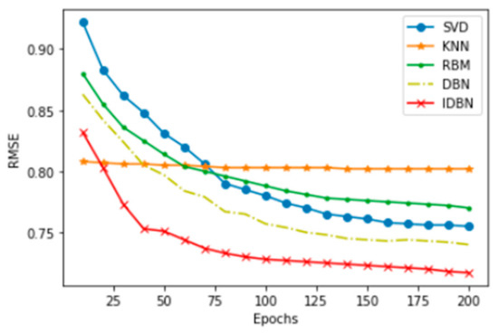
Figure 10.
The accuracy of the recommendation algorithm.
5. Conclusions and Future Work
This paper uses the basic idea of knowledge transfer to solve the problem that traditional DBN is difficult to quickly determine the best network structure. Through independent construction of the network structure, the traditional DBN structure is built into a larger complex network, so that DBN can obtain richer data characteristics and deeper abstract expression, and use the PLSR algorithm to fine-tune the network parameters of the self-constructed DBN. The PLSR algorithm avoids the gradient dispersion problem of the BP algorithm and greatly improves the fine-tuning accuracy. Finally, the IDBN structure with the best performance is obtained. In order to verify the prediction performance of the model, this paper conducts two types of prediction experiments on the public data sets of LFM-1k and ML-20M: popularity prediction based on time series and rating classification prediction based on user data. Compared with classic time series algorithms and traditional recommendation algorithms, IDBN is superior to other fixed models in terms of prediction performance and training time. However, in the training process, the DBN model also has limitations. Since the network connection weight parameters after self-construction are more, the representation vector of the input data cannot be too dense. Therefore, in the future work, the relationship between the sparse representation of the network and the performance of the model will be further studied to improve the efficiency of the algorithm. At the same time, the model should be run on a noisy industrial data set to improve the robustness of the model.
Author Contributions
Conceptualization, Y.Z. and F.L.; funding acquisition, F.L.; methodology, Y.Z.; software, Y.Z.; validation, Y.Z.; writing—original draft, Y.Z.; writing—review and editing, Y.Z. All authors have read and agreed to the published version of the manuscript.
Funding
This work was supported by the following grants: National Natural Science Foundation of China 61772321.
Conflicts of Interest
The authors declare no conflict of interest.
References
- Schmidhuber, J. Deep learning in neural networks: An overview. Neural Netw. 2015, 61, 85–117. [Google Scholar] [CrossRef] [PubMed]
- Valter, P.; Lindgren, P.; Prasad, R. The consequences of artificial intelligence and deep learning in a world of persuasive business models. IEEE Aerosp. Electron. Syst. Mag. 2018, 33, 80–88. [Google Scholar] [CrossRef]
- LeCun, Y.; Bengio, Y.; Hinton, G. Deep learning. Nature 2015, 521, 436. [Google Scholar] [CrossRef] [PubMed]
- Krizhevsky, A.; Sutskever, I.; Hinton, G.E. Imagenet classification with deep convolutional neural networks. In Advances in Neural Information Processing Systems; MIT Press: Cambridge, MA, USA, 2012; pp. 1097–1105. [Google Scholar]
- Mikolov, T.; Karafiát, M.; Burget, L. Recurrent neural network based language model. In Proceedings of the Eleventh Annual Conference of the International Speech Communication Association, Makuhari, Japan, 26–30 September 2010. [Google Scholar]
- Hinton, G.E.; Salakhutdinov, R. Reducing the dimensionality of data with neural networks. Science 2006, 313, 504–507. [Google Scholar] [CrossRef] [PubMed]
- Hinton, G.E.; Osindero, S.; Teh, Y.W. A fast learning algorithm for deep belief nets. Neural Comput. 2006, 18, 1527–1554. [Google Scholar] [CrossRef] [PubMed]
- Khatami, A.; Khosravi, A.; Nguyen, T.; Lim, C.P.; Nahavandi, S. Medical image analysis using wavelet transform and deep belief networks. Expert Syst. Appl. 2017, 86, 190–198. [Google Scholar] [CrossRef]
- De la Rosa, E.; Yu, W. Randomized algorithms for nonlinear system identification with deep learning modification. Inf. Sci. 2016, 364, 197–212. [Google Scholar] [CrossRef]
- Shen, F.; Chao, J.; Zhao, J. Forecasting exchange rate using deep belief networks and conjugate gradient method. Neurocomputing 2015, 167, 243–253. [Google Scholar] [CrossRef]
- Chen, T.; Goodfellow, I.; Shlens, I. Net2Net: Accelerating learning via knowledge transfer. arXiv 2015, arXiv:1511.05641. [Google Scholar]
- Lopes, N.; Ribeiro, B. Towards adaptive learning with improved convergence of deep belief networks on graphics processing units. Pattern Recognit. 2014, 47, 114–127. [Google Scholar] [CrossRef]
- Roy, P.P.; Chherawala, Y.; Cheriet, M. Deep-belief-network based rescoring approach for handwritten word recognition. In Proceedings of the 14th International Conference on Frontiers in Handwriting Recognition, Crete, Greece, 1–4 September 2014; pp. 506–511. [Google Scholar]
- Geng, Z.Q.; Zang, Y.K. An improved deep belief network inspired by Glia Chains. Acta Autom. Sin. 2016, 43, 943–952. [Google Scholar]
- Palomo, E.J.; López-Rubio, E. The growing hierarchical neural gas self-organizing neural network. IEEE Trans. Neural Netw. Learn. Syst. 2017, 28, 2000–2009. [Google Scholar] [CrossRef] [PubMed]
- Wang, G.M.; Qiao, J.F.; Bi, J. TL-GDBN: Growing deep belief network with transfer learning. IEEE Trans. Autom. Sci. Eng. 2018, 16, 874–885. [Google Scholar] [CrossRef]
- Afridi, M.J.; Ross, A.; Shapiro, E.M. On automated source selection for transfer learning in convolutional neural networks. Pattern Recognit. 2018, 73, 65–75. [Google Scholar] [CrossRef] [PubMed]
- Qiao, J.; Wang, G.; Li, W.; Li, X. A deep belief network with PLSR for nonlinear system modeling. Neural Netw. 2018, 104, 68–79. [Google Scholar] [CrossRef] [PubMed]
- He, Y.L.; Geng, Z.Q.; Xu, Y. A robust hybrid model integrating enhanced inputs based extreme learning machine with PLSR (PLSR-EIELM) and its application to intelligent measurement. ISA Trans. 2015, 58, 533–542. [Google Scholar] [CrossRef] [PubMed]
- Harper, F.M. The movielens datasets: History and context. ACM Trans. Int. Intell. Syst. 2015, 5, 1–19. [Google Scholar] [CrossRef]
- Li, F.; Qiao, J.; Han, H. A self-organizing cascade neural network with random weights for nonlinear system modeling. Appl. Soft Comput. 2016, 42, 184–193. [Google Scholar] [CrossRef]
- López-Yáñez, I.L.; Yáñez-Márquez, Y.C. A novel associative model for time series data mining. Pattern Recognit. Lett. 2014, 41, 23–33. [Google Scholar] [CrossRef]
- Ma, H.; King, I.; Lyu, M.R. Effective missing data prediction for collaborative filtering. In Proceedings of the 30th Annual International ACM SIGIR Conference on Research and Development in Information Retrieval, Amsterdam, The Netherlands, 23–27 July 2007; p. 46. [Google Scholar]
- Wang, J.; De Vries, A.P.; Reinders, M.J.T. Unifying user-based and item-based collaborative filtering approaches by similarity fusion. In Proceedings of the 29th Annual International ACM SIGIR Conference on Research and Development in Information Retrieval, Washington, DC, USA, 6–11 August 2006; p. 508. [Google Scholar]
Publisher’s Note: MDPI stays neutral with regard to jurisdictional claims in published maps and institutional affiliations. |
© 2020 by the authors. Licensee MDPI, Basel, Switzerland. This article is an open access article distributed under the terms and conditions of the Creative Commons Attribution (CC BY) license (http://creativecommons.org/licenses/by/4.0/).