Sustainable Communication Systems: A Graph-Labeling Approach for Cellular Frequency Allocation in Densely-Populated Areas


1
Department of Computer Science, Faculty of Science, Adekunle Ajasin University, Akungba 234034, Nigeria
2
Department of Geology, Faculty of Geography and Geoscience, University of Trier, Universitätsring 15, 54296 Trier, Germany
3
Center for Basic and Applied Research, Faculty of Informatics and Management, University of Hradec Kralove, Rokitanskeho 62, Hradec Kralove 50003, Czech Republic
*
Author to whom correspondence should be addressed.
Future Internet 2019, 11(9), 186; https://doi.org/10.3390/fi11090186
Submission received: 5 July 2019
/
Revised: 18 August 2019
/
Accepted: 20 August 2019
/
Published: 26 August 2019
(This article belongs to the Special Issue Smart Solutions in Development of Smart Applications and Systems with Aspect of Usefullness and Sustainability)
Abstract
:The need for smart and sustainable communication systems has led to the development of mobile communication networks. In turn, the vast functionalities of the global system of mobile communication (GSM) have resulted in a growing number of subscribers. As the number of users increases, the need for efficient and effective planning of the “limited” frequency spectrum of the GSM is inevitable, particularly in densely-populated areas. As such, there are ongoing discussions about frequency (channel) allocation methods to resolve the challenges of channel allocation, which is a complete NP (Nondeterministic Polynomial time) problem. In this paper, we propose an algorithm for channel allocation which takes into account soft constraints (co-channel interference and adjacent channel interference). By using the Manhattan distance concept, this study shows that the formulation of the algorithm is correct and in line with results in the literature. Hence, the Manhattan distance concept may be useful in other scheduling and optimization problems. Furthermore, this unique concept makes it possible to develop a more sustainable telecommunication system with ease of connectivity among users, even when several subscribers are on a common frequency.
1. Introduction
Due to its vast functions, the global system of the mobile communication (GSM) cellular network has experienced a rapid increase in the number of subscribers. As the number of users increases, the need for efficient and effective planning of the GSM’s “limited” frequency spectrum is inevitable, particularly in densely populated areas. As such, there are ongoing discussions regarding frequency (channel) allocation methods to resolve the challenges of channel allocation, which presents itself as an NP complete problem. Discourse on channel allocation has gained momentum in recent years, so that demand for a ratio spectrum (which is and will always remain a scarce commodity) has intensified [1,2,3]. Although the world has adopted faster communication technology, such as the 5G network, the structure of the GSM is the foundation upon which most new network structures are built, especially for voice and text messaging services [4,5]. While several advanced radio technologies are now popular, cellular network providers in some developing countries still adopt the Manhattan distance technique for GSM. The main reason for this is the high cost of new technologies such as 4G and 5G, which are yet be fully adopted. Nevertheless, since the range of cellular communication is of the utmost importance, newer methods have been developed to further increase the range of cellular networks. It is believed that the greater the level of optimization, the better it is for network communication and development in terms of cell-by-cell connectivity. In a study [6], a geometrical technique for determining cell range was developed. The technique utilizes a so-called Voronoi tessellation. The specific inputs needed for this technique include the location of the site, the beam width of the horizontal antennae, and the antenna azimuths. While this method has been shown to improve on the conventional technique, this improvement is still largely technically tied to the GSM basics.
In GSM technology, the allocation or assignment of planning frequency is crucial in the modern telecommunication regime. This is useful not only at the system commencement phase, but also at later stages of network modification or expansion, which should cater for high levels of interference and mass usage, among other factors [4,5,6]. Three channel allocation schemes have been identified in the literature [7,8], namely dynamic, fixed, and hybrid. Nevertheless, assigning a frequency remains a challenge [9]. Assume the existence of a set of channels which aids frequency transmission to a group of transmitters. In the vicinity of a dual transmitter, individual transmitters must use a different channel so as to maintain the needed transmission quality. The lowest uniqueness in frequencies assigned to dual transmitters in proximity is a function of their level of interference. The goal of frequency assignment is to locate the best possible assignment (given a frequency that is quite small) without compromising the quality of communication. The channel allocation problem is a class issue which is NP complete, implying that no existing algorithms (polynomial time) can solve this problem [10,11,12,13]
Definition 1: A graph is termed complete if it is simply constructed and undirected and has a unique pair of vertices linked by a different edge. In this study, Cn denotes a hypothetical scenario of a complete graph with n vertices, where a, b ∈ T, and (a, b) ∈ H represent the vertices [14].
Definition 2: Let U denote a graph that is undirected, let T represent a group of nodes, let E represent a group of lines connecting the nodes, and let C represent a group of colors. The process of mapping CT so that no corresponding vertices within the undirected graph, U, are allotted the same channel is referred to as “graph coloring”.
Definition 3: A cellular type grid denoted by Z and having a size r × c, where c and r are greater than or equal to 2, is derived from a bi-dimensional grid, A, which has a similar size. This is done by augmenting the group of edges using diagonal connections that extend from left to right. Specifically, each of the vertices of Z, represented by a = (n, m), is linked to another vertex, represented by b = (n − 1, m − 1) and d = (n + 1, m + 1). As a result, the vertex now possesses a degree of 6, excluding the vertices at the border regions.
Definition 4: A coloring algorithm, L(h,k), labels integers that are greater than 0 to the vertex U in a manner that allows neighboring nodes to be color-labeled and to be separated by at least a distance h; the same applies to the vertices (distance 2), which are also color-labeled and separated by at least a distance k. This coloring algorithm reduces the differences between the most and the least used colors, i.e., the span σh, k(U). The smallest span in other labeling functions is represented by λ h, k(U).
The rest of this paper is organized as follows. An overview of relevant literature regarding the resolution of channel allocation problems is presented in Section 2. Section 3 describes the methodology. Section 4 describes the experimental and evaluation procedures. Section 5 and Section 6 give conclusions and discuss possible future research on the subject, respectively.
2. Related Works
Recently, interest in algorithms which allow optimal channel allocation in cellular networks has soared. Some such algorithms focus on minimizing the span of the channel used, while others focus on minimizing interference [8,15]. In References [9,12,13,16] the authors studied cellular systems using algorithms to allocate channels. According to [17], channel allocation methods include fixed, dynamic, and hybrid types. Different approaches for channel allocation were discussed in [18], such as a central approach, a distributed approach, a relaxed mutual approach, and a genetic algorithm approach. In [17,18], a genetic algorithm was used to study channel allocation in wireless communication systems and to try and develop solutions to challenges arising from channel assignment [19,20]. As a result, two strategies were developed: in the first “Genetic Algorithm Lock” (GAL), already assigned channels are locked when a call is on hold [21]; in the second “Genetic Algorithm Switch” (GAS), there is the possibility of switching a call to another channel during a connection phase [22]. Both of these studies noted the need to allocate the correct channel, as well as the challenges associated with assigning channels (especially in cellular networks) to new geographical settings so as to reduce the entire span of frequency, which is a function of demand and interference-free constraints, referred to as “Channel Assignment Problem 1” (CAP1), or to reduce interference, which depends on demand constraints, called “Channel Assignment Problem 2” (CAP2). However, it was observed in [23] that the used method, Genetic Algorithm (GA), was unable to reduce the reuse frequency, even though channel allocation was carried out. By studying common allocation systems in mobile networks [24], reference [25] developed a unique centralized channel allocation which could effectively use scarce resource bandwidth. This model contains the so-called geographical model, which is essentially a group of contiguous, non-overlapping cells, each of which has a hexagonal form and which together form a parallelogram. The same study proposed a traffic model which mainly involves a dynamic channel allocation system in which there are no fixed channels. Hence, as soon as a call arrives, it is seen as a random process, and the function N (t) for all t ≥ 0 and the interval (0, t) is used to decode the number of arriving calls. The procedure for determining the number of arriving calls N (t), t*0 is a Poisson procedure that has an average rate λ. A modern algorithm technique, namely the “Particle Swarm Optimization” [26,27,28,29], was adopted for channel allocation [30]. This technique depends on a worldwide optimization that depends on “bird flocking” social behavior. It has the features of both swarm-based and agent-based techniques, making it a rapid process, and its characteristics are different to those of common evolutionary algorithms (EA) such as those presented in [31]. The evolutionary algorithms mainly deal with channel allocation, and do not allow the minimization of frequency reuse distance.
2.1. The L(2,1) Algorithm
Definition 5: Let U be a graph that is undirected and has a group of nodes, T, connected by some groups of lines, E. Let the function f:T ≥ N, where f refers to the L(2,1) graph labeling of the undirected graph. If for all a, b € T, |f(a) − f(b)| ≥ 2 if d(a, b) = 1 and |f(a) − f(b)| ≥ 1 if d(a, b) = 2 [32,33].
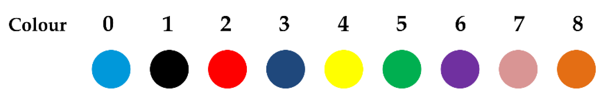
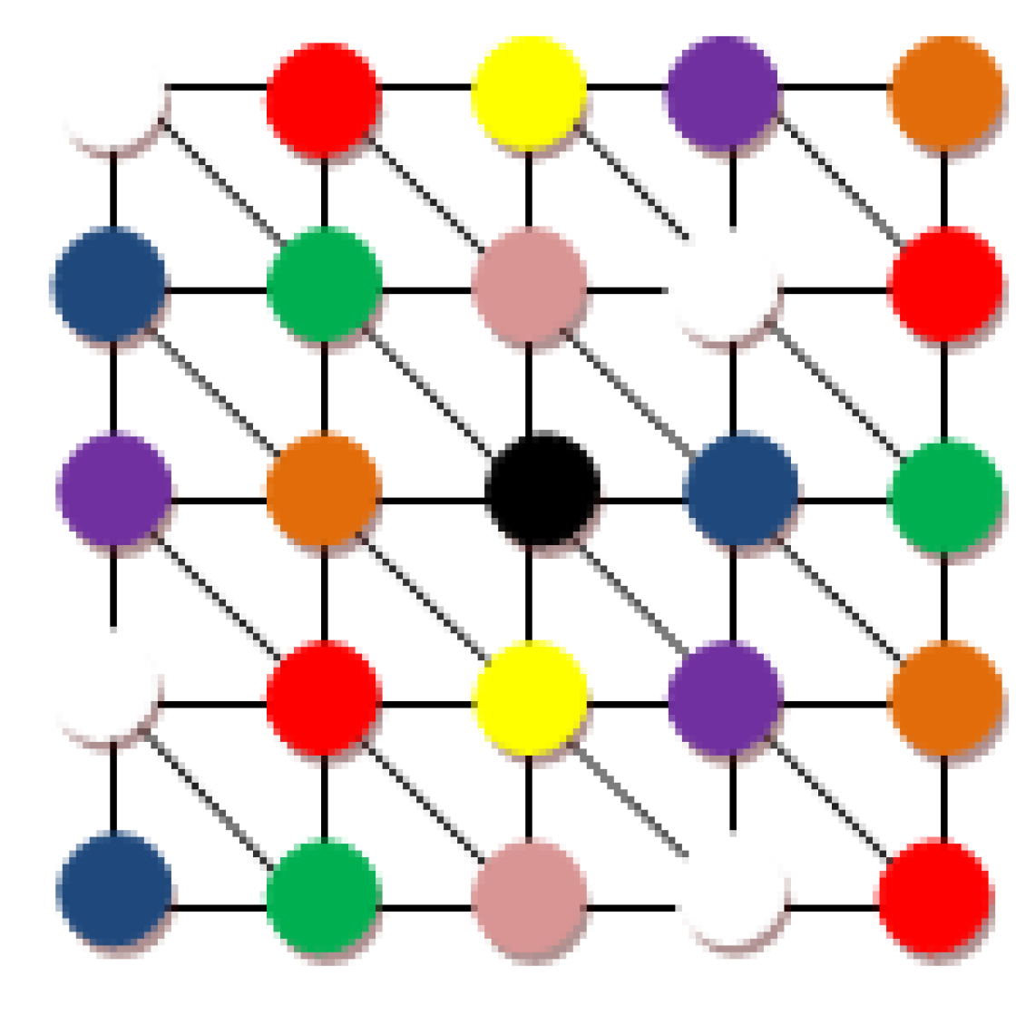
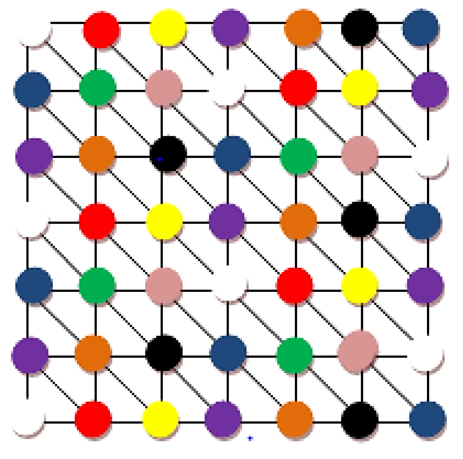
Several researchers have studied the L(2,1) coloring under different names, such as radio coloring, or coloring. Reference [8] proved N-completeness in graph coloring using the L(2,1) graph condition. According to [34], coloring a graph with this algorithm depends on the group of vertices T(G) and the group of all non-negative integers such that |f(a) – f(b)| ≥ 1 if d(a, b) = 2 and |f(a) – f(b)| ≥ 2 if d(a, b) = 1 [35,36]. The clique and algorithm for the L(2,1) coloring was proposed by [2] for a cellular network with n rows and m columns. Nine colors were used to color the L(2,1) clique. For this labeling, if n ≥ 4 and m ≥ 4, or n ≥ 3 and m ≥ 5 or n ≥ 5 and m ≥ 3, color a node x = (n, m) with color f(a) = (3n + 2m) % 9, where x is a vertex with n and m rows and columns, respectively. Figure 1 shows the numbers of colors used for the L(2,1) coloring, while Figure 2 and Figure 3 show some matrices colored with the L(2,1) coloring.
2.2. The L(2,1,1) Algorithm
Definition 6: Let U be a graph which is undirected and has a group of vertices T and a group of edges E. Let the function f:T ≥ N, where f is a L(2,1,1) labeling of U, if for all a, b € T, |f(a) − f(b)| ≥ 2 if d(a, b) = 1, |f(a) − f(b)| ≥ 1 if d(a, b) = 2 and the distance between colors assigned to a, b differs by at least two units in the color spectrum [7,11].
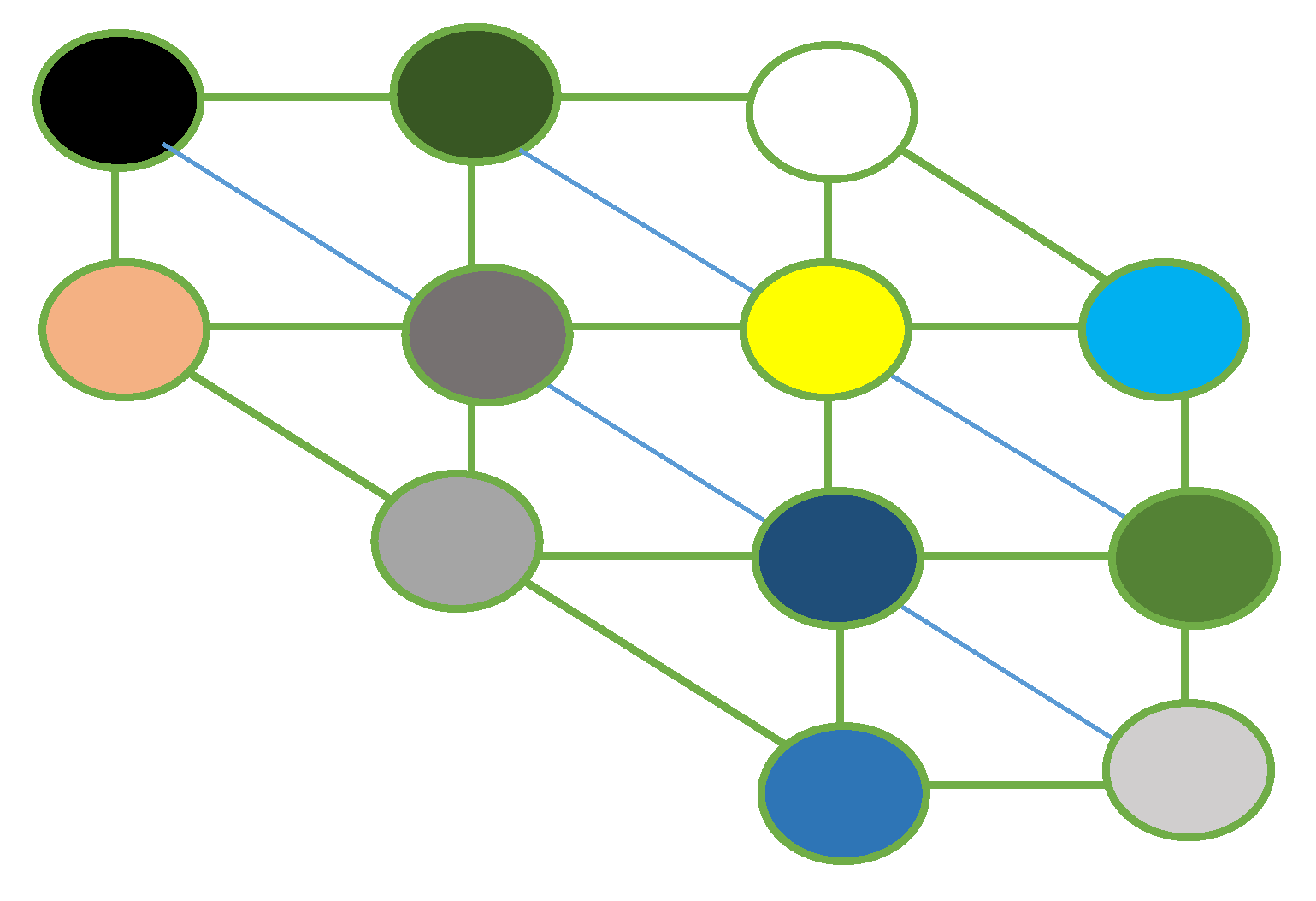
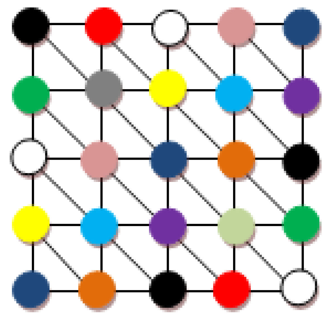
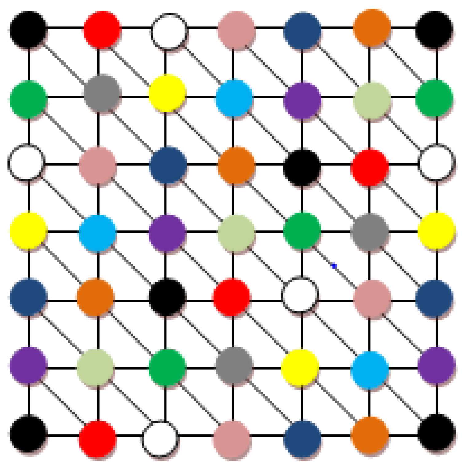
Figure 4 shows the colors used for the labeling, while Figure 5 shows the clique of the labeling. The reuse distance for this labeling is four (i.e., ϕ = 4). According to [16], a graph’s coloring problem, which is the problem of assigning colors to certain nodes of a graph based on some constraints, can be solved by using a clique; this clique is subsequently colored using an algorithm that is suitable for this purpose. The same method of clique coloring can be adopted in a matrix of any size in a cellular graph. Figure 6 shows the L(2,1,1) labeling of a 5 × 5 network graph, while Figure 7 shows a 7 × 7 network graph colored using the L(2,1,1) coloring. In formulation, the parities of i and j are considered, with the modulus (represented by %) being used in the formulation to achieve the optimal coloring of the clique.
For the L(2,1,1) graph coloring, [16] proposed the following algorithm: for n rows and m columns, if n ≥ 4 and m ≥ 4, then the color f(a) is assigned to a node G = (i, j) thus:
0 if (i + j) = 2 % 6, n is even, and m is even; 1 if (i + j) = 0 % 6, n is even, and m is even;
2 if (i + j) = 4 % 6, n is even, and m is even; 3 if (i + j) = 1 % 6, n is odd, and m is even;
4 if (i + j) = 3 % 6, n is odd, and m is even; 5 if (i + j) = 5 % 6, n is odd, and m is even;
6 if (i + j) = 5 % 6, n is even, and m is odd; 7 if (i + j) = 2 % 6, n is odd, and m is odd;
8 if (i + j) = 4 % 6, n is odd, and m is odd; 9 if (i + j) = 1 % 6, n is even, and m is odd;
10 if (i + j) = 3 % 6, n is even, and m is odd; 11 if (i + j) = 0 % 6, n is odd, and m is odd.
3. Method
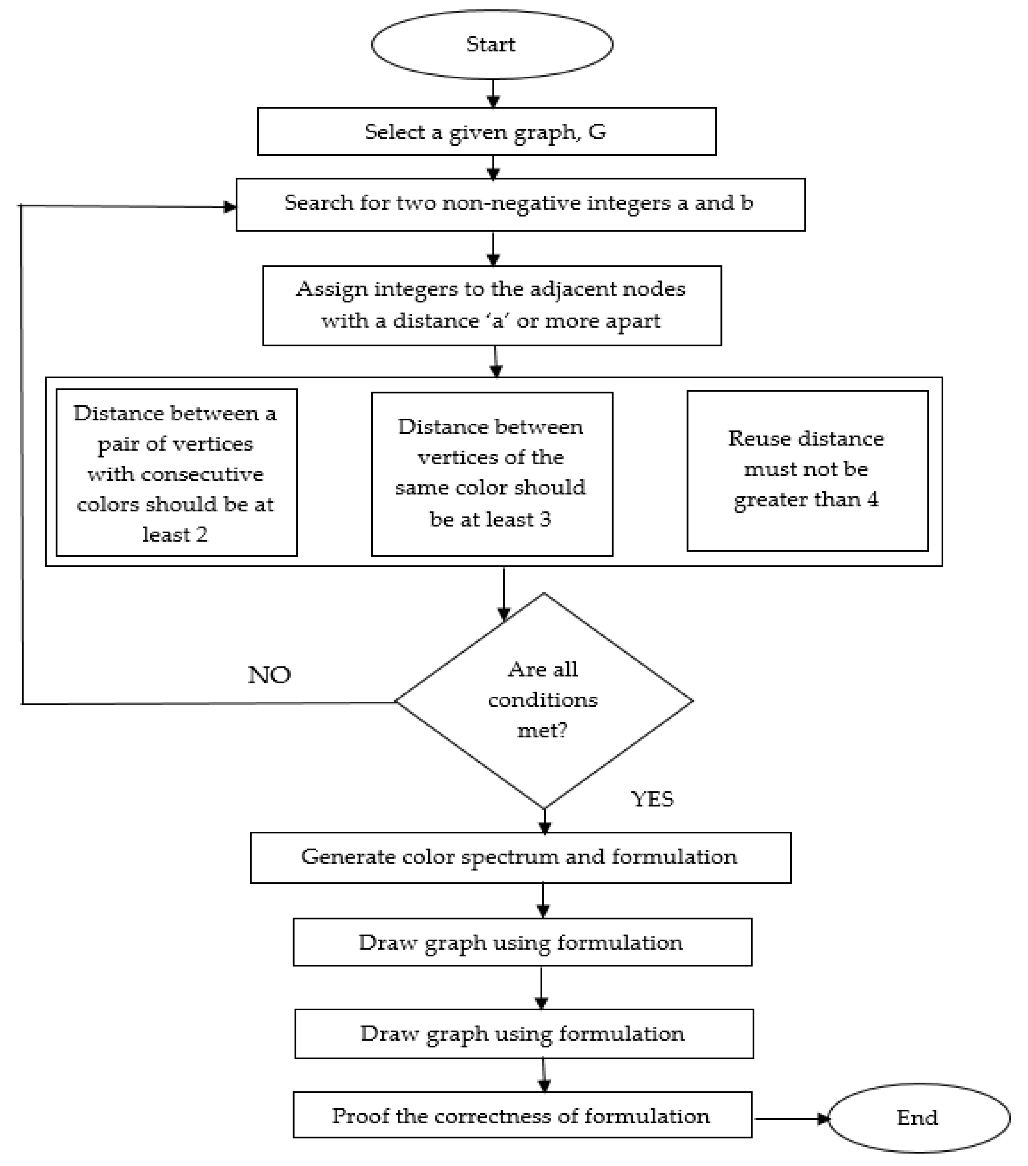
Definition 7: Let U represent a graph which is not directed and has a group of vertices and edges represented by T and E, respectively. Let the function f:T ≥ N, where f is a L(3,1) labeling of U, if for all a, b € T, |f(a) − f(b)| ≥ 3 if d(a, b) = 1 and |f(a) − f(b)| ≥ 1 if d(a, b) = 3. For this labeling, a pair of vertices with a pair of consecutive colors should be separated by a minimum of one unit, while vertices with the same color must be separated by at least three units. Figure 8 shows the flowchart for the formulation of the L(3,1) algorithm.
Proposition 1: To color the graph U = (T, E) (which is undirected), we use L(3,1), λ = 12.
Proof: Given the cellular grid Z = (T, E) from definition 3, we obtain two different graphs: a subgraph D of Z, as shown in Figure 9, and an augmented graph UC,4 = (T, E’). A clique is developed in UC,4 by all of the vertices from Z, with each vertex assigned a unique color; hence, λ(Z) = 12. Hence, for all r, if a cellular grid exists with n rows and m columns, if n ≥ 7 and m ≥ 9, then the L(3,1) coloring has the function f(a) = ((7n + 9m) % 12)k □.
Hence, the formulation of the L(3,1) algorithm is: if n ≥ 7 and m ≥ 9, then the following colors representing f(a) can be assigned to each vertex U = (n, m):
0 if (7n + 9m) % 12 ≡ 0 % 12 and both i and j are even; 9 if (7n + 9m) % 12 ≡ 9 % 12, i is even, and j is odd; 6 if (7n + 9m) % 12 ≡ 6 % 12 and both i and j are even; 3 if (7n + 9m) % 12 ≡ 3 % 12 and both i and j are even; 7 if (7n + 9m) % 12 ≡ 7 % 12 and both i and j are even; 4 if (7n + 9m) % 12 ≡ 4 % 12 and both i and j are odd; 1 if (7n + 9m) % 12 ≡ 1 % 12, i is odd, and j is even; 10 if (7n + 9m) % 12 ≡ 10 % 12 and both i and j are odd; 2 if (7n + 9m) % 12 ≡ 2 % 12 and both i and j are even; 11 if (7n + 9m) % 12 ≡ 11 % 12, i is even, and j is odd; 8 if (7n + 9m) % 12 ≡ 8 % 12 and both i and j are even; and 5 if (7n + 9m) % 12 ≡ 5 % 12, i is even, and j is odd.
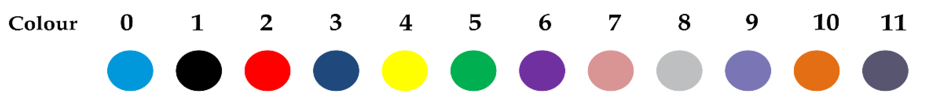
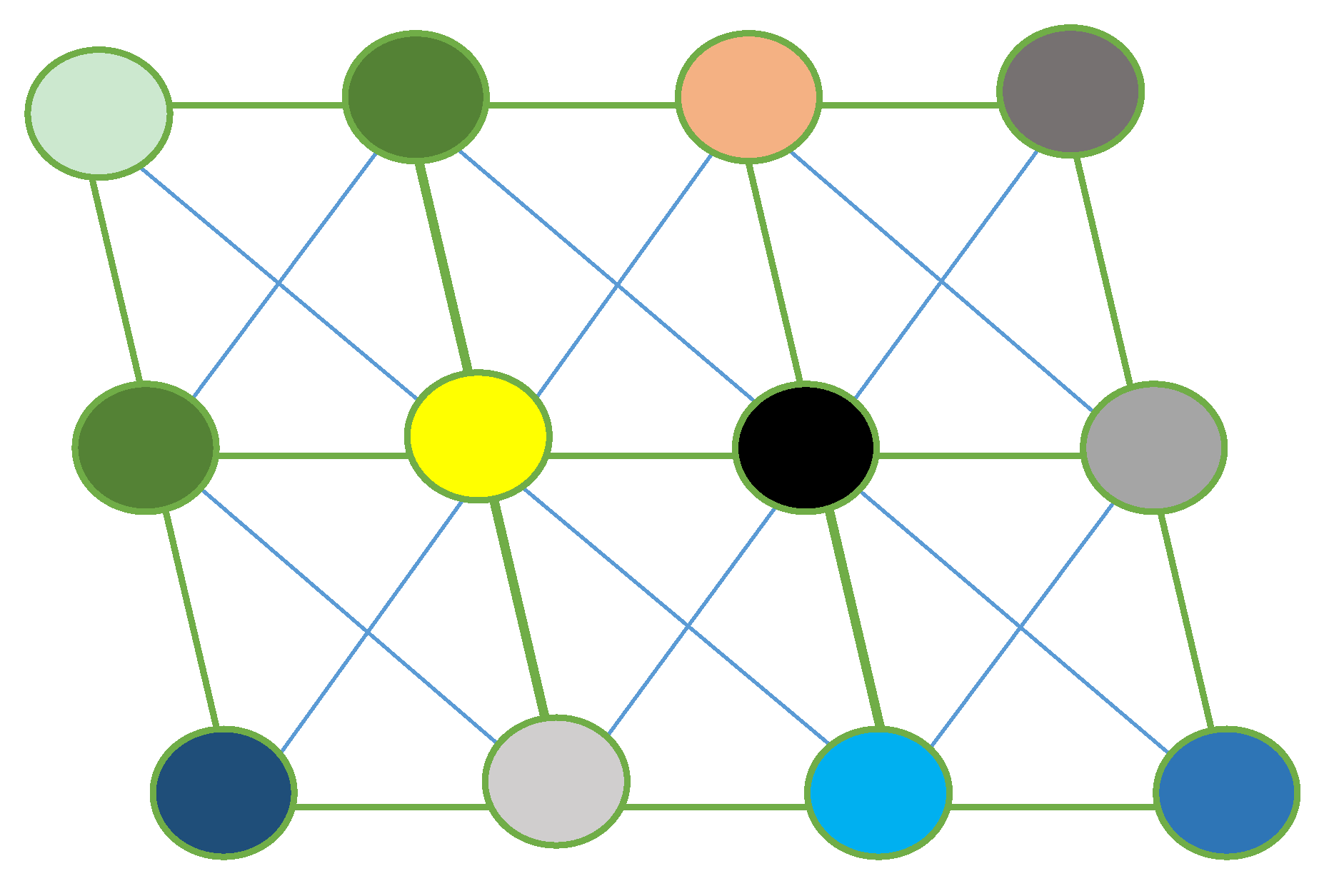
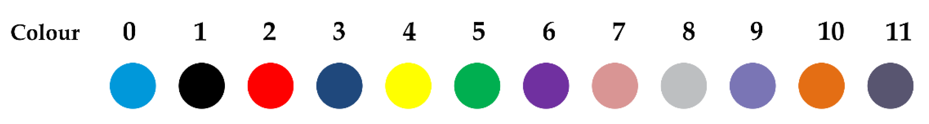
The vertex numbering (for a 10 × 10 matrix) and color spectrum for the L(3,1) algorithm are shown in Table 1. Using the formulation for L(3,1) generated in the previous section, m × n matrix grids are colored using the color spectrum shown in Figure 10. A 5 × 5 network graph colored using the L(3,1) labeling is presented in Figure 11, while Figure 12 shows a 10 × 10 network graph colored using the L(3,1) labeling.
4. Results and Discussion
4.1. Checking the Correctness of the L(3,1) Coloring Algorithm
To prove the correctness of the coloring algorithms, we adopted the Manhattan distance concept [33]. To prove that successive colors have a spacing equal to 2, an assessment of the smallest distance separating consecutive colors was performed. Table 2 shows the parities of i and j.
As shown in Table 2, each pair of consecutive colors [(0,1), (1,2), (2,3), (3,4), (4,5), (5,6), (6,7), (7,8), (8,9), (9,10) and (10,11)] has a Manhattan distance of at least 3. According to Table 1, the lowest spacing between colors should be at least 2. Other sets of successive color pairs, such as (0,1), (3,4), (4,5), (7,8), and (9,10), have a Manhattan distance of at least 2 and have a similar parity for the n and m coordinates of both of their component colors. Note that in Figure 14, any random vertex (n, m) and another vertex (n’, m’) have a Manhattan distance of 2. The separation between them will not be less than 1, except when n and n’, or m and m’, have unique parities. Hence, these two vertices are separated by a minimum of 2 coloring units. It can thus be deduced that the distance between two vertices possessing the same color is ≥3. From the function of a vertex (a) of the L(3,1) algorithm, it is possible to infer that vertices with similar colors also possess similar parities for coordinates i or j. As shown in Table 2, none of the parity pairs (i and j coordinates) for the consecutive color pairs are the same. Therefore, from these observations, it can be seen that the vertices with the same color are separated by a distance of more than three units. This implies that the second definition holds true. Hence, the f(a) coloring of L(3,1) holds true for a given cellular graph matrix. Additionally, it can be observed from Figure 14 that the distance between two vertices of the same color is at least four units. Thus, the reuse distance is four (i.e., σ = 4), which satisfies the third condition for correctness. This evaluation of the Manhattan distance and the minimum distance between pairs of consecutive colors therefore proves the correctness of the L(3,1) algorithm.
4.2. Design of Channel Group Allocation
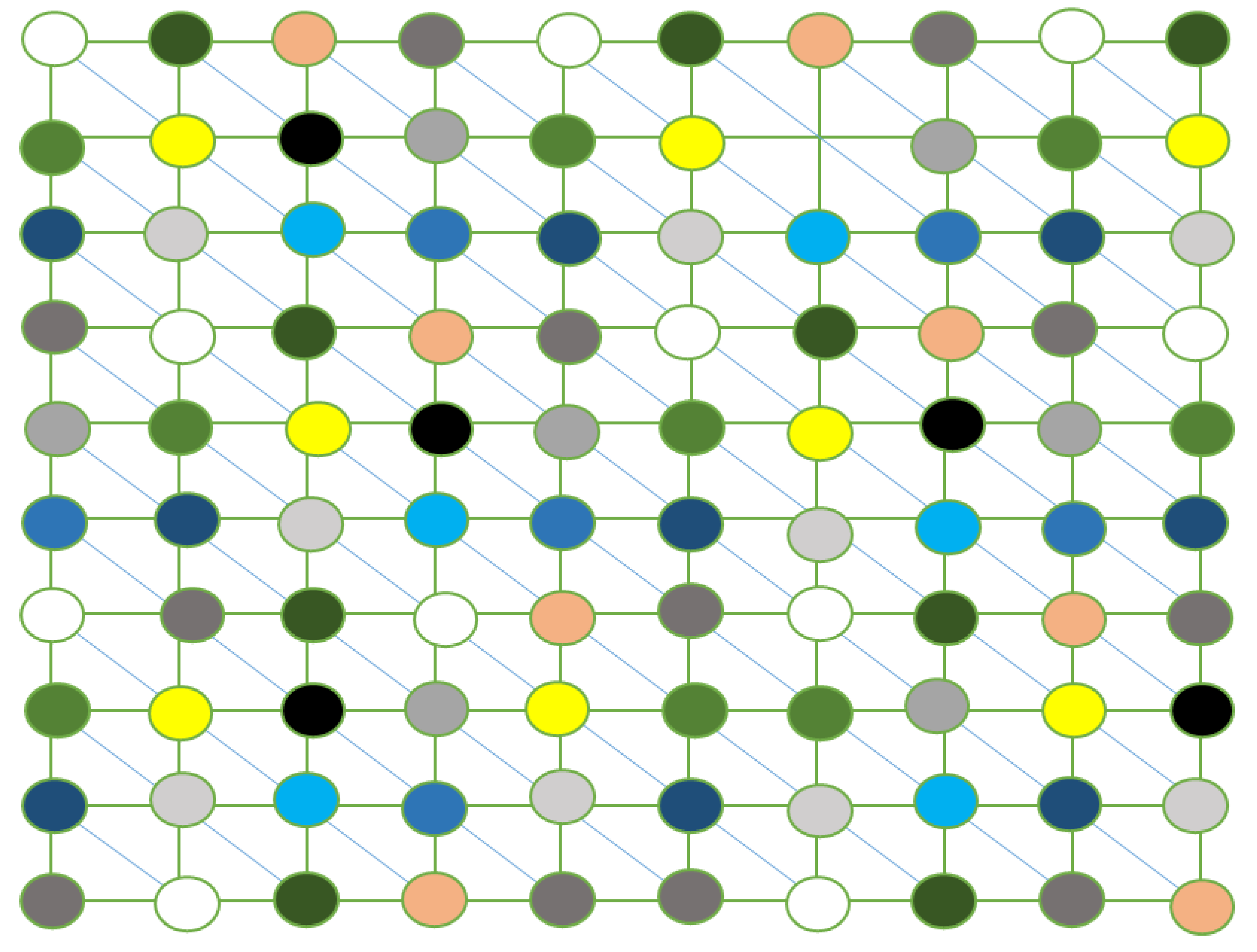
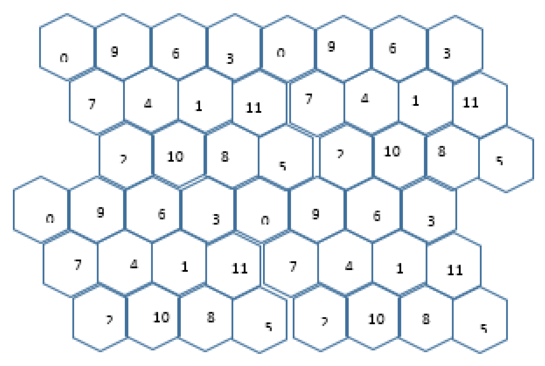
Figure 13 shows a hypothetical design procedure for channel allocation sets to cellular base stations, where there are 12 channels in a cell cluster (i.e., N = 12).
Considering a circular section of the cluster segment from Figure 14, the reuse distance can be calculated for the grid cells. The center spread between two co-channel cells is known as the reuse distance. The cluster size in the grid as shown in Figure 14 is equal to 12.
Co-channel reuse means that within a specific area of coverage there are many cells utilizing a similar group of channels [37]. Such cells are called co-channel cells. Co-channel cells also exhibit interference signals, which are referred to as co-channel interference. The only way to eliminate co-channel interference is by ensuring that the cells are separated by a sufficient distance [38]. In [39], the authors showed that in situations where cell sizes and base station power transmission are equal, the ratio of co-channel interference is often not a function of the power transmitted, but rather, that it depends on the cell radius (R) and the center spread of the nearest co-channel cells (D).
4.3. Method for Calculating the Reuse Distance
The method for calculating the distance ‘D’ from the center of one co-channel cell to the other is as explained as follows; given that A and B are co-channel cells, is the angle from one co-channel to the other. Therefore,
The co-channel reuse ratio is given as
Thus, for the L(3,1) coloring algorithm of the hypothetical cellular grid shown in Figure 14, the co-channel reuse ratio is
where N is the cluster size and is equal to 12. Thus,
Q is related to cluster size. In a six-sided geometry,
Q=D/R = √ (3N).
A small value of Q indicates a bigger capacity of the network grid due to the small cluster magnitude. Meanwhile, a large value of Q implies a higher transmission quality as a result of reduced co-channel interference. Thus, the cellular grid in Figure 14 labeled with the L(3,1) algorithm improves signal transmission quality and reduces co-channel interference.
4.4. Time Complexity for Selected Algorithms
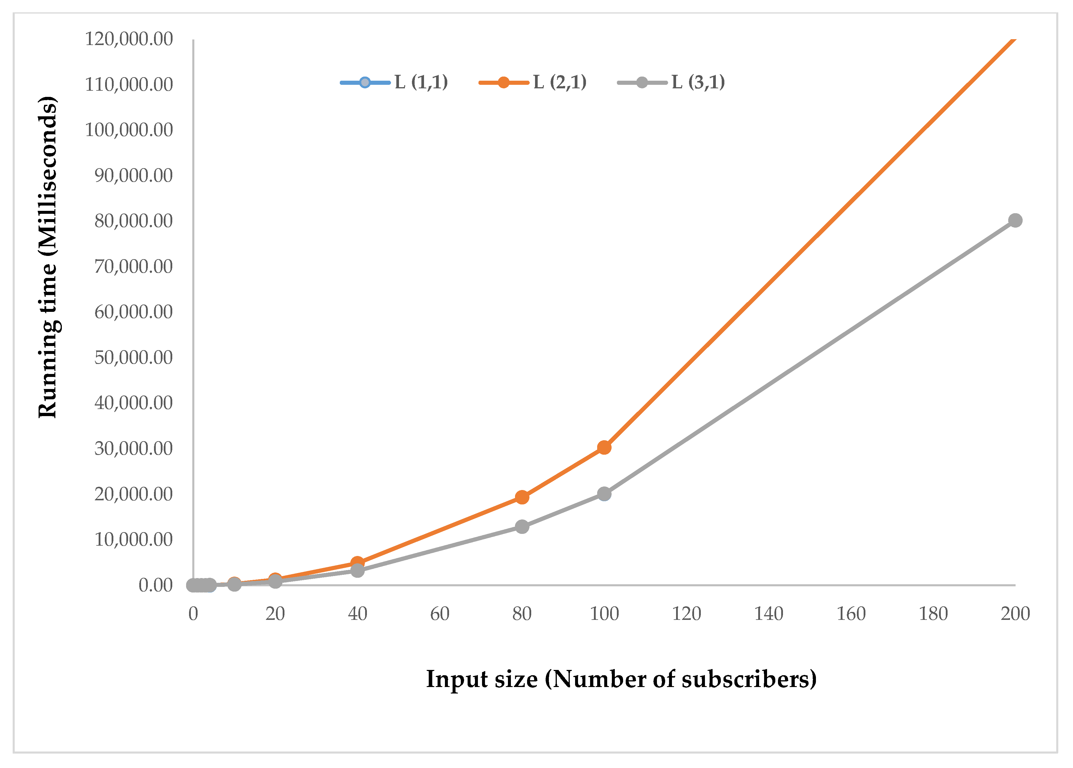
The “Big O” notation was used to check the complexity of each of the L(h,k) algorithms studied, with h = 1,2,3 and k = 1, for different input sizes. Table 3 indicates the running times of the algorithms for different input sizes.
Figure 15 shows a comparison of the running times of the three L(h,k) algorithms for different input sizes. The figure shows that, given a large amount of subscribers, the L(3,1) algorithm outperforms the L(2,1) algorithm (i.e., the L(3,1) algorithm has a smaller running time). This indicates that when there is a large number of users (e.g., in a densely populated area), the L(3,1) algorithm will perform optimally for channel allocation.
5. Conclusions
In an urban setting, network traffic demands are usually high, and network infrastructure operates at maximum or near-maximum capacity. In such a setting, traffic patterns may at first appear random and non-uniform. Such patterns are usually a function of time of day, population distribution, season, weather, special events (fans at a football stadium, conferences, festivals), etc. This study investigated various graph-coloring algorithms, and developed an improved and optimal L(3,1) graph-coloring algorithm to color a hexagonal cellular graph matrix (m × n). This algorithm was based on the Fixed Channel Allocation (FCA) scheme. Cell grids are permanently stationed and located at the same distance from the nodes. This study resolved the challenge posed by co-channel interference by creating a co-channel reuse distance, σ. Additionally, the problem caused by interference from adjacent channels was resolved by imposing channel separation. It was observed that channel gap has an inverse relationship with the distance between stations. Other constraints taken into account were interference between adjacent channels, as well as co-channel interference. These findings suggest appropriate changes that network providers can make to channel allocation to maximize channel assignments which bring about transmission efficiency.
6. Future Work
The challenges posed by frequency interference, among other issues in modern day telecommunication networks, raise questions about the sustainability of the global system of mobile communication (GSM). Several techniques have been proposed to resolve issues related to frequency interference, including the genetic algorithm and ordering heuristic. All of the existing methods which aim to solve the problem of network interference have shortcomings. As a result, this study proposes a new algorithm based on graph labeling. Sustainable communication networks bring socioeconomic improvement [40,41,42,43]. Removing interference improves communication flow. The novel graph-labeling technique for allocating frequency domains that is proposed in the present study can be used in future investigative works [44,45]. Future research should also endeavor to investigate the synchronization of graph coloring with other interference-reducing methods.
Author Contributions
Conceptualization, A.O., O.F., and O.K.; methodology, O.F., and O.K.; software, A.O. and O.F.; validation, O.F., and O.K.; formal analysis, O.F.; investigation, A.O.; resources, O.K., and O.F.; data curation, A.O., and O.F.; writing—original draft preparation, A.O. and O.F.; writing—review and editing, A.O., O.F., and O.K.; visualization, O.F., A.O.; supervision, O.F., and O.K.; project administration, O.F., and O.K.; funding acquisition, O.K.
Funding
The work and the contribution were supported by the SPEV project, University of Hradec Kralove, FIM, Czech Republic (ID: 2103–2019), “Smart Solutions in Ubiquitous Computing Environments”.
Acknowledgments
We are grateful for the support of student Sebastien Mambou and Michal Dobrovolny in consultations regarding application aspects. The APC was funded by the SPEV project, University of Hradec Kralove, FIM, Czech Republic (ID: 2012–2019), “Smart Solutions in Ubiquitous Computing Environments”.
Conflicts of Interest
The authors declare no conflict of interest.
References
- Kuboye, B.M.; Alese, B.K.; Fajuiyigbe, O.; Adewale, S.O. Development of Models for Managing Network Congestion on Global System for Mobile Communication (GSM) in Nigeria. J. Wirel. Netw. Commun. 2011, 1, 8–15. [Google Scholar]
- Haider, B.; Zafrullah, M.; Islam, M.K. Radio Frequency Optimization & QoS Evaluation in Operational GSM Network. In Proceedings of the world Congress on Engineering and Computer Science, San Francisco, CA, USA, 20–22 October 2009; pp. 1–6. [Google Scholar]
- Józefowicz, R.; Poźniak-Koszałka, I.; Koszałka, I.L.; Kasprzak, A. Algorithms for Solving Frequency Assignment Problem in Wireless Networks. In Recent Developments in Computational Collective Intelligence; Badica, A., Trawinski, B., Nguyen, N., Eds.; Springer: Cham, Switzerland, 2014; Volume 513, pp. 135–144. [Google Scholar]
- Biral, A.; Centenaro, M.; Zanella, A.; Vangelista, L.; Zorzi, M. The challenges of M2M massive access in wireless cellular networks. Digit. Commun. Netw. 2015, 1, 1–19. [Google Scholar] [CrossRef]
- Landström, S.; Bergström, J.; Westerberg, E.; Hammarwall, D. NB-IoT: A sustainable technology for connecting billions of devices. Ericsson Technol. Rev. 2016, 4, 2–11. [Google Scholar]
- Garcia, A.J.; Buenestado, V.; Toril, M.; Luna-Ramírez, S.; Ruiz, J.M. A Geometric Method for Estimating the Nominal Cell Range in Cellular Networks. Mob. Inf. Syst. 2018, 2018, 3479246. [Google Scholar]
- Mouly, M.; Pautet, M.B. The GSM System for Mobile Communications. Available online: https://dl.acm.org/citation.cfm?id=573838 (accessed on 21 August 2019).
- Hamad-Ameen, J.J. Frequency Planning in GSM Mobile. In Proceedings of the TELE-INFO’08 Proceedings of the 7th WSEAS International Conference on Telecommunications and Informatics, Istanbul, Turkey, 27–30 May 2008. [Google Scholar]
- Xu, Y.; Sakho, I. Frequencies Assignment in Cellular Networks. In Intelligent Information and Database Systems; Springer: Cham, Switzerland, 2015. [Google Scholar]
- Rughooputh, S.; Coomar, H.; Cheeneebash, J. A Comprehensive Review of Methods for the Channel Allocation Problem; African Minds: Cape Town, South Africa, 2014. [Google Scholar]
- Nurelmadina, N.; Nafea, I.; Younas, M. Evaluation of a channel assignment scheme in mobile network systems. Hum.Centric Comput Inf. Sci. 2016, 6, 1–15. [Google Scholar] [CrossRef]
- Idoumghar, L.; Debreux, P. New modeling approach to the frequency assignment problem in broadcasting. IEEE Trans. Broadcast. 2002, 48, 293–298. [Google Scholar] [CrossRef]
- Gozupek, D.; Genc, G.; Ersoy, C. Channel assignment problem in cellular networks: A reactive tabu search approach. In Proceedings of the 2009 24th International Symposium on Computer and Information Sciences, Guzelyurt, Cyprus, 23 October 2009. [Google Scholar]
- Katzela, I.; Naghshineh, M. Channel assignment schemes for cellular mobile telecommunication systems: A comprehensive survey. IEEE Commun. Surv. Tutor. 1996, 3, 10–31. [Google Scholar] [CrossRef]
- Peng, Y.; Wang, L.; Soong, B.H. Optimal channel assignment in cellular systems using tabu search. In Proceedings of the 14th IEEE Proceedings on Personal, Indoor and Mobile Radio Communications, Beijing, China, 7–10 September 2003. [Google Scholar]
- Bertossi, A.A.; Pinotti, C.M.; Tan, R.B. Efficient Use of Radio Spectrum in Wireless Networks with Channel Separation Between Close Stations. In Proceedings of the 4th International Workshop on Discrete Algorithms and Methods for Mobile Computing and Communication, Boston, MA, USA, 11 August 2000. [Google Scholar]
- Tech Republic, Hybrid Channel Allocation in Wireless Cellular Networks. Available online: https://www.techrepublic.com/resource-library/whitepapers/hybrid-channel-allocation-in-wireless-cellular-networks (accessed on 21 August 2019).
- Davis, J.S. Channel Allocation. Available online: http://www.wirelesscommunication.nl/reference/chaptr04/cellplan/dca.htm (accessed on 21 August 2019).
- Li, J.; Shroff, N.B.; Chong, E.K.P. A new localized channel sharing scheme for cellular networks. Wirel. Netw. 1999, 5, 503–517. [Google Scholar] [CrossRef]
- Kim, J.-S.; Park, S.; Dowd, P.; Nasrabadi, N. Channel assignment in cellular radio using genetic algorithms. Wirel. Pers. Commun. 1996, 3, 273–286. [Google Scholar] [CrossRef] [Green Version]
- Duran, M. How to Unlock Your Phone’s Trusty Call-Blocking Powers. Available online: https://www.wired.com/2016/07/unlock-phones-trusty-call-blocking-powers/ (accessed on 21 August 2019).
- Acampora, A.S. An Introduction to Broadband Networks: LANs, MANs, ATM, B-ISDN, and Optical Networks for Integrated Multimedia Telecommunications; Springer Science & Business Media: Berlin/Heidelberg, Germany, 2013. [Google Scholar]
- Ali, N.A.; El-Dakroury, M.A.; El-Soudani, M.; ElSayed, H.M.; Daoud, R.M.; Amer, H.H. New hybrid frequency reuse method for packet loss minimization in LTE network. J. Adv. Res. 2015, 6, 949–955. [Google Scholar] [CrossRef] [PubMed]
- Jiang, F.; Wang, H.; Ren, H.; Xu, S. Energy-efficient resource and power allocation for underlay multicast device-to-device transmission. Future Internet 2017, 9, 84. [Google Scholar] [CrossRef]
- Chu, Ta.; Rappaport, S.S. Generalized fixed channel assignment in microcellular communication systems. IEEE Trans. Veh. Technol. 1994, 43, 713–721. [Google Scholar]
- Idris, I.; Selamat, A.; Nguyen, N.T.; Omatu, S.; Krejcar, O.; Kuča, K.; Penhaker, M. A combined negative selection algorithm-particle swarm optimization for an email spam detection system. Eng. Appl. Artif. Intell. 2015, 39, 33–44. [Google Scholar] [CrossRef]
- Yin, L.; Li, X.; Lu, C.; Gao, L. Energy-efficient scheduling problem using an effective hybrid multi-objective evolutionary algorithm. Sustainability 2016, 8, 1268. [Google Scholar] [CrossRef]
- Salehi, S.; Selamat, A.; Krejcar, O.; Kuca, K. Fuzzy granular classifier approach for spam detection. J. Intell. Fuzzy Syst. 2017, 32, 1355–1363. [Google Scholar] [CrossRef]
- Lim, K.C.; Selamat, A.; Zabil, M.H.M.; Selamat, M.H.; Alias, R.A.; Puteh, F.; Mohamed, F.; Krejcar, O.; Herrera-Viedma, E.; Fujita, H. Feasibility comparison of HAC algorithm on usability performance and self-reported metric features for MAR learning. In Proceedings of the 17th International Conference on New Trends in Intelligent Software Methodology Tools and Techniques (SoMeT 2018), Granada, Spain, 26–28 September 2018; pp. 896–910. [Google Scholar]
- Zhang, Y.; Wang, S.; Ji, G. A Comprehensive Survey on Particle Swarm Optimization Algorithm and Its Applications. Math. Probl. Eng. 2015, 2015, 931256. [Google Scholar] [CrossRef]
- Bäck, T.; Hoffmeister, F. Extended Selection Mechanisms in Genetic Algorithms. In Proceedings of the Fourth International Conference on Genetic Algorithms, San Diego, CA, USA, 13–16 July 1991. [Google Scholar]
- Shao, Z. The Research on the L(2,1)-labeling problem from Graph theoretic and Graph Algorithmic Approaches. 2012. Available online: https://ir.lib.uwo.ca/cgi/viewcontent.cgi?article=1604&context=etd (accessed on 21 August 2019).
- Tsang, V.; Stevenson, S. A Graph-theoretic Framework for Semantic Distance. Comput. Linguist. 2010, 36, 31–69. [Google Scholar] [CrossRef]
- Klavzar, S.; Vesel, A. Computing graph invariants on rotagraphs using dynamic algorithm approach: the case of (2,1)-colorings and independence numbers. Discrete Appl. Math. 2003, 129, 449–460. [Google Scholar] [CrossRef] [Green Version]
- Matula, D.W.; Marble, G.; Isaacson, J.D. Graph Coloring Algorithm. In Graph Theory and Computing; Read, R.C., Ed.; Academic Press: Cambridge, MA, USA, 1972; pp. 109–122. [Google Scholar]
- Wigderson, A. A New Approximate Graph Coloring Algorithm. In Proceedings of the Fourteenth Annual ACM Symposium on Theory of Computing, San Francisco, CA, USA, 5–7 May 1982. [Google Scholar]
- Lee, W.C.Y. Chapter 46: Cellular Telecommunications Systems. In Reference Data for Engineers, 9th ed.; Middleton, W.M., Van Valkenburg, M.E., Eds.; Newnes: Woburn, MA, USA, 2002; p. 1. [Google Scholar]
- Adediran, Y.A.; Lasisi, H.; Okedere, O.B. Interference management techniques in cellular networks: A review. Cogent Eng. 2017, 4, 1294133. [Google Scholar] [CrossRef]
- Horalek, J.; Sobeslav, V.; Krejcar, O.; Balik, L. Communications and security aspects of smart grid networks design. In Proceedings of the International Conference on Information and Software Technologies; Springer: Cham, Switzerland, 2014; pp. 35–46. [Google Scholar]
- Klimova, B.; Maresova, P. Social network sites and their use in education. In Emerging Technologies for Education; Wu, T.T., Gennari, R., Huang, Y.M., Xie, H., Cao, Y., Eds.; Springer: Cham, Switzerland, 2017. [Google Scholar]
- Hruska, J.; Maresova, P. Design of business canvas model for social media. In Emerging Technologies in Data Mining and Information Security; Springer: Singapore, 2019. [Google Scholar]
- Deen, M.J. Information and communications technologies for elderly ubiquitous healthcare in a smart home. Pers. Ubiquitous Comput. 2015, 19, 573–599. [Google Scholar] [CrossRef]
- Rezny, L.; White, J.B.; Maresova, P. The knowledge economy: Key to sustainable development? Available online: https://www.sciencedirect.com/science/article/abs/pii/S0954349X18302200 (accessed on 21 August 2019).
- Guan, X.; Zhang, S.; Li, R.; Chen, L.; Yang, W. Anti-k-labeling of graphs. Appl. Math. Comput. 2019, 363, 124549. [Google Scholar] [CrossRef]
- Pan, X.; Gao, L.; Zhang, B.; Yang, F.; Liao, W. High-Resolution Aerial Imagery Semantic Labeling with Dense Pyramid Network. Sensors 2018, 18, 3774. [Google Scholar] [CrossRef]
Figure 1.
The nine-color spectrum used for the L(2,1) coloring.

Figure 2.
A 5 × 5 cellular graph tilled using the L(2,1) coloring.

Figure 3.
A 7 × 7 cellular graph network matrix colored with the L(2,1) coloring.

Figure 4.
Coloring spectrum used for the graph.

Figure 5.
Clique for the L(2,1,1) coloring.

Figure 6.
A 5 × 5 matrix of a network graph colored using the L(2,1,1) coloring.

Figure 7.
A 7 × 7 matrix of a network graph colored using the L(2,1,1) coloring.

Figure 8.
Flow chart for the formulation of the L(3,1) coloring algorithm.

Figure 9.
Clique for the L(3,1) coloring.

Figure 10.
Color spectrum of the L(3,1) algorithm.

Figure 11.
Cellular grid of a 5 × 5 matrix colored using the L(3,1) coloring.

Figure 12.
A 10 × 10 matrix cellular grid colored using the L(3,1) coloring.

Figure 13.
Hypothetical design of a cellular grid labeled with the L(3,1) coloring algorithm.

Figure 14.
Description of cell cluster.

Figure 15.
Comparison of the running times of the three algorithms for different input sizes.


Table 1.
Vertex numbering of the L(3,1) algorithm (for a 10 × 10 matrix) with n row and m column.
| (n+0), (m+0) | (n+1), (m+0) | (n+2), (m+0) | (n+3), (m+0) | (n+4), (m+0) | (n+5), (m+0) | (n+6), (m+0) | (n+7), (m+0) | (n+8), (m+0) | (n+9), (m+0) |
|---|---|---|---|---|---|---|---|---|---|
| (n+0), (m+3) | (n+1), (m+3) | (n+2), (m+3) | (n+3), (m+3) | (n+4), (m+3) | (n+5), (m+3) | (n+6), (m+3) | (n+7), (m+3) | (n+8), (m+3) | (n+9), (m+3) |
| (n+0), (m+2) | (n+1), (m+2) | (n+2), (m+2) | (n+3), (m+2) | (n+4), (m+2) | (n+5), (m+2) | (n+6), (m+2) | (n+7), (m+2) | (n+8), (m+2) | (n+9), (m+2) |
| (n+0), (m+1) | (n+1), (m+1) | (n+2), (m+1) | (n+3), (m+1) | (n+4), (m+1) | (n+5), (m+1) | (n+6), (m+1) | (n+7), (m+1) | (n+8), (m+1) | (n+9), (m+1) |
| (n+0), (m+4) | (n+1), (m+4) | (n+2), (m+4) | (n+3), (m+4) | (n+4), (m+4) | (n+5), (m+4) | (n+6), (m+4) | (n+7), (m+4) | (n+8), (m+4) | (n+9), (m+4) |
| (n+0), (m+7) | (n+1), (m+7) | (n+2), (m+7) | (n+3), (m+7) | (n+4), (m+7) | (n+5), (m+7) | (n+6), (m+7) | (n+7), (m+7) | (n+8), (m+7) | (n+9), (m+7) |
| (n+0), (m+6) | (n+1), (m+6) | (n+2), (m+6) | (n+3), (m+6) | (n+4), (m+6) | (n+5), (m+6) | (n+6), (m+6) | (n+7), (m+6) | (n+8), (m+6) | (n+9), (m+6) |
| (n+0), (m+5) | (n+1), (m+5) | (n+2), (m+5) | (n+3), (m+5) | (n+4), (m+5) | (n+5), (m+5) | (n+6), (m+5) | (n+7), (m+5) | (n+8), (m+5) | (n+9), (m+5) |
| (n+0), (m+8) | (n+1), (m+8) | (n+2), (m+8) | (n+3), (m+8) | (n+4), (m+8) | (n+5), (m+8) | (n+6), (m+8) | (n+7), (m+8) | (n+8), (j+8) | (n+9), (m+8) |
| (n+0), (m+11) | (n+1), (m+1) | (n+2), (m+11) | (n+3), (m+11) | (n+4), (m+11) | (n+5), (m+11) | (n+6), (m+11) | (n+7), (m+11) | (n+8), (j+11) | (n+9), (m+11) |
Table 2.
Relationships between successive vertices for the L(3,1) coloring algorithm.
| Consecutive Colors | Manhattan Distance | i Parity | j Parity |
|---|---|---|---|
| (0,1) | ≥3 | even, odd | even, even |
| (1,2) | ≥3 | odd, even | even, even |
| (2,3) | ≥3 | even, even | even, odd |
| (3,4) | ≥3 | even, odd | odd, odd |
| (4,5) | ≥3 | odd, even | odd, odd |
| (5,6) | ≥3 | even, even | odd, even |
| (6,7) | ≥3 | even, odd | even, even |
| (7,8) | ≥3 | odd, even | even, even |
| (8,9) | ≥3 | even, odd | even, even |
| (9,10) | ≥3 | odd, odd | even, odd |
| (10,11) | ≥3 | odd, even | odd, odd |
Table 3.
Comparison of running times (in milliseconds) for each of the coloring algorithms for different input sizes (number of subscribers).
Table 3.
Comparison of running times (in milliseconds) for each of the coloring algorithms for different input sizes (number of subscribers).
| Algorithm/Input Size | L (1,1) | L (2,1) | L (3,1) |
|---|---|---|---|
| 0 | 2 | 3 | 5 |
| 1 | 5 | 8 | 8 |
| 2 | 12 | 19 | 15 |
| 3 | 23 | 36 | 26 |
| 4 | 38 | 59 | 41 |
| 10 | 212 | 323 | 215 |
| 20 | 822 | 1243 | 825 |
| 40 | 3242 | 4883 | 3245 |
| 80 | 12,882 | 19,363 | 12,885 |
| 100 | 20,108 | 30,303 | 20,111 |
| 200 | 80,202 | 120,403 | 80,205 |
© 2019 by the authors. Licensee MDPI, Basel, Switzerland. This article is an open access article distributed under the terms and conditions of the Creative Commons Attribution (CC BY) license (http://creativecommons.org/licenses/by/4.0/).
Share and Cite
MDPI and ACS Style
Orogun, A.; Fadeyi, O.; Krejcar, O. Sustainable Communication Systems: A Graph-Labeling Approach for Cellular Frequency Allocation in Densely-Populated Areas. Future Internet 2019, 11, 186. https://doi.org/10.3390/fi11090186
AMA Style
Orogun A, Fadeyi O, Krejcar O. Sustainable Communication Systems: A Graph-Labeling Approach for Cellular Frequency Allocation in Densely-Populated Areas. Future Internet. 2019; 11(9):186. https://doi.org/10.3390/fi11090186
Chicago/Turabian StyleOrogun, Adebola, Oluwaseun Fadeyi, and Ondrej Krejcar. 2019. "Sustainable Communication Systems: A Graph-Labeling Approach for Cellular Frequency Allocation in Densely-Populated Areas" Future Internet 11, no. 9: 186. https://doi.org/10.3390/fi11090186
Note that from the first issue of 2016, this journal uses article numbers instead of page numbers. See further details here.