Word Sense Disambiguation Using Cosine Similarity Collaborates with Word2vec and WordNet

Abstract

Words have different meanings (i.e., senses) depending on the context. Disambiguating the correct sense is important and a challenging task for natural language processing. An intuitive way is to select the highest similarity between the context and sense definitions provided by a large lexical database of English, WordNet. In this database, nouns, verbs, adjectives, and adverbs are grouped into sets of cognitive synonyms interlinked through conceptual semantics and lexicon relations. Traditional unsupervised approaches compute similarity by counting overlapping words between the context and sense definitions which must match exactly. Similarity should compute based on how words are related rather than overlapping by representing the context and sense definitions on a vector space model and analyzing distributional semantic relationships among them using latent semantic analysis (LSA). When a corpus of text becomes more massive, LSA consumes much more memory and is not flexible to train a huge corpus of text. A word-embedding approach has an advantage in this issue. Word2vec is a popular word-embedding approach that represents words on a fix-sized vector space model through either the skip-gram or continuous bag-of-words (CBOW) model. Word2vec is also effectively capturing semantic and syntactic word similarities from a huge corpus of text better than LSA. Our method used Word2vec to construct a context sentence vector, and sense definition vectors then give each word sense a score using cosine similarity to compute the similarity between those sentence vectors. The sense definition also expanded with sense relations retrieved from WordNet. If the score is not higher than a specific threshold, the score will be combined with the probability of that sense distribution learned from a large sense-tagged corpus, SEMCOR. The possible answer senses can be obtained from high scores. Our method shows that the result (50.9% or 48.7% without the probability of sense distribution) is higher than the baselines (i.e., original, simplified, adapted and LSA Lesk) and outperforms many unsupervised systems participating in the SENSEVAL-3 English lexical sample task.

1. Introduction

Word sense disambiguation (WSD) is an important and challenging task for natural language processing (NLP) applications like in machine translation, information retrieval, question answering, speech synthesis, sentiment analysis, etc. The main goal of WSD is to take an ambiguous word in context and a set of possible meanings (or senses) and try to identify the sense of this ambiguous word. There are two types of WSD tasks: Sample tasks and all-words tasks. A sample task tries to disambiguate pre-selected words given an inventory of senses for each word. This leads to a supervised approach by training a word-specific classifier to disambiguate a target word using a training corpus. This training corpus requires each context to be manually annotated with a correct sense [1]. An all-words task tries to disambiguate all words in the entire text, which is difficult to provide in an all-words training corpus. This leads to an unsupervised approach which discovers underlying semantic and syntactic relations in the large text corpus and also works with a dictionary/lexicon to determine the correct sense [2,3,4,5,6]. Besides this, there is also a semi-supervised approach which only has a small set of contexts annotated with a correct sense and uses a bootstrapping method to assign correct senses to unlabeled contexts gradually. This work was earlier introduced by Yarowsky [7].

The unsupervised approach has the advantage of no needing a huge annotated corpus being more practical in the real-world applications. This can be done with the help of a large, well-organized public lexicon known as WordNet [8], which provides a set of cognitive synonyms (or synsets) for each word categorized by part-of-speech tag where each synset comes with a definition (or gloss), examples of usage, and its relationship to other words. WordNet does not provide directly a set of senses for each word but a set of synsets where each synset represents a concept/sense. In our experiments, we used WordNet as the lexicon to determine the correct sense. For example, synsets of “cake” are listed in

Table 1. Synsets of “cake”.

Synset	Synonyms	Definition & Example
cake.n.01	cake, bar	a block of solid substance (such as soap or wax), “a bar of chocolate.”
patty.n.01	patty, cake	small flat mass of chopped food.
cake.n.03	cake	baked goods made from or based on a mixture of flour, sugar, eggs, and fat.
coat.v.03	coat, cake	form a coat over, “Dirt had coated her face.”

. Moreover, the concept of the sense is expanded with its synset relationship such as hypernym, hyponym, meronym, holonym, etc., except for antonym relation. This expansion is called the signature of the sense.

Intuitively, the correct sense of the target word tends to have high similarity between its sense definition and the context. The traditional approaches (i.e., simplified Lesk [4] and adapted Lesk [5]) computed similarity from overlapping words between sense definition and its context, which must match exactly. These approaches failed to determine similarity for WSD. Latent semantic analysis (LSA) [9] aided in this problem by changing from an overlap-based approach to a vector-based approach and analyzing distributional semantic relationships between a set of documents and terms in documents, then using mathematical concepts of vectors to determine similarity as in enhanced Lesk [6].

In the big data era, the size of the text corpus becomes larger and larger. In order to capture semantic and syntactic word similarities underlying a huge corpus of text, the counter-based approach like LSA would be impracticable to implement because it consumes much more memory and is unable to update the model with the additional text corpus without re-training from the beginning. Therefore, the prediction-based approach, Word2vec [10] has the advantage in these issues [11,12,13]. Word2vec is a popular word-embedding approach that represents each word on the fixed-size vector space model through either the skip-gram or continuous bag-of-words (CBOW) model trained by one hidden layer artificial neural network which effectively capturing semantic and syntactic word similarities from a huge corpus of text.

In our experiments, we used Word2vec to map each word with a corresponding word-embedding vector to construct in terms of both sense signature and the context to the sentence vector in various configurations. Each word sense is given a score using cosine similarity computed from these two sentence vectors (i.e., sense signature and the context). If the score is not higher than the specific threshold, the score will be combined with the probability of sense distribution learned from the large sense-tagged corpus, SEMCOR [14]. The possible answer senses can be obtained from high scores. The results show that our method (50.9% or 48.7% without the probability of sense distribution) is higher than the baselines (i.e., original, simplified, adapted and LSA Lesk) and outperforms many unsupervised systems participating in the SENSEVAL-3 English lexical sample task [15]. The rest of the paper is organized as follows. Section 2 summarizes related works, Section 3 is the proposed method, Section 4 describes experiments and results, Section 5 briefly illustrates an example of WSD applications, and Section 6 outlines the conclusion and future works.

2. Related Works

The development of WSD began with the well-known pioneer M. Lesk who wanted to distinguish a pine cone from an ice-cream cone [2]. He proposed a simple idea (i.e., the original Lesk algorithm) that the intended sense of the target word can be disambiguated by looking up overlapping words between sense definitions and nearby word definitions using machine-readable dictionaries. For example, sense definitions for “pine” and “cone” retrieved from Oxford Advanced Learner’s Dictionary are listed in

Table 2. Definitions for “pine” and “cone”.

Word	Definition
Pine	1. Kinds of evergreen trees with needle-shaped leaves. 2. Waste away through sorrow or illness.
Cone	1. Solid body which narrows to a point. 2. Something of this shape whether solid or hollow. 3. Fruit of certain evergreen trees.

. Looking at the definitions of “pine” and “cone,” it can quickly be said that pine #1 and cone #3 have the maximum overlapping words (i.e., evergreen and tree). The result of this approach is about 50–70% on short samples of manually annotated text by M. Lesk himself from the Oxford Advanced Learner’s Dictionary. When dealing with more than two words, the sense combinations are more complex. For example, “I saw a man who is 108 years old and can still walk and tell jokes”. There are see (26) × man (11) × year (4) × old (8) × can (5) × still (4) × walk (10) × tell (8) × joke (3), which totals to 43,929,600 sense combinations (retrieved from WordNet with a part-of-speech tag). In order to find the maximum overlapping words, 43,929,600 iterations are needed. The time complexity of this algorithm is exponential.

Cowie et al. [3] proposed an approach to find the optimal sense combination using simulated annealing. The process begins with a configuration which is the combination of the most frequent sense for each word in the given text. The configuration is then scored by counting overlaps between their sense definitions. At each iteration, the sense definition of the random word is replaced with a different sense definition and then give a score for the new configuration. The old configuration is replaced with the new one if the new one produces a better score. The iterations are stopped when the configuration no longer changes or reaches the limit of trials. The evaluation of this approach found 47% accurate results for the 50 manually annotated sentences. Previous works disambiguate all words simultaneously, but Kilgarriff and Rosenzweig [4] proposed a “simplified Lesk algorithm” which disambiguates one target word at a time. The correct sense tends to have the highest overlaps between its sense definition and context. If no overlaps are found, the algorithm will return the most frequent sense instead. Changing the comparison with the context instead of the nearby words’ sense definition makes a search space reduce significantly. The simplified Lesk algorithm significantly outperforms the original Lesk algorithm, as reported by Vasilescu et al. [16]. Banerjee and Pedersen [5] proposed the “adapted Lesk algorithm,” first using WordNet as the source of sense definitions rather than Oxford Advanced Learner’s Dictionary. Window context has been used, and sense definitions are also considered with semantic relations, i.e., hypernym, hyponym, meronym, in each pair, and overlap between each pair was defined to be one or more consecutive words. The score is equal to the square of the number of words that are in the overlap. The adapted Lesk algorithm outperforms the original Lesk algorithm, attaining an overall accuracy of 32% on SESEVAL-2 [17].

The structure of WordNet provides rich sets of synsets which are connected through variant semantic relations. This makes overlap-based algorithms overshadowed by graph-based algorithms like the PageRank algorithm [18] which can disambiguate all words at one time and outperforms the original Lesk algorithm. Basile et al. [6] proposed a revised version of the simplified and the adapted Lesk algorithms by replacing the concept of overlap with similarity. The similarity is computed on a Distribution Semantic Space (DSS). A co-occurrences word matrix is constructed from the large corpus of text and then uses latent semantic analysis (LSA) to reduce a dimensional space. They choose BabelNet [19] as a sense inventory which is a very large semantic network built from WordNet and Wikipedia. The gloss is expanded by the BabelNet Application Programming Interface (API). Each word in extended glosses is weighted using Inverse Gloss Frequency (IGF). For each sense of the target word, semantic vectors are built from its gloss and the context. The similarity is then computed from those semantic vectors. The result is also combined with the probability of sense distribution. Their approach shows that it outperforms most frequent baseline and simplified Lesk algorithms on SemEval-2013 Multilingual Word Sense Disambiguation and can outperform the best system on SemEval-2013 English task [20]. Our method mostly used WordNet and Word2vec which are briefly described in the following subsections.

2.1. WordNet

WordNet [8] is a large lexical English database. Nouns, adjectives, verbs, and adverbs are grouped into sets of cognitive synonyms (synsets). Each synset comes with a definition (or gloss) and examples of usage (if available). Synsets are also interlinked with each other through conceptual-semantic and lexical relations. The most frequent encoded relations among synsets are hyponym and hypernym (or ISA relations). A hypernym is a relationship where the word shares meaning with its superordinate words. A hyponym is a relationship where the word generalizes meaning with its subordinate words. For example, “bed” and “bunkbed” has a hypernym relationship with “furniture, piece_of_furniture.” Conversely, “furniture, piece_of_furniture” has a hyponym relationship with “bed” and “bunk bed.” There is also a similar part-whole relationship between meronym and holonym. “Chair” has a meronym relationship with “back” and “seat.” “Bed” has a holonym relationship with “bedroom”, “sleeping_room”, “sleeping_accommodation”, “chamber” and “bed_chamber.” A verb synset has entailment relationships such as “buy” to “pay” and “snore” to “sleep.” An adjective synset has antonym relationships such as “wet” to “dry.” Sometimes, a sense definition alone is insufficient information. Our method extends the sense definition with aforementioned relationships except for the “antonym” relationship.

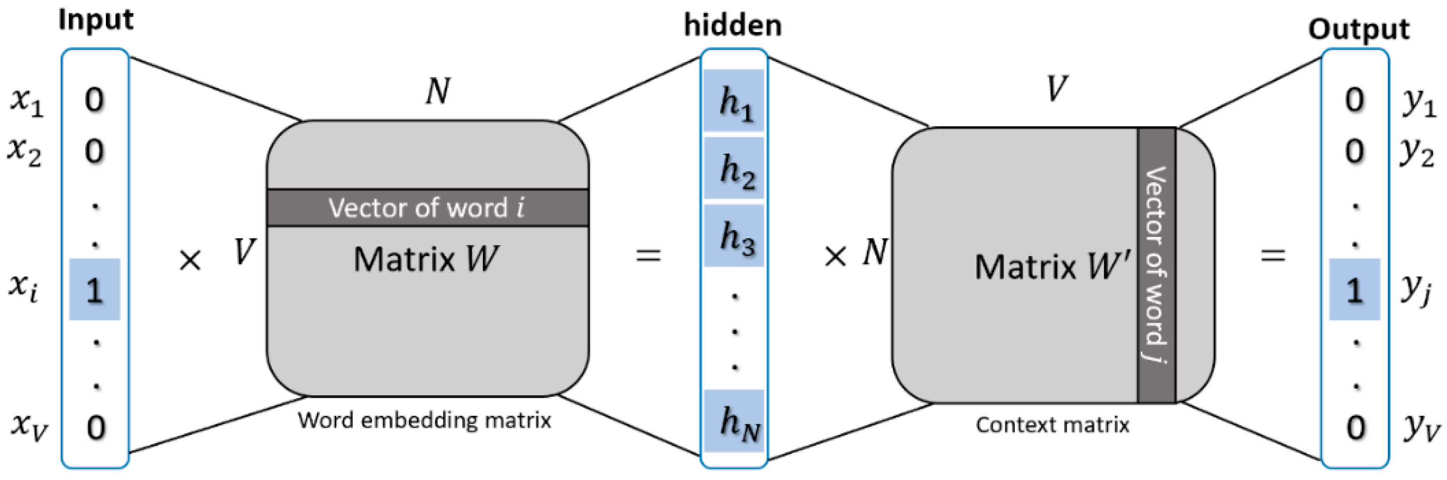
2.2. Word2vec

Word2vec [10] is a popular word-embedding approach and has many advantages compared to the earlier algorithms reported by Mikolov et al. [13]. Word2vec represents a word with a fixed-size vector. This vector is capable of effectively capturing semantic and syntactic similarities. For example, v(“queen”) − v(“woman”) + v(“man”) ≈ v(“king”) or v(“Thailand”) + v(“capital”) ≈ v(“Bangkok”). Word2vec is a prediction-based approach that trains from a large text corpus. Word2vec is one hidden layer artificial neural network. There are two models: Continuous bag-of-words (CBOW) and skip-gram. CBOW is given a context, then predicts a target word. However, skip-gram is just the mirror of CBOW; it is given a target word then predicts a context. In this paper, we will briefly describe the skip-gram only. The input of skip-gram is a single target word w_I, and the output is w_I’s context {w_O,1, w_O,2,…, w_O,C} defined by window size C. For example, we take the sentence, “I go to the bank to deposit money.” If a target word is “bank”, window size 4, stopword “to” and “the” are removed, the context will be “I go…deposit money.” The training instances, the input word, and the output words for the skip-gram model are formed with the following tuples: (“bank”, “I”), (“bank”, “go”), (“bank”, “deposit”), and (“bank”, “money”). Each word is encoded to one-hot vector size V. V is the size of the vocabulary. All positions will be “0”, except the position corresponding with the word which will be “1”. For example, in the vocabulary list (“I”, “go”, “bank”, “deposit”, “money”), the one-hot vector for “bank” is (0,0,1,0,0). These one-hot vectors are viewed as a column matrix with a size V × 1.

From Figure 1, x is a one-hot vector corresponding to the input word, and y is a probability vector corresponding to an output word in the training corpus. V × N matrix W is the weight matrix between the input layer and the hidden layer. Each row is a word-embedding vector size N that we will use to retrieve a word vector later. N is the training parameter of the model (i.e., dimensions of the word-embedding vectors). A hidden layer h is a multiplication matrix between one-hot vector x and matrix W with a size 1 × N, that makes the hidden layer h equivalent to matrix W row i which is mathematically expressed as Equation (1).

$$h=x^{T}W=W_{\left(i,·\right)}$$

(1)

N × V matrix W’ is a weight matrix between the hidden layer and the output layer. The output layer is a multiplication matrix between hidden layer h and weight matrix W’ with a size 1 × V, each component of the output layer is computed by Softmax classifier which produces the probability distribution represented by Equation (2).

$$\begin{gathered} u_j=h{W^{\prime }}_{\left(·,j\right)} \\ P\left(w_{O,j}|w_I\right)=y_j=\frac{exp\left(u_j\right)}{{{\displaystyle \sum }}_{j’=1}^{V}exp\left(u_{j’}\right)} \end{gathered}$$

(2)

Figure 1 illustrated only one training instance; actually, there are a bunch of training instances that can input to the model. The objective is to learn the weight W and W’ that minimizes the loss function (i.e., the difference between system outputs and output instances) by using backpropagation and the stochastic gradient descent algorithm [21]. There are many techniques involved in the training processes, such as subsampling frequent words and negative sampling [10,22,23]. After training, the word-embedding matrix W was used to retrieve a word vector.

3. Proposed Method

Our method used Word2vec instead of the LSA approach. Word2vec captures semantic and syntactic similarities better than the LSA approach when performing on a large corpus, as reported in Baroni et al. [11] and is more practical on real-world applications. We chose to use the signature of the word sense, which is the conjunction between the sense definition and its relationships (except “antonym” relationships) retrieved from WordNet. Sentence vectors were constructed from the sense signature and a context window using Word2vec with three different configurations, as will be detailed below. A score was calculated from cosine similarity; if the score was not higher than the specific threshold, the score would be combined with the probability of sense distribution. The possible answer senses can be obtained from high scores. The step-by-step procedure of our method is described below.

3.1. Constructing the Sentence Vector

In this paper, we are investigating three configurations of constructing the sentence vector. The first configuration is the summation of all word-embedding vectors. The sentence vector was constructed using Equation (3). W is a word list. |W| is the size of the word list. v(∙) is a Word2vec function. A word string was inputted to retrieve a corresponding word vector.

$$S={\displaystyle \sum }_{i=0}^{\left|W\right|}v\left(W\left[i\right]\right)$$

(3)

The second configuration is the average of all word-embedding vectors, which is just Equation (3) divided by the size of the word list. The sentence vector was redefined, as shown in Equation (4). Recently, the average of word-embedding vectors has proven to be a strong baseline in a multitude of tasks [24,25,26].

$$S=\frac{1}{\left|W\right|}{\displaystyle \sum }_{i=0}^{\left|W\right|}v\left(W\left[i\right]\right)$$

(4)

The third configuration is to weigh all word-embedding vectors according to the inverse document frequency (idf), promote rare terms, and demote frequent words, as in Equation (5). While t is a word, D is all documents in a corpus, |D| is the number of documents, and df(D,t) is the number of documents that containing word t.

$$idf\left(t,D\right){log}_{10}\frac{\left|D\right|}{df\left(D,t\right)}$$

(5)

Finally, the sentence vector was redefined as in Equation (6).

$$S=\frac{1}{\left|W\right|}{\displaystyle \sum }_{i=0}^{\left|W\right|}\left[v\left(W\left[i\right]\right)·idf\left(W\left[i\right],D\right)\right]$$

(6)

3.2. Cosine Similarity

The cosine similarity between two vectors was computed by their dot product divided by the product of their norm, as shown in Equation (7). The cosine similarity was in the range between 0 to 1. Two vectors were said to be similar when the cosine similarity was close to 1, and they were said to be dissimilar when it was close to 0 [27].

$$cosim\left(v_1,v_2\right)=\frac{v_1·v_2}{\Vert v_1\Vert \Vert v_2\Vert }$$

(7)

Our idea is that the correct word sense is likely to have a high cosine similarity with its context. Before doing this, all the word sense’s signatures and the context must be mapped to sentence vectors using the various configurations mentioned in the previous section.

3.3. The Probability of Sense Distribution

When context information is insufficient, cosine similarity fails to determine the correct word sense. Another idea also derived from intuition is that the correct word sense usually has a high probability of sense distribution. We adopted the same idea proposed in Basile et al. [6]. The probability of sense distribution was learned from SEMCOR [14], a large sense-tagged corpus annotated by WordNet, and it was defined as shown in Equation (8). C(w_i,s_i,j) counts the number of times w_i was tagged with sense s_i,j, C(w_i) counts the occurrences of w_i in the entire corpus, and C(s_i) counts the number of senses corresponding to w_i. Some senses do not occur in the corpus. The Laplace smoothing technique [28] has been used to avoid zero probabilities.

$$P\left(s_{i,j}│w_i\right)=\frac{C\left(w_i,s_{i,j}\right)+1}{C\left(w_i\right)+C\left(s_i\right)}$$

(8)

The score was combined between the cosine similarity and the probability of sense distribution when the score was not higher than the similarity threshold. The possible answer senses can be obtained from high scores. The similarity threshold is a system parameter which is further investigated in the next section.

3.4. Putting It Together

Algorithm 1 shows the pseudocode of the proposed method, wsdw2v. First, a sentence S, a target word w, a context size c, a similarity threshold α and a number of best synsets n_best must be given to a system. Line 1, the given sentence S is tokenized into a word list W. Each word is annotated with its part-of-speech tag. The stop words are removed from the word list W, and the remaining words are then lemmatized (i.e., a process of returning to the root word, e.g., eats → eat, ate → eat, eaten → eat). Line 2, scanning through the word list W to find the target word w and return a target word index w_i. Line 3, the context size c defines a number of words surrounding w_i. Therefore, context C consisted of a list of the following words {w_i-c/2,…,w_i-2,w_i-1,w_i+1,w_i+2,…,w_i+c/2} and then vectorized using Word2vec to V_C with Line 4. Line 5, a word senses inventory s_i (a set of synsets) is retrieved corresponding to w_i and its part-of-speech tag from WordNet. Line 6, set a variable Result to an empty dictionary. Line 8, set a variable Score to 0. Line 9, each word sense s_i,j (a synset) makes a signature sentence Sig by concatenating its definition and relations from WordNet. Line 10, the signature sentence Sig is also processed through tokenization, removing stop words, lemmatization and then vectorized using Word2vec to V_Sig with Line 11. Line 12, the context sentence vector V_C and the signature sentence vector V_sig are then used to compute the variable Score from cosim(V_C, V_sig). Line 13, if the variable Score is not higher than the similarity threshold α, it will be combined with the probability of sense distribution P(s_i,j│w_i) with Line 14 and the variable Result is appended with a dictionary entry {s_i,j : Score} with Line 15. After all word senses are processed, n_best senses (the synsets) are returned according to their scores as an output of the system with Line 16. The context size c and the similarity threshold α are a system parameter which is to further investigated in the next section. Figure 2 shows some examples of wsdw2v (Jupyter notebook for wsdw2v is available at https://anaconda.org/korawit/wsdw2v/notebook) to disambiguate word “bank” and “plant” in different contexts. The answer senses for each example are ranked by their scores.

Algorithm 1 Pseudocode of proposed method, wsdw2v

Input: a sentence S, a target word w, a context size c, a similarity threshold α, a number of best synsets n_best Output: n_best disambiguate senses (synsets) of the target word w 1: W←Lemmatized(RemoveStopwords(POStag(Tokenized(S)))) 2: wi←GetTargetWordIndex(W, w) 3: C←GetContext(W, wi, c) 4: VC←Word2Vectorizer(C) 5: si←GetSynsetsFromWordNet(wi, GetPOStag(wi)) 6: Result←EmptyDict() 7: For each synset si,j in si : 8:   Score←0 9:   Sig←GetDefinition(si,j)+GetDefinitionFromRelations(si,j, “hypernym, hyponym, meronym, holonym, entailment”) 10:  Sig←Lemmatized(RemoveStopwords(Tokenized(Sig)))

11:  VSig←Word2Vectorizer(Sig) 12:  Score←Cosim(VC, VSig) 13:  If Score < α : 14:    Score←P(si,j|wi) 15:  Result←Result + {si,j : Score} 16: Return n_best synsets from Result

In order to enhance the scalability of the method when analyzing a bunch of documents, it is possible that some word senses have been retrieved several times from WordNet. The method could be extended to store these word senses in a cache as the vectorized form. Next time when these word senses were found, the method could retrieve the respective vectorized forms directly from the cache. This extended method needs to pay off some overheads (i.e., disk space) to increase overall performance. Another scalability is that the method could be integrated with a user-defined dictionary or other public lexicons/dictionaries [19] to cover more words.

4. Experiments and Results

Our method (wsdw2v evaluated with senseval-3 is available at https://anaconda.org/korawit/project/wsdw2v_source) was evaluated using a SENSEVAL-3 English lexical sample task [15]. A part-of-speech tagged text corpus providing specifying 2040 question words corresponding to their correct word senses [29]. Our method was set to return only one best synset as an answer sense (n_best = 1). We adopted a scoring method (precision and recall) proposed by Resnik and Yarowsky [30] in Section 3.1 of their work [31]. The precision of a system is computed by summing the scores overall question words that the system handles and dividing by the number of handle question words. The recall of the system is computed by summing the scores of the overall question words (counting unhandled question words as a zero score) and dividing by the number of all question words. Our method did not handle the question words in two cases: (1) The question words not in WordNet (52 question words) and (2) the question words that could not define the correct sense based on WordNet synsets (34 question words), so our method handled only 1954 question words. All experiments were written using the python programming language (pre-installed NLTK [32], scikit-learn library [33], and Gensim [34]) and run under Window 10 Pro, Intel Core i5-6500 CPU 3.20 GHz, and a RAM of 16 GB (Harbin, China). Experiments were conducted in various configurations as will be detailed below.

4.1. Training Word-Embedding Vectors

In this paper, we used 300 dimensions of pre-trained word-embedding vectors [35] from Google News Dataset. This comprised of around 100 billion words, which provided three million word-embedding vectors that promise 77.1% accuracy for 20,000 word analogy test examples [36]. This test follows an “A is to B as C is to D” scheme. For example, “Bangkok is to Thailand as Beijing is to China,” which can be tested by v(“Bangkok”) + v(“China”) − v(“Thailand”) ≈ v(“Beijing”). Unfortunately, pre-trained word-embedding vectors from Google did not provide their dataset. We could not compute the inverse document frequency. Therefore, we decided to train our word-embedding vectors from the UMBC (University of Maryland, Baltimore County) WebBase Corpus [37,38], containing over three billion words which provided around five million word-embedding vectors. The training was done using Gensim with the same parameters as Google word-embedding vectors, which achieved 69% accuracy on word analogy test examples. UMBC word-embedding vectors were used to evaluate three configurations of constructing a sentence vector. Training time for UMBC word-embedding vectors was 460 min and using overall memory 10,538 MB. We also trained an LSA model from the UMBC WebBase Corpus about four million documents with 100,000 most shared features and reduced dimensions to 200. We used this LSA model to compare with our method, wsdw2v. Training time for the LSA model was 174 min and using overall memory 101,220 MB. Notice that the LSA model took much more memory than the Word2vec model. In order to train a model from a large corpus, physical memory may be not sufficient to hold large data structures. Thus, many operating systems provide a memory management technique called virtual memory that moves some data from physical memory to a paging file on disk storages. We used this virtual memory technique in case of training the LSA model because overall memory could not fit with our physical memory (a RAM of 16 GB).

4.2. Determining Similarity Threshold

A similarity threshold is a cut-off point to classify whether they are similar or not. The similarity threshold behaves differently based on the vector space model and system domain structure. In our method (Jupyter notebook is available at https://anaconda.org/korawit/similarity_threshold/notebook), we approximately select the similarity threshold based on a predictive model validated by a human with the following steps: (1) Randomly select a small sample of questions (i.e., pairs of context and signature.) (2) Compute cosine similarity score for each question using wsdw2v. (3) Each question is given a binary score (1 if relevant, 0 if not relevant) whether it is relevant between context and signature by a human without seeing its cosine similarity score. (4) Using a logistic regression model [39] by input cosine similarity scores and binary scores as true labels, then fitting the model by minimizing differences between true labels and predicted labels (we used scikit-learn library to create and fit the logistic regression model.) (5) The logistic regression model can now predict a probability of relevance given a cosine similarity score. Input all cosine similarity scores again into the model and predict probabilities of relevance, sort all cosine similarity scores and corresponding probabilities of relevance by descending order, then select a cosine similarity score at 0.5 of the probability of relevance as an empirical similarity threshold. In our case, we found that 0.37 was the empirical similarity threshold of our method. We will use 0.37 as the similarity threshold throughout the paper. If the cosine similarity score below this threshold means that the contextual similarity might fail to determine the correct word sense, the score will be calculated from the probability of sense distribution instead. Set too high similarity threshold only the word sense that has almost identical context and signature, can be scored. The score is more likely to compute from the probability of sense distribution. On the other hand, set too low similarity threshold allows the word sense that has less similar context and signature, can be scored. The score is more likely to be computed from cosine similarity rather than the probability of sense distribution.

4.3. Experiment on Sense Relations and Sense Distribution

In this experiment, we wanted to know whether sense relationships/sense distribution affected the results. We used Google word-embedding vectors to construct a sentence vector using the average of the word-embedding vectors as a baseline. We selected the context size of ten, which is in the middle of the range of 2–14. When not combining with sense distribution, the similarity threshold (α) is 0; otherwise, the similarity threshold (α) is 0.37 and n_best = 1.

From

Table 3. The results with and without sense relationships/sense distribution.

Configurations	Sense Distribution	Precision	Recall
Sense definition	×	0.421	0.403
Sense definition + sense relations	×	0.487	0.466
Sense definition	√	0.480	0.459
Sense definition + sense relations	√	0.509	0.488

, the results show that sense relations significantly affect the results and, when combined with the probability of sense distribution, the results have been improved a little bit.

4.4. Experiment on Context Size

The context size is the number of words surrounding a target word which is a system parameter. This experiment aims to determine whether the context size affects the result. Experimental context sizes were within a range of 2–14, with intervals of two. We used the best configurations from the previous experiment, i.e., the sense signature (sense definition and sense relations) without the probability of sense distribution using the average of Google word-embedding vectors as the baseline and n_best = 1.

From

Table 4. The results of different context sizes.

Configurations	Precision	Recall
Context size 2	0.446	0.427
Context size 6	0.455	0.436
Context size 10	0.487	0.466
Context size 14	0.471	0.451

, the results show that the context size slightly affects the results. Providing a few context words or many context words slightly harms the results. The middle context size is recommended to get the best result.

4.5. Experiment on Constructing a Sentence Vector

This experiment aims to determine which configuration is the best for constructing a sentence vector. There are three configurations: (1) The summation of word-embedding vectors, (2) the average of word-embedding vectors, and (3) the average of the word-embedding vectors with inverse document frequency (idf). We needed to compute idf, so we used our own UMBC word-embedding vectors. This experiment used the best configurations (i.e., context size of ten, sense definition and sense relations, n_best = 1) from the previous experiment without the probability of sense distribution feature to show the actual effect of each configuration.

From

Table 5. The results of different configurations for constructing a sentence vector.

Configurations	Precision	Recall
Summing word-embedding vectors	0.417	0.399
Average word-embedding vectors	0.417	0.399
Average word-embedding vectors + idf	0.416	0.398

, the result shows that using the summation of word-embedding vectors or the average of word-embedding vectors provides the same result. Because cosine similarity only measures the direction of the vector, dividing or multiplying a scalar to the resultant word vector affects only the magnitude of the vector and not its direction, except for zero scalars which cancel that word vector out of the sentence vector. Idf was not useful in WSD, for example, a word sense “university” and the context contained a term “student,” because of the term “student” appeared most frequently in the UMBC corpus; thus it got demoted and made it less significant to help in disambiguation for word sense “university.” Notice that results from Google word-embedding vectors (48.7%) were better than UMBC word-embedding vectors (41.7%) because Google word-embedding vectors were trained from a larger dataset. Hence, it will be possible to obtain more accuracy by training word vectors from a larger dataset than the Google News Dataset, but it will require more training time and resources.

4.6. Comparing with Other Systems

From

Table 6. Performance of unsupervised systems participating in the SENSEVAL-3 English lexical sample task compared with our method and baselines.

System/Team	Precision	Recall
wsdiit/IIT Bombay (Ramakrishnan et al.)	0.661	0.657
Cymfony/(Niu)	0.563	0.563
the “most frequent sense” heuristic-baseline	0.552	0.552
Prob0/Cambridge U. (Preiss)	0.547	0.547
wsdw2v with sense distribution (our method)	0.509	0.488
wsdw2v without sense distribution (our method)	0.487	0.466
clr04-ls/CL Research (Litkowski)	0.450	0.450
CIAOSENSO/U. Genova (Buscaldi)	0.501	0.417
LSA Lesk	0.408	0.408
KUNLP/Korea U. (Seo)	0.404	0.404
Duluth-SenseRelate/U.Minnesota (Pedersen)	0.403	0.385
Simplified Lesk (Kilgarriff and Rosenzweig)	0.311	0.298
Adapted Lesk (Banerjee and Pederson)	0.247	0.236
DFA-LS-Unsup/UNED (Fernandez)	0.234	0.234
DLSI-UA-LS-NOSU/U.Alicante (Vazquez)	0.197	0.117
Original Lesk (M. Lesk)	0.097	0.053

, a short description for each system is given as follows (same as Table 3 in [15]). Wsdiit is an unsupervised system using a Lesk-like similarity between the contexts of ambiguous words and dictionary definitions. Experiments were performed for various window sizes and various similarity measures. Cymfony is a maximum entropy model for unsupervised clustering and using nearby words and syntactic structures as features. A few annotated instances were used to map context clusters to WordNet/Worsmyth senses. Prob0 is a combination of two unsupervised modules using basic parts-of-speech tag and frequency information. Wsdw2v (our method) uses Word2vec to construct a context sentence vector and sense signatures’ sentence vectors retrieved from WordNet, computing the cosine similarity between those sentence vectors combined with the probability of sense distribution (using the average of Google word-embedding vectors, context = 10, similarity threshold α = 0.37, n_best = 1). Clr04-ls is an unsupervised system relying on definition properties (e.g., syntactic, semantic, subcategorization patterns, other lexical information), as given in a dictionary. Performance is generally a function of how well senses are distinguished. CIAOSENSO is an unsupervised system that combines the conceptual density idea with the frequency of words to disambiguate them. Information about domains was also taken into account. KUNLP is an algorithm that disambiguates the senses of a word by selecting a substituent among its WordNet relatives (e.g., antonyms KUNLP, hypernyms, etc.). The selection was made based on co-occurrence frequencies, measured on a large corpus. Duluth-SenseRelate is an algorithm that assigns the sense to a word that is most related to the possible senses of its neighbors, using WordNet glosses to measure relatedness between senses. DFA-LS-Unsup is a combination of three heuristics: the similarity between synonyms and the context, according to a mutual information measure; lexico-syntactic patterns extracted from WordNet glosses; and the first sense heuristic. DLSI-UA-LS-NOSU is an unsupervised method based on WordNet domains [40]; it exploits the information contained in glosses of WordNet domains and uses “Relevant Domains” obtained from the association ratio over domains and words.

For the baselines, “most frequent sense” heuristic baseline is known as a very hard baseline to outperform by unsupervised WSD algorithms. The original Lesk computes overlapping words between each pair of word sense definitions. The simplified Lesk computes overlapping words between word sense definitions and the context word instead. The adapted Lesk extends a sense definition with sense relations. LSA Lesk makes a model analyzing distributional semantic relationships between a set of documents and terms in documents from a large text corpus, and converts a context and sense signatures using the model to vectorial forms then computing similarity using cosine similarity. The results show that our method (50.9% or 48.7% without the probability of sense distribution) outperforms many baselines (i.e., original Lesk–9.7%, simplified Lesk–31.1%, adapted Lesk–24.7%, and LSA Lesk–40.8%) and many unsupervised systems participating in SESEVAL-3 English lexical sample task.

Notice that wsdiit gives better performance compared to wsdw2v (our method) because wsdw2v uses only the cosine similarity, but wsdiit uses various similarity measures. So, our method could benefit from using other similarity measures [41] as well. Another reason is that some words that cannot be retrieved from Word2vec, although the Google News Dataset provides 3,000,000 word-embedding vectors but does not cover all the words in WordNet. This problem affected the results as well. Training word-embedding vectors from bigger datasets could solve this problem but, on the other hand, it requires more training time and resources (e.g., CPU and RAM). It could also be solved by using other word-embedding approaches [42,43,44] that can handle out of dictionary issues.

5. Example of Applications

Sentiment analysis [45,46] is one of many NLP applications using WSD. Sentiment analysis is to identify the subjective information that reflects people’s opinions, attitudes, and feelings regarding something or someone. Each word has different polarity scores depending on its sense. For example, the word “breakdown” in the context of “a mental or physical breakdown” conveys negative polarity whereas “breakdown” in the context of “an analysis into mutually exclusive categories” conveys no polarity. The instant way to retrieve polarity scores is from a lexicon resource for sentiment analysis and opinion mining called SentiWordNet [47] by providing it, the correct sense (the synset from WordNet) as an input. SentiWordNet developed based on quantitative analysis of the definitions associated with the synsets and semi-supervised classifications. Training dataset started with a small amount of manual annotation and then using WordNet to crawl along the associated synsets for bootstrapping training dataset. Three numerical scores (i.e., objective score, positive score, and negative score) are produced by combining the results of a committee of eight ternary classifications. SentiWordNet is reported as an efficiently performing lexical resource for sentiment analysis of microblog posts [48]. Therefore, WSD is the important pre-processing step, and its accuracy directly affects the result of lexicon-based sentiment analysis. WSD and SentiWordNet have been used in many research works related with social media analytics [49], e.g., Chamlertwat et al. [50] discovered insights from Twitter by sentiment analysis, Hamzehei et al. [51] proposed a scalable semantic-based sentiment analysis methodology.

Moreover, WSD could be employed in the feature extraction process for supervised machine learning approaches, e.g., in this work, “Beyond Binary Labels: Political Ideology Prediction of Twitter Users” [52]. They used a broad range of linguistic features to help in prediction; one of them is the sentiment and emotion feature by quantifying emotion terms from Twitter posts using lexicon of words associated with six basic emotions (i.e., anger, disgust, fear, joy, sadness, and surprise) as well as general positive and negative sentiment. As mentioned earlier, words have different meanings and also convey different sentiment orientations. WSD could help in the process to automatically obtain the correct sentiment orientation of the terms relying on the context. WSD could help in data collection and preprocessing as well; e.g., in “Fortune Teller: Predicting Your Career Path” [53], they manually collected information about careers by searching for keywords corresponding to the career paths from different social network accounts such as Twitter, Facebook and Linkedin, grouped similar careers and then predicted a career path. WSD can distinguish different careers automatically. For example, with the keyword “doctor”, there are two-word senses associated with career “doctor”: i.e., a licensed medical practitioner and a person who holds a Ph.D. degree. WSD will group similar social network accounts by computing the similarity between the curriculum vitae and word sense definitions.

6. Conclusions and Future Works

WSD is an important task for many NLP applications. Our method is derived from the intuitive idea that the correct sense most likely has a high similarity between the sense definition retrieved from WordNet and its context. Sense relations are also included to provide more information. Instead of using an overlap-based approach, we constructed sentence vectors from a popular word-embedding approach, Word2vec, which is capable of effectively capturing semantic and syntactic similarities better than the LSA approach when dealing with a huge corpus of text and using less memory. Cosine similarity was used to compute between those two sentence vectors. If context did not help in disambiguation, the cosine similarity score was below the empirical similarity threshold 0.37 (estimated by the logistic regression model and validated by a human), the probability of sense distribution learned from a large sense-tagged corpus, SEMCOR, was also combined with the result. The possible answer senses were obtained from high scores. The experiments were conducted to verify that the sense relations and sense distribution were useful to help WSD gain more accuracy. Moreover, experiments were conducted in various context sizes and various constructing sentence vector configurations. The results show that the middle context size is recommended and that it gives the same result no matter whether summation or average word-embedding was used to construct a sentence vector; however, idf was not useful in WSD. The size of the corpus that the word-embedding vectors trained from affects accuracy as well. The result shows that our method wsdw2v, (50.9% or 48.7% without the probability of sense distribution) is higher than the baselines (i.e., original, simplified, adapted and LSA Lesk) and outperforms many unsupervised systems participating in the SENSEVAL-3 English lexical sample task. Our method could benefit from using other similarity measures [41] or using other sentences, phrases, or word-embedding approaches [42,43,44] and also could benefit from integrating with other lexicon resources such as BabelNet [19].

References

- Zhong, Z.; Ng, H.T. It Makes Sense: A Wide-Coverage Word Sense Disambiguation System for Free Text. In Proceedings of the ACL 2010 System Demonstrations, Uppsala, Sweden, 13 July 2010; pp. 78–83. [Google Scholar]
- Lesk, M. Automatic Sense Disambiguation Using Machine Readable Dictionaries: How to Tell a Pine Cone from an Ice Cream Cone. In Proceedings of the 5th Annual International Conference on Systems Documentation, Toronto, ON, Canada, January 1986; pp. 24–26. [Google Scholar]
- Cowie, J.; Guthrie, J.; Guthrie, L. Lexical Disambiguation Using Simulated Annealing. In Proceedings of the 14th conference on Computational linguistics-Volume 1, Nantes, France, 23–28 August 1992; Association for Computational Linguistics: Stroudsburg, PA, USA, 1992; pp. 359–365. [Google Scholar]
- Kilgarriff, A.; Rosenzweig, J. Framework and Results for English SENSEVAL. Comput. Humanit. 2000, 34, 15–48. [Google Scholar] [CrossRef]
- Banerjee, S.; Pedersen, T. An Adapted Lesk Algorithm for Word Sense Disambiguation Using WordNet. In Proceedings of the International Conference on Intelligent Text Processing and Computational Linguistics, Mexico City, Mexico, 17–23 February 2002; pp. 136–145. [Google Scholar]
- Basile, P.; Caputo, A.; Semeraro, G. An Enhanced Lesk Word Sense Disambiguation Algorithm through a Distributional Semantic Model. In Proceedings of the COLING 2014, 25th International Conference on Computational Linguistics: Technical Papers, Dublin, Ireland, 23–29 August 2014; pp. 1591–1600. [Google Scholar]
- Yarowsky, D. Unsupervised Word Sense Disambiguation Rivaling Supervised Methods. In Proceedings of the 33rd Annual Meeting on Association for Computational Linguistics, Cambridge, MA, USA, 26–30 June 1995; Association for Computational Linguistics, 1995; pp. 189–196. [Google Scholar]
- Miller, G. WordNet: An Electronic Lexical Database; MIT press: Cambridge, MA, USA, 1998. [Google Scholar]
- Landauer, T.K.; Foltz, P.W.; Laham, D. An Introduction to Latent Semantic Analysis. Discourse Process. 1998, 25, 259–284. [Google Scholar] [CrossRef]
- Mikolov, T.; Sutskever, I.; Chen, K.; Corrado, G.S.; Dean, J. Distributed Representations of Words and Phrases and Their Compositionality. In Proceedings of the Advances in Neural Information Processing Systems (NIPS 2013), Lake Tahoe, NV, USA, 5–8 December 2013; pp. 3111–3119. [Google Scholar]
- Baroni, M.; Dinu, G.; Kruszewski, G. Don’t Count, Predict! A Systematic Comparison of Context-Counting vs. Context-Predicting Semantic Vectors. In Proceedings of the 52nd Annual Meeting of the Association for Computational Linguistics (Volume 1: Long Papers), Baltimore, MD, USA, 23–25 June 2014; Volume 1, pp. 238–247. [Google Scholar]
- Altszyler, E.; Sigman, M.; Ribeiro, S.; Slezak, D.F. Comparative Study of LSA vs Word2vec Embeddings in Small Corpora: A Case Study in Dreams Database. arXiv 2016, arXiv:1610.01520. [Google Scholar]
- Mikolov, T.; Chen, K.; Corrado, G.; Dean, J. Efficient Estimation of Word Representations in Vector Space. arXiv 2013, arXiv:1301.3781. [Google Scholar]
- Mihalcea, R.; (University of Michigan, Michigan, USA). Semcor Semantically Tagged Corpus. Unpublished manuscript. 1998. [Google Scholar]
- Mihalcea, R.; Chklovski, T.; Kilgarriff, A. The Senseval-3 English Lexical Sample Task. In Proceedings of the SENSEVAL-3, the Third International Workshop on the Evaluation of Systems for the Semantic Analysis of Text, Barcelona, Spain, 25–26 July 2004. [Google Scholar]
- Vasilescu, F.; Langlais, P.; Lapalme, G. Evaluating Variants of the Lesk Approach for Disambiguating Words. In Proceedings of the Fourth International Conference on Language Resources and Evaluation (Lrec’04), Lisbon, Portugal, 26–28 May 2004. [Google Scholar]
- Edmonds, P.; Cotton, S. SENSEVAL-2: Overview. In Proceedings of the Second International Workshop on Evaluating Word Sense Disambiguation Systems, SENSEVAL ’01, Toulouse, France, 5–6 July 2001; Association for Computational Linguistics: Toulouse, France, 2001; pp. 1–5. [Google Scholar]
- Mihalcea, R.; Tarau, P.; Figa, E. PageRank on Semantic Networks, with Application to Word Sense Disambiguation. In Proceedings of the 20th International Conference on Computational Linguistics, Geneva, Switzerland, 23–27 August 2004; Association for Computational Linguistics, 2004; p. 1126. [Google Scholar]
- Navigli, R.; Ponzetto, S.P. BabelNet: The Automatic Construction, Evaluation and Application of a Wide-Coverage Multilingual Semantic Network. Artif. Intell. 2012, 193, 217–250. [Google Scholar] [CrossRef]
- Navigli, R.; Jurgens, D.; Vannella, D. Semeval-2013 Task 12: Multilingual Word Sense Disambiguation. In Proceedings of the Second Joint Conference on Lexical and Computational Semantics (* SEM), Volume 2 and the Seventh International Workshop on Semantic Evaluation (SemEval 2013), Atlanta, GA, USA, 14–15 June 2013; Volume 2, pp. 222–231. [Google Scholar]
- Amari, S. Backpropagation and Stochastic Gradient Descent Method. Neurocomputing 1993, 5, 185–196. [Google Scholar] [CrossRef]
- Gutmann, M.; Hyvärinen, A. Noise-Contrastive Estimation of Unnormalized Statistical Models, with Applications to Natural Image Statistics. J. Mach. Learn. Res. 2012, 13, 307–361. [Google Scholar]
- Mnih, A.; Whye Teh, Y. A Fast and Simple Algorithm for Training Neural Probabilistic Language Models. In Proceedings of the 29th International Conference on Machine Learning, ICML 2012, Edinburgh, UK, 26 June–1 July 2012. [Google Scholar]
- Faruqui, M.; Dodge, J.; Kumar Jauhar, S.; Dyer, C.; Hovy, E.; Smith, N.A. Retrofitting Word Vectors to Semantic Lexicons. In Proceedings of the Human Language Technologies: The 2015 Annual Conference of the North American Chapter of the ACL, Denver, CO, USA, 31 May–5 June 2014; pp. 1606–1615. [Google Scholar]
- Yu, L.; Moritz Hermann, K.; Blunsom, P.; Pulman, S. Deep Learning for Answer Sentence Selection. In Proceedings of the Deep Learning and Representation Learning Workshop: NIPS-2014, Montréal, QC, Canada, 8–13 December 2014. [Google Scholar]
- Kenter, T.; de Rijke, M. Short Text Similarity with Word Embeddings. In Proceedings of the 24th ACM International on Conference on Information and Knowledge Management, Melbourne, Australia, 18–23 October 2015; pp. 1411–1420. [Google Scholar]
- Singhal, A.; Google, I. Modern Information Retrieval: A Brief Overview. IEEE Data Eng. Bull. 2001, 24, 35–43. [Google Scholar]
- Manning, C.D.; Raghavan, P.; Schütze, H. Introduction to Information Retrieval; Cambridge University Press: New York, NY, USA, 2008. [Google Scholar]
- SENSEVAL 3 Home Page. Available online: http://web.eecs.umich.edu/~mihalcea/senseval/senseval3/data.html (accessed on 10 November 2018).
- Resnik, P.; Yarowsky, D. A Perspective on Word Sense Disambiguation Methods and Their Evaluation. In Tagging Text with Lexical Semantics: Why, What, and How? Washington, WA, USA, 4–5 April 1997, pp. 79–86.
- Proposal for Senseval Scoring Scheme. Available online: http://web.eecs.umich.edu/~mihalcea/senseval/senseval3/scoring/scorescheme.txt (accessed on 15 November 2018).
- Wagner, W. Steven Bird, Ewan Klein and Edward Loper: Natural Language Processing with Python, Analyzing Text with the Natural Language Toolkit. Lang. Resour. Eval. 2010, 44, 421–424. [Google Scholar] [CrossRef]
- Pedregosa, F.; Varoquaux, G.; Gramfort, A.; Michel, V.; Thirion, B.; Grisel, O.; Blondel, M.; Prettenhofer, P.; Weiss, R.; Dubourg, V.; et al. Scikit-Learn: Machine Learning in Python. J. Mach. Learn. Res. 2011, 12, 2825–2830. [Google Scholar]
- Řehůřek, R.; Sojka, P. Software Framework for Topic Modelling with Large Corpora. In Proceedings of the LREC 2010 Workshop on New Challenges for NLP Frameworks, Valletta, Malta, 22 May 2010; ELRA: Valletta, Malta, 2010; pp. 45–50. [Google Scholar]
- Google Code Archive: word2vec. Available online: https://code.google.com/archive/p/word2vec/ (accessed on 9 October 2018).
- Word Analogies Test for word2vec. Available online: https://raw.githubusercontent.com/RaRe-Technologies/gensim/develop/gensim/test/test_data/questions-words.txt (accessed on 9 October 2018).
- Han, L. UMBC Webbase Corpus. Available online: https://ebiquity.umbc.edu/resource/html/id/351 (accessed on 21 October 2018).
- Han, L.; Kashyap, A.L.; Finin, T.; Mayfield, J.; Weese, J. UMBC_EBIQUITY-CORE: Semantic Textual Similarity Systems. In Proceedings of the Second Joint Conference on Lexical and Computational Semantics, Atlanta, Georgia, USA, 13–14 June 2013; Association for Computational Linguistics, 2013. [Google Scholar]
- Hilbe, J.M. Logistic Regression Models; Chapman and Hall/CRC: Boca Raton, FL, USA, 2009. [Google Scholar]
- Magnini, B.; Strapparava, C. User Modelling for News Web Sites with Word Sense Based Techniques. User Model. User-Adapt. Interact. 2004, 14, 239–257. [Google Scholar] [CrossRef]
- Sidorov, G.; Gelbukh, E.; Pinto, D. Soft Similarity and Soft Cosine Measure: Similarity of Features in Vector Space Model. Computación y Sistemas 2014, 18, 491–504. [Google Scholar] [CrossRef]
- Le, Q.; Mikolov, T. Distributed Representations of Sentences and Documents. In Proceedings of the 31st International Conference on Machine Learning, Beijing, China, 22–24 June 2014. [Google Scholar]
- Pennington, J.; Socher, R.; Manning, C.D. Glove: Global Vectors for Word Representation. In Proceedings of the 2014 Conference on Empirical Methods in Natural Language Processing (EMNLP), Doha, Qatar, 25–29 October 2014; pp. 1532–1543. [Google Scholar]
- Bojanowski, P.; Grave, E.; Joulin, A.; Mikolov, T. Enriching Word Vectors with Subword Information. arXiv 2016, arXiv:1607.04606. [Google Scholar] [CrossRef]
- Yu, H.; Hatzivassiloglou, V. Towards Answering Opinion Questions: Separating Facts from Opinions and Identifying the Polarity of Opinion Sentences. In Proceedings of the 2003 Conference on Empirical Methods in Natural Language Processing, Sapporo, Japan, 11–12 July 2003; Association for Computational Linguistics, 2003; pp. 129–136. [Google Scholar]
- Kim, S.-M.; Hovy, E. Determining the Sentiment of Opinions. In Proceedings of the 20th international conference on Computational Linguistics, Geneva, Switzerland, 23–27 August 2004; Association for Computational Linguistics, 2004; p. 1367. [Google Scholar]
- Baccianella, S.; Esuli, A.; Sebastiani, F. Sentiwordnet 3.0: An Enhanced Lexical Resource for Sentiment Analysis and Opinion Mining. In Proceedings of the Seventh conference on International Language Resources and Evaluation (LREC’10), Valletta, Malta, 17–20 May 2010; Volume 10, pp. 2200–2204. [Google Scholar]
- Musto, C.; Semeraro, G.; Polignano, M. A Comparison of Lexicon-Based Approaches for Sentiment Analysis of Microblog Posts. In Proceedings of the 8th International Workshop on Information Filtering and Retrieval, Pisa, Italy, 10 December 2014; pp. 59–69. [Google Scholar]
- Batrinca, B.; Treleaven, P.C. Social Media Analytics: A Survey of Techniques, Tools and Platforms. AI & Soc. 2015, 30, 89–116. [Google Scholar]
- Chamlertwat, W.; Bhattarakosol, P.; Rungkasiri, T.; Haruechaiyasak, C. Discovering Consumer Insight from Twitter via Sentiment Analysis. J. UCS 2012, 18, 973–992. [Google Scholar]
- Hamzehei, A.; Ebrahimi, M.; Shafiee, E.; Wong, R.K.; Chen, F. Scalable Sentiment Analysis for Microblogs Based on Semantic Scoring. In Proceedings of the 2015 IEEE International Conference on Services Computing, New York, NY, USA, 27 June–2 July 2015; pp. 271–278. [Google Scholar]
- Preoţiuc-Pietro, D.; Liu, Y.; Hopkins, D.; Ungar, L. Beyond Binary Labels: Political Ideology Prediction of Twitter Users. In Proceedings of the 55th Annual Meeting of the Association for Computational Linguistics (Volume 1: Long Papers), Vancouver, BC, Canada, 30 July–4 August 2017; Association for Computational Linguistics: Vancouver, BC, Canada, 2017; pp. 729–740. [Google Scholar] [CrossRef]
- Liu, Y.; Zhang, L.; Nie, L.; Chen, Y.; Rosenblum, D.S. Fortune Teller: Predicting Your Career Path. In Proceedings of the Thirtieth AAAI Conference on Artificial Intelligence (AAAI’16), Phoenix, AZ, USA, 12–17 February 2016; pp. 201–207. [Google Scholar]