Real-Time Monitoring of Passenger’s Psychological Stress
by
 , , and
Gaël Vila
1 ,
,
Christelle Godin
1,*,
Oumayma Sakri
1,
Etienne Labyt
1,
Audrey Vidal
1,
Sylvie Charbonnier
2,
Simon Ollander
1 and
Aurélie Campagne
3 1
Univ. Grenoble Alpes & CEA, LETI, MINATEC Campus, F-38054 Grenoble, France
2
Gipsa-Lab, Univ. Grenoble Alpes & CNRS, F-38402 Grenoble, France
3
Univ. Grenoble Alpes, CNRS, LPNC, 38000 Grenoble, France
*
Author to whom correspondence should be addressed.
Future Internet 2019, 11(5), 102; https://doi.org/10.3390/fi11050102
Submission received: 29 March 2019
/
Revised: 20 April 2019
/
Accepted: 24 April 2019
/
Published: 26 April 2019
(This article belongs to the Special Issue Internet of Things for Smart City Applications)
Abstract
:This article addresses the question of passengers’ experience through different transport modes. It presents the main results of a pilot study, for which stress levels experienced by a traveller were assessed and predicted over two long journeys. Accelerometer measures and several physiological signals (electrodermal activity, blood volume pulse and skin temperature) were recorded using a smart wristband while travelling from Grenoble to Bilbao. Based on user’s feedback, three events of high stress and one period of moderate activity with low stress were identified offline. Over these periods, feature extraction and machine learning were performed from the collected sensor data to build a personalized regressive model, with user’s stress levels as output. A smartphone application has been developed on its basis, in order to record and visualize a timely estimated stress level using traveler’s physiological signals. This setting was put on test during another travel from Grenoble to Brussels, where the same user’s stress levels were predicted in real time by the smartphone application. The number of correctly classified stress-less time windows ranged from 92.6% to 100%, depending on participant’s level of activity. By design, this study represents a first step for real-life, ambulatory monitoring of passenger’s stress while travelling.
1. Introduction
1.1. General Background and Motivations
Stress is an umbrella term for some psychological, physiological and behavioral response to environmental factors we perceive as a potential threat. In the short run, it should boost our ability to cope with this kind of stimuli: stress hormones are released in the body and the sympathetic nervous system has increased activity [1], bringing the entire organism in a general state of alarm. When the threatening stimulus is repeated or lasts over too much time, acute stress (the natural emotional response) becomes chronic, and may turn into mental disorders. From a psychological viewpoint, the recurrence of too many daily hassles is a threat to an individual’s wellbeing [2]. From a clinical viewpoint, it may have heavy impacts on health [1].
Stressful events (or surroundings) are frequently encountered during daily urban trips. In the middle 1980s, an extensive survey based on people’s answers to a detailed questionnaire tried to quantify the phenomenon [3]. Participants included 1167 Italian workers, and 437 Dutch people who worked in the production unit of a heavy engineering company. Part of these people went through long commuting distances from home to the working place. Regarding the Italian people, experimenters found significantly higher scores in chronic psychological stress for the commuting people than for non-commuters. Those people also demonstrated more complaints, illnesses and absenteeism due to sickness. Similarly, the Dutch commuters showed a significant increase in stress disorders (tiredness, edginess, irritability, lack of concentration and difficulty in sleeping) compared to the non-commuting Dutch people. This increase was only a trend for non-production workers, suggesting that stress disorders due to everyday travels are widespread but worsen with poorer living standards.
In a broader context, it has been shown that different travelling options have distinct effects on passengers’ stress and mood [4]. For example, perceived crowding appears a major cause of discomfort among train passengers, and therefore increases their psychological stress [5]. Stress and mood during a journey are also mediated by a host of factors, like comfort and effort, with respect to the individual, or control and predictability, regarding their environment [5,6]. This relationship is very similar to the one found in the working medium: that is why stress experienced by frequent travellers have sometimes been compared to actual job strain [3]. An objective feedback on passengers’ mental states would enable smart environments to adapt and increase people’s ability to cope with every hassle of a daily trip—and thus help prevent chronic stress onset.
Since acute stress has short-term physiological correlates (e.g., sympathetic activation), various peripheral signals (such as heart rate) may be used to monitor human stress levels, in real-life settings, by means of the numerous wearable sensors that recently popped in the public market [7]. Regarding smart environments, the H2020 BONVOYAGE project aims to design a digital platform optimizing the multimodal door-to-door transport of passengers and goods. The platform integrates travel information, planning and ticketing services, by automatically analyzing offline data from heterogeneous databases (on road, railway and urban transport systems), as well as real-time measured data (traffic, weather forecasts), user profiles, and user feedbacks. Among those feedbacks, passenger’s stress levels are assessed from physiological signals recorded by wearable sensors during the travels are used for user profiling. This allows for the tailoring of transport solutions, which are proposed to the user in order to improve their travelling experience—notably, to diminish their levels of transport-related psychological stress.
This paper aims at introducing a pilot study conducted in that framework: psychological stress was estimated from physiological signals recorded on the same participant during two half-day journeys. Using participant’s reports on a small number of events that happened during the first trip (the learning phase), a personalized stress model was inferred and integrated into a home-made application, designed to assess online participant’s stress levels over time. This software has been used for the second trip (the test phase) to generate real-time stress data.
1.2. Narrow Context and Related Work
Physiological correlates of acute stress are well known from studies performed in laboratory conditions. Cardiac activity has been widely explored in that perspective [8], as the interbeat intervals can be timely extracted from an electrocardiogram or blood pulse signal, and allow for the retrieval of instantaneous heart rate and its time course, heart rate variability. Another well-known indicator is skin conductance on fingers or wrist: it reflects sudomotor activity, which is mainly controlled by the sympathetic nervous system [9]. A number of statistical features can be extracted from those signals, like the mean heart rate, the mean skin conductance level or the number of skin conductance responses over a given time window, which have shown consistent variations with psychological stress [9].
To this day however, only few studies have been conducted in real-life environments, which can dramatically affect the signals and features previously reported. The ambulatory condition requires carefully considering additional information on context and physical activity for data processing. Regarding the travel topic, a pioneering study was conducted in semi-ambulatory conditions: a car driving session [10]. Authors recorded skin conductance, heart rate, respiration and electromyography, and inferred a continuous measure of stress from contextual information. They subsequently determined the mean heart rate and mean skin conductance, and the power of heart rate signal in the low frequencies, as the most suitable features to detect stress on drivers. On the grounds of a linear discriminant analysis performed on a larger features set, they successfully classified three stress conditions based on context: rest, driving in town and driving on highway. Though, they reported a great inter-individual variability in features’ responses to each condition. In a broader sense, this fosters the use of personalized physiology-driven models to estimate stress in ambulatory conditions.
Regarding real-life stress detection attempts, the most common approach applies, on the field, a stress model that was elaborated in controlled environments. For instance, authors in [11] calibrated a physiological stress model by means of a laboratory experiment implying four distinct stressful tasks and 20 subjects. When applying their stress model in another real-life experiment, they reached 72% accuracy in stress recognition on time windows with low physical activity. While elaborated from clean and reliable data, a laboratory-made stress model is necessarily unique and may not fit the versatile physiological states of every individual, especially in ambulatory conditions.
An alternative approach could be found in personalizing a stress model by measuring a broad spectrum of physiological features directly on the field. In that perspective, stressful-and non-stressful events should be reported by the user themselves during a short learning phase, after which a sensor fusion model could be elaborated offline from the corresponding physiological data. A main challenge should be found in the trade-off to be made: between the quantity of training data (the number of episodes), which increases model accuracy and generalization abilities, and the burden brought to the user by the task of rating and delimiting meaningful time intervals. In the current paper, a small number of well-chosen episodes are shown to be sufficient for reliable stress detection in the travelling context (i.e., full ambulatory conditions with low physical activity). The main study goal was to assess the feasibility of estimating transport-related stress for a single person, within an end-user framework. Hence, the following results are not intended to highlight the best feature set or machine learning technique to quantify human stress: they provide an example of real-time stress estimation from a wearable sensor, in real-life settings. The following section shortly describes the two main stages of the experiment (learning and test phase), and provides stress estimation performances in both cases (cross-validation results on the learning dataset, and global accuracy in the test dataset). These results will be discussed in Section 3, along with experimental limits and future work expectations. Detailed materials and methods are provided in Section 4, including signal processing and sensor fusion methods.
2. Results
2.1. Learning Phase
2.1.1. Data Acquisition
The learning phase spread over three consecutive days, when the participant travelled in a foreign city (Bilbao, Spain) to attend a meeting with several partners. During the daytime, he continuously wore a smart wristband recording peripheral signals: heart rate, skin conductance, skin temperature and 3-axis acceleration. Every evening of the journey, the participant was asked to identify (if relevant) one episode of significant stress that happened during the day. On request, he also reported a period of low stress during his stay.
Altogether, three episodes of stress (their total duration was 162 min, and a stress rate of 6/10 was reported by the participant) and one moment of leisure time with moderate activity (a museum visit: total duration of 120 min, rated 1/10 by the participant) were retained to constitute the learning database. The three stress periods occurred in distinct situations (taking the airport shuttle, giving a stressful oral presentation and dealing with a shortened flight connection), in order to implement an algorithm that is able to estimate stress in any real-life context. Offline, feature extraction was performed on the recorded database, and a psychological stress model was calibrated by supervised learning on the grounds of the four self-identified events.
2.1.2. Cross-Validation
This personalized stress model was designed by linear regression on features extracted from 60-s time windows—for further details, see Section 4. To account for its performances on the learning dataset, we performed a leave-one-event-out cross validation. This consists in including all stressful events, except one, in the training set for linear regression, and then using the remaining one for validation. The same procedure was applied to the non-stress condition, which was divided in three successive partitions (to equate the number of stressful events). Since our goal was to assess model’s ability to generalize its predictions to the same subject—but in a different context, this approach was preferred to the classical k-fold cross-validation.
For each cross-validation trial, the root mean square error (RMSE) between the predicted values and the test set was computed to assess the model performance in regression. To account for the sample size influence, the upper bound of the 95% confidence interval in RMSE was computed this way:
Here N is the total sample size, and is the lower bound of the 95% confidence interval in the inverse cumulative Chi-Squared distribution with N degrees of freedom.
A stress rate threshold of 4/10 reported by the participant has been set for stress detection, to assess the model performance in classification. For each cross-validation trial, the classification rate Cr was computed as the proportion of model outputs correctly labelled with this threshold criterion. For such a value, the margin of error at 95% for a sample size N is defined:
2.1.3. Validation Output
Model performances during the cross-validation are displayed in Table 1. For each partition of the initial database (numbered in the left sidebar), columns 2, 3 and 4 display the performances reached at the end of the training phase (e.g., linear regression on the training set). Columns 5, 6 and 7 show the same results for the validation stage (the previously learnt model is used on the remaining data). Columns 2 and 5 indicate the number of examples in each set for the non-stressful (Ns) and stressful (S) condition. Columns 3 and 6 display the root mean square error (RMSE) computed between participant’s reported stress values and the output of the linear model. The margins of error are given by the difference between RMSE and the upper bound U expressed in Equation (1). Columns 4 and 7 give the part of correctly classified examples for both datasets: the margins of error refer to the number m defined in Equation (2). Finally, the end line displays the mean value and margin of error over each column.
For two out of the three learning and validation trials, a good generalization of our model from the learning to the validation dataset was obtained, with similar RMSE values despite the class imbalance in the number of examples. In each case, the linear model had a good discriminative power on this dataset, as can be seen from the maximum classification rates. Validation results suggest that the model output may lack accuracy (RMSEs being around 0.1) but still remain discriminative for stress with respect to the no-stress condition.
2.2. Test Phase
2.2.1. User Interface
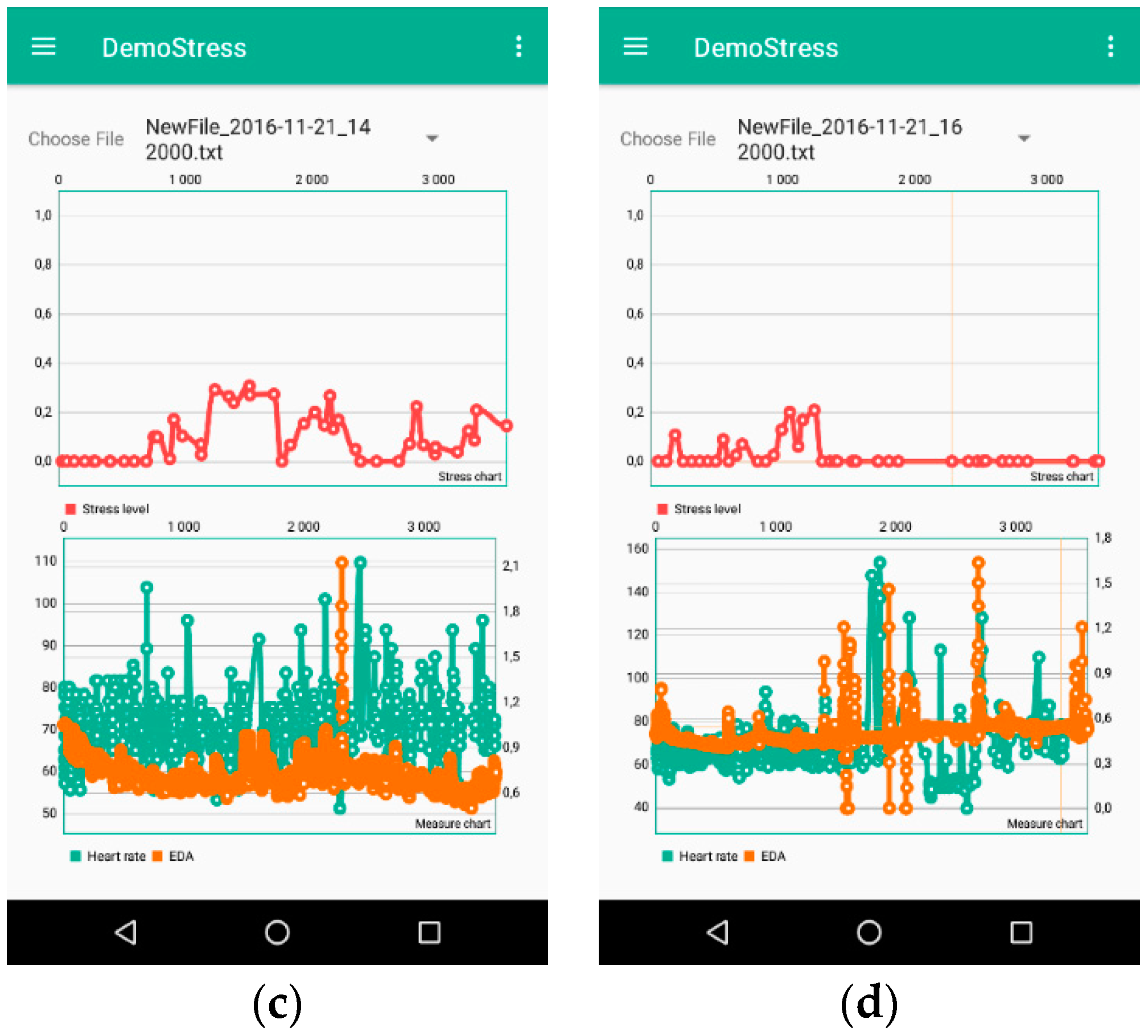
The test phase took place two months after the learning acquisition, during a travel between the cities of Grenoble (France) and Brussels (Belgium) where our participant had to attend another meeting with partners. Throughout the journey, a homemade smartphone application continuously recorded peripheral sensor data from the same smart wristband that was used for model calibration. In the meantime, it used the personalized stress model to timely estimate and record participant’s stress levels, with a 60-s time resolution Figure 1 shows four screenshots of algorithm’s outputs on as many 1h time periods, displayed by means of the application user interface. For the sake of clarity, model outputs were clipped so that stress levels displayed on the GUI are contained in the [0 1] range, and the missing data were interpolated.
On each picture, the top chart shows the estimated stress levels, and the bottom chart shows the two main signals of interest: heart rate and the skin conductance level. During the time interval displayed in Figure 1a, an unfortunate setback happened at the working place a few hours before the shuttle departure: participant witnessed a server crash that might have compromised the main goal of the journey he was about to undertake. This resulted in a large peak of stress, which has been successfully recovered by the algorithm: it can be noticed in the middle of the top chart. The three other screenshots in Figure 1b–d are about the trip itself. The time interval considered in picture b takes place in the airport shuttle (total travel time: 83 min, mean stress reported by the user: 3/10). Picture c corresponds to the 1st h by train (out of four), when the participant was working on his desktop (total working time: 2 h, mean stress reported by the user: 2/10). Figure 1d corresponds to his 3rd hour in the same train, just after the participant had stopped working (total time remaining still: 2 h, mean stress reported by the user: 1/10).
Finally, on the bottom charts of Figure 1, artefacts can be observed in the two displayed signals (heart rate and the skin conductance level). However, model outputs remained stable. This could be explained by some redundancy of information within the set of features and available signals: at a given time, the model was still able to assess a stress level in spite of isolated artefacts.
2.2.2. Estimation Performances
For the last three (non-stressful) conditions described above, the RMSE from participant’s self-rated stress level was computed, along with the proportion of correctly classified 60 s time windows. The results are shown in Table 2 below. The second column gives the number of instances per period. Stress was not estimated when the heart rate data was not available enough for feature extraction (see Section 4): this explains why the number of time windows does not sum up to the total duration of each condition. The third column shows RMSEs of raw model outputs for each period. The fourth column shows RMSEs for the data displayed in Figure 1, i.e., clipped between 0 and 1. The last column displays the classification rate (actually a true negative rate) for each condition, and its expected error rate. The last line displays the mean value and error for each of these columns.
One may notice that classification performance for the relaxed condition (i.e., “Train II”) reaches the maximum value. This period also shows the greatest performances in RMSE. Classification rates remain high in all three conditions, the greatest false positive rate (7.4%) being reached in the most active condition (‘Train I”).
3. Discussion
A lot of improvements are still to be made in the physiological stress model reported in this paper. As further stated in Section 4, we used a simple linear model for regression and classification, and purposely did not perform feature selection. Such an optimization is our next step in developing a human stress model, but this also requires collecting data from a larger set of participants, and to get more information about their psychological feelings and environmental factors that may influence the recorded physiological signals. In that perspective, the feature set could be optimized both by enrichment (considering other kinds of signal properties) and reduction (performing efficient feature selection). Additionally, more complex models should be tested, which might provide more accurate and robust estimations.
Still, our approach brought up some interesting results. For instance, the two train examples in Figure 1 illustrate the influence of ambulatory conditions on model performances: as soon as the participant stopped working on his laptop, the stress level assessed by our model decreased, along with RMSEs on the reported stress levels; and all samples were correctly labelled as no-stress data. This phenomenon could be timely monitored as shown in Figure 1c,d. Even though the variability in physiological signals is intrinsically taken into account by our model through the feature set, notably with features based on standard deviation, real-life conditions will still decrease its accuracy. What is more, it should be noted that participant’s stress levels unlikely remained the same all the time during each condition, as assumed in this preliminary study—in our approach, we considered as the ground truth the mean stress level reported by the user over a given period.
Regarding the matter of ground truth, determining which kinds of events are the most suitable to train a stress detection model is not a trivial question. In an end-user setting, soliciting user intervention as little as possible is a key issue: to calibrate a reliable stress model, an efficient trade-off has to be found between user acceptance and algorithm’s requirements, regarding information collection on affective states and environmental factors. In our experimental design, a compromise had thus to be brought up between, on the one hand: full awareness on environmental factors and participant’s feelings, and on the other hand: some coarse ground truth, related to specific events. We hence designed our grey-box model on the grounds of three stressful and one control conditions (the last one being non-stressful but still active), delineated in retrospect by the user himself.
The three self-reported periods of moderate-to-high stress occurred in different circumstances. Varying participant’s environment, mental or physical activity during the stress condition was a prerequisite to the construction of a general model, whose accuracy would extend to any new stressful situation. Furthermore, adding an event that was not related to the trip itself (e.g., giving a speech during a meeting) allows assessing the ubiquitous nature of the psychological state that is quantified—given that stress is not specific to travelling. This could be seen during the cross-validation with Trial N°3 (Table 1), where the “speech” event was used as a validation dataset: the model, trained on the other stressful episodes taken from the journey, successfully applied to the oral presentation period, with similar RMSEs for learning and validation steps.
However, a main limitation of this study lies in the small number of available events for the no-stress condition: this likely explains the perfect classification rate shown in Table 1. Indeed, unusual environmental factors might have strongly affected one or more peripheral measurements during the no-stress period, which would have led to an overfitting effect. In this case, our algorithm should focus more on detecting these influential factors rather than user’s psychological stress. Such a hypothesis may be argued by the higher RMSEs obtained during the test phase (Table 2) than during the validation steps (Table 1): on new no-stress events, the model has shown up less accurate with respect to participant’s reported stress levels. However, our algorithm remained efficient in classifying all three test events as actually non-stressful episodes.
In a nutshell, we succeeded in recovering the stressful (or non-stressful) nature of episodes that took place during a medium-length trip, using a linear combination of statistical features extracted from the raw physiological data. This model has been implemented in a smartphone application, allowing for real-time estimation of user’s stress levels using a minimally invasive setting: a smart wristband connected with user’s own phone. Our purpose here was to present preliminary results and to highlight the potential of such a tool for the future of mass transit. In the Bonvoyage H2020 framework for instance, the digital platform will automatically infer a user profile based on the timely assessed stress in different transport modes during previous travels or commutes. This profiling will be used to propose tailored solutions to users in order to improve their on-board experience. Real-time monitoring of passenger’s stress also aims at proposing an on-trip assistance to deal with excessive stress during any travel, by suggesting an alternative trip solution. In a more large-scale use, statistical data could be drawn by crowdsourcing on passengers’ feelings about transportation means, which would bring service providers closer from consumers’ wellbeing. At the individual level, this can be an efficient way to raise people’s awareness over their own living standards.
4. Materials and Methods
The next paragraphs describe in further details the materials and methods mentioned in Section 2.
4.1. Ethics Approval, Consent, Availability of Data
The experiment described in this article is part of an experimental campaign approved by the Ethics Committee in Non-Interventional Research (CERNI) related to COMUE Université Grenoble-Alpes, and in accordance with the Declaration of Helsinki. Following a standard inclusion procedure, the participant provided written consent to participate, and agreement—subject to full anonymity—for publication of results based on collected psychological and physiological data. However, the raw data acquired throughout this experiment will not be made available for public use, in accordance with a confidentiality agreement between the participant and the research team.
4.2. Physiological Recording
The wearable sensor Empatica™ E4 wristband was used to record three different physiological signals: blood volume pulse (BVP), skin conductance (SC) and skin temperature; and 3-axis accelerometer data. This device can be used in two separate ways: either in storage mode (data is stored in the wristband’s local memory), or in streaming mode (transmission by Bluetooth® connection to a suitable smartphone application). The storage mode has been used during the learning phase, the streaming mode during the test phase. The BVP signal is an Empatica’s proprietary version of pulse oximetry: by measuring the oxygen saturation in blood vessels at the surface of the skin, it allows an indirect measure of heart rate. In Empatica™ E4, BVP is recorded at 64 Hz, SC at 4 Hz, 3-axis acceleration at 32 Hz and skin temperature at 4 Hz. The wristband automatically infers interbeat intervals (IBIs) when data’s quality is high enough. Its battery and memory units are sufficient to enable more than one day of continuous recording. The device is also equipped with a trigger button which allows the participant to mark some significant events, and the experimenter to locate them easily in time.
4.3. Preliminary Signal Processing
The SC signal has been processed in two different ways. The first one is a slight signal smoothing, performed by applying a 2nd order low-pass Butterworth filter with a cut-off frequency set to 0.2 Hz. This allows removing peaky artefacts from the signal, such as pressure waves, or zeros caused by one-time contact losses between electrodes and the skin—and nonetheless, to preserve the main skin conductance responses (SCRs). The second processing is a harder signal smoothing, also performed by a 2nd order low-pass Butterworth filter, with a cut-off frequency set to 0.05 Hz: the remaining information corresponds to the skin conductance level (SCL). SCL is the main tonic component of SC: it is related to the current physical properties of the skin and to individual’s general arousal level. SCRs consist in punctual rises in the skin conductance that are potentially triggered by emotional events, with a progressive return to SCL; they represent the main phasic component of SC. They are the part of interest in the first processed signal, which includes both the tonic and phasic information.
The IBI signal is derived from BVP by an Empatica™ proprietary algorithm that performs a real-time recognition on the BVP waves. It is not regularly sampled, and the poor signal-to-noise ratio brought on BVP by ambulatory conditions makes wave recognition difficult, generating sometimes a sparse IBI signal. The HR signal is inversely proportional to the IBI.
Only the Euclidian norm was considered for the 3-axis accelerometer data. No post-processing was applied to the skin temperature signal: raw data were used.
4.4. Feature Computation
Following this first step, 24 statistical features were computed from the processed signals, which are displayed in Table 3. Each one of them has been calculated over successive 60-s time windows, with no overlapping. They have been selected on the basis of previous work on experimental databases [12,13], and for their suitability for real-time implementation.
Regarding the electrodermal activity, with respect to the four different features computed from the local maxima in the SC curve (SCRs), previous filtering allows setting minimal constraints on the detection parameters, without time delay between two peaks and with a threshold prominence set to 10−3 μS. For a given peak, the prominence is defined as its height, relatively to the lowest point located between this peak and the nearest higher peak (for more detailed information see [14]). The peak width is defined as the number of samples, within this peak, which the ordinate exceeds its half prominence.
Regarding cardiac activity, given that the IBI signal is not steadily sampled, the frequency domain features have been derived from its Lomb-Scargle power spectral density estimate on each time window. When no IBI data could be found, the time window was discarded from the whole analysis. After feature extraction, the cleaned feature matrix included 84 non-stress and 137 stress examples, which represent 78.4% of the initial database.
Since real-time computations were intended, no artefact rejection was performed on the remaining dataset. Together with the expected poor signal-to-noise ratio in ambulatory conditions, this motivated the use of the whole feature set to fully take advantage of information content from all the recorded signals.
4.5. Linear Regression Model
The final stress model has been designed as a weighted sum on each of the previous statistical features. The predicted stress level s over one time window t is expressed in Equation (3), where F is the number of features, each of which fk is associated with a weight βk that quantifies its linear relationship with s.
To estimate the full weight vector β, a linear regression has been performed using the least-squares method on the feature matrix extracted from a learning database: the one recorded during participant’s first trip.
4.6. From Learning to Test Phase
The previous model is the one described all along Section 3. Following the validation stage, the results of which are displayed in Table 1, the final β weight vector was estimated using the whole learning database. All the required steps for stress estimation (first processing, feature computation and combination within the linear model) were then implemented in a home-made Android application, able to communicate with the E4 wristband in streaming mode. The overall framework (wristband-smartphone-application) was able to record the same user’s physiological signals and estimate his stress levels every minute in real time. This setting was put on test during the journey from Grenoble to Brussels. Model outputs are those displayed in Figure 1.
Author Contributions
Conceptualization, C.G. and E.L.; Methodology, O.S. and G.V.; Software, S.O. and A.V.; Investigation, E.L.; Data curation, S.O. and O.S.; Writing—Original draft preparation, G.V.; Writing—Review and editing, C.G., E.L., A.C. and G.V.; Supervision, S.C., A.C. and C.G.; Funding acquisition, C.G. and E.L.
Funding
This project has received funding from the European Union’s Horizon 2020 research and innovation program under grant agreement No 635867.
Conflicts of Interest
All authors declare having neither financial nor non-financial interest in publishing the previous results or citing any research material. The funders had no role in the design of the study; in the collection, analysis, or interpretation of the data; in the writing of the manuscript, or in the decision to publish the results.
References
- McEwen, B.S. The neurobiology of stress: from serendipity to clinical relevance. Brain Res. 2000, 886, 172–189. [Google Scholar] [CrossRef]
- Lazarus, R.S.; Folkman, S. Transactional theory and research on emotions and coping. Eur. J. Personal. 1987, 1, 141–169. [Google Scholar] [CrossRef]
- European Foundation for the Improvement of Living and Working Conditions (Ed.) The Journey from Home to the Workplace: The Impact on the Safety and Health of the Commuters/workers: Consolidated Report; European Foundation for the Improvement of Living and Working Conditions: Dublin, Ireland, 1984. [Google Scholar]
- Legrain, A.; Eluru, N.; El-Geneidy, A.M. Am stressed, must travel: The relationship between mode choice and commuting stress. Transp. Res. Part F Traffic Psychol. Behav. 2015, 34, 141–151. [Google Scholar] [CrossRef]
- Cox, T.; Houdmont, J.; Griffiths, A. Rail passenger crowding, stress, health and safety in Britain. Transp. Res. Part Policy Pract. 2006, 40, 244–258. [Google Scholar] [CrossRef] [Green Version]
- Wener, R.E.; Evans, G.W. Comparing stress of car and train commuters. Transp. Res. Part F Traffic Psychol. Behav. 2011, 14, 111–116. [Google Scholar] [CrossRef]
- Greene, S.; Thapliyal, H.; Caban-Holt, A. A Survey of Affective Computing for Stress Detection: Evaluating technologies in stress detection for better health. IEEE Consum. Electron. Mag. 2016, 5, 44–56. [Google Scholar] [CrossRef]
- Kim, H.-G.; Cheon, E.-J.; Bai, D.-S.; Lee, Y.H.; Koo, B.-H. Stress and Heart Rate Variability: A Meta-Analysis and Review of the Literature. Psychiatry Invest. 2018, 15, 235–245. [Google Scholar] [CrossRef] [PubMed] [Green Version]
- Boucsein, W. Electrodermal Activity; Springer Science & Business Media: Berlin/Heidelberg, Germany, 2012; ISBN 9781461411260. [Google Scholar]
- Healey, J.A.; Picard, R.W. Detecting stress during real-world driving tasks using physiological sensors. IEEE Trans. Intell. Transp. Syst. 2005, 6, 156–166. [Google Scholar] [CrossRef]
- Hovsepian, K.; al’Absi, M.; Ertin, E.; Kamarck, T.; Nakajima, M.; Kumar, S. Stress: Towards a Gold Standard for Continuous Stress Assessment in the Mobile Environment. Proc. ACM Int. Conf. Ubiquitous Comput. UbiComp Conf. 2015, 2015, 493–504. [Google Scholar]
- Ollander, S.; Godin, C.; Campagne, A.; Charbonnier, S. A comparison of wearable and stationary sensors for stress detection. In Proceedings of the 2016 IEEE International Conference on Systems, Man, and Cybernetics (SMC), Budapest, Hungary, 9–12 October 2016; pp. 004362–004366. [Google Scholar]
- Ollander, S.; Godin, C.; Charbonnier, S.; Campagne, A. Feature and Sensor Selection for Detection of Driver Stress; SCITEPRESS—Science and Technology Publications: Setúbal, Portugal, 2016; pp. 115–122. [Google Scholar]
- MathWorks, Inc. Available online: https://www.mathworks.com/help/signal/ug/prominence.html (accessed on 25 April 2019).
Figure 1.
Screenshots of the smartphone application user interface, taken the during test phase (travel from Grenoble to Brussels). On each screenshot, top chart shows the timely estimated stress levels (in red). Bottom chart displays the corresponding raw physiological signals: heart rate [bpm] in green, and skin conductance [μS] in orange. (a) First setback (7:20 to 8:20); (b) Airport shuttle (12:20 to 13:20); (c) Work in train (14:20 to 15:20); (d) Leisure in train (16:20 to 17:20).


Table 1.
Performances for each trial during cross-validation.
| Trial | -----------On the Training Set----------- | ----------On the Validation Set---------- | ||||
|---|---|---|---|---|---|---|
| N° | No. Ex. Ns/S | RMSE | Cr % | No. Ex. Ns/S | RMSE | Cr % |
| 1 | 56/74 | 0.066 ± 0.009 | 100 ± 0 | 28/63 | 0.090 ± 0.015 | 100 ± 0 |
| 2 | 56/72 | 0.048 ± 0.007 | 100 ± 0 | 28/65 | 0.143 ± 0.024 | 100 ± 0 |
| 3 | 56/128 | 0.070 ± 0.008 | 100 ± 0 | 28/9 | 0.086 ± 0.025 | 100 ± 0 |
| Mean | - | 0.061 ± 0.008 | 100 ± 0 | - | 0.106 ± 0.021 | 100 ± 0 |
Table 2.
Performances for each transport mode during the test phase.
| Mode | No. Ex. | RMSE (Raw Output) | RMSE (Clipped Output) | Cr % |
|---|---|---|---|---|
| Shuttle | 68 | 0.202 ± 0.041 | 0.189 ± 0.039 | 97.1 ± 4.0 |
| Train I | 95 | 0.189 ± 0.031 | 0.154 ± 0.026 | 92.6 ± 5.3 |
| Train II | 83 | 0.171 ± 0.031 | 0.094 ± 0.017 | 100 ± 0 |
| Mean | - | 0.187 ± 0.035 | 0.146 ± 0.027 | 96.5 ± 3.2 |
Table 3.
Feature set.
| Description |
|---|
| Mean interbeat interval (IBI) |
| IBI standard deviation |
| Root mean square of the successive differences in IBI |
| Mean heart rate (HR) |
| HR standard deviation |
| Ratio of the HR mean over standard deviation |
| Root mean square of the successive differences in HR |
| Total power in the IBI signal |
| IBI signal power in the Low Frequency (LF) band [0.04 Hz 0.15 Hz] |
| Previous value normalized by the total power in IBI |
| IBI signal power in the High Frequency (HF) band [0.15 Hz 0.5 Hz] |
| Previous value normalized by the total power |
| Ratio of the previous LF and HF frequency components |
| Mean of the SCL signal |
| Mean of the 1st temporal derivative on the SCL signal |
| Standard deviation of the SC signal |
| Number of local maxima (SCRs) on the SC curve |
| Mean prominence of the SCRs |
| Mean width of the SCRs |
| Sum of all SCRs’ width-prominence products |
| Mean Skin Temperature |
| Mean of the 1st temporal derivative of the Skin Temperature |
| Total power of the Acceleration norm |
| Mean absolute deviation of Acceleration norm |
© 2019 by the authors. Licensee MDPI, Basel, Switzerland. This article is an open access article distributed under the terms and conditions of the Creative Commons Attribution (CC BY) license (http://creativecommons.org/licenses/by/4.0/).
Share and Cite
MDPI and ACS Style
Vila, G.; Godin, C.; Sakri, O.; Labyt, E.; Vidal, A.; Charbonnier, S.; Ollander, S.; Campagne, A. Real-Time Monitoring of Passenger’s Psychological Stress. Future Internet 2019, 11, 102. https://doi.org/10.3390/fi11050102
AMA Style
Vila G, Godin C, Sakri O, Labyt E, Vidal A, Charbonnier S, Ollander S, Campagne A. Real-Time Monitoring of Passenger’s Psychological Stress. Future Internet. 2019; 11(5):102. https://doi.org/10.3390/fi11050102
Chicago/Turabian StyleVila, Gaël, Christelle Godin, Oumayma Sakri, Etienne Labyt, Audrey Vidal, Sylvie Charbonnier, Simon Ollander, and Aurélie Campagne. 2019. "Real-Time Monitoring of Passenger’s Psychological Stress" Future Internet 11, no. 5: 102. https://doi.org/10.3390/fi11050102
Note that from the first issue of 2016, this journal uses article numbers instead of page numbers. See further details here.