Tax Fraud Detection through Neural Networks: An Application Using a Sample of Personal Income Taxpayers

Abstract

The goal of the present research is to contribute to the detection of tax fraud concerning personal income tax returns (IRPF, in Spanish) filed in Spain, through the use of Machine Learning advanced predictive tools, by applying Multilayer Perceptron neural network (MLP) models. The possibilities springing from these techniques have been applied to a broad range of personal income return data supplied by the Institute of Fiscal Studies (IEF). The use of the neural networks enabled taxpayer segmentation as well as calculation of the probability concerning an individual taxpayer’s propensity to attempt to evade taxes. The results showed that the selected model has an efficiency rate of 84.3%, implying an improvement in relation to other models utilized in tax fraud detection. The proposal can be generalized to quantify an individual’s propensity to commit fraud with regards to other kinds of taxes. These models will support tax offices to help them arrive at the best decisions regarding action plans to combat tax fraud.

1. Introduction

The quantification and detection of tax fraud is a top priority amongst the most important goals of tax offices in several countries. The estimates regarding tax fraud at the international level reveal that Spain is one of the developed countries with a high level of tax fraud, exceeding 20% of GDP [1,2,3]. Despite the measures implemented to curtail this, to date, there has been no reduction with respect to the trend [4,5].

In view of the significance of the problems resulting from tax fraud, and bearing in mind efficiency, equity, and the capacity to procure money, it is evident that improving the efficacy of measures to reduce tax fraud is high on the list of tax offices priorities. Designing control systems for detecting and fining people who do not fully meet their tax obligations could be crucial to lessening the problem. Making fraud detection easier in addition to achieving higher efficacy with respect to inspections could result in greater levels of tax compliance. In this sense, although empirical studies have not corroborated an increase in tax inspections leading to a reduction in the number of tax fraud cases [6,7], the availability of tools to streamline and heighten efficiency, where checks are concerned, would be of help in the battle to curtail fraud. Also, the development of new technologies and the considerable increase in information available for fiscal purposes (big data) provides an opportunity to reinforce the work done by tax offices [8,9,10].

Accordingly, this paper attempts to make a contribution through research conducted on the application of Neural Network models to income tax returns samples provided by the Spanish Institute of Fiscal Studies, with a view to facilitating the detection of taxpayers who evade tax by quantifying an individual taxpayer’s tendency to commit fraud. With this goal in mind, use was made of Machine Learning advanced predictive tools for supervised learning, specifically of the neural networks model.

A very significant added value of this study is the utilization of databases pertaining to official administrative sources. This means that there are no problems arising from missing data, nor other data flaws. The information used is the official data from the Spanish Revenue Office, (https://www.agenciatributaria.es/) implying their validity, tax analysis, and taxpayer inspection is based on the said data [11]. In particular, the IRPF sample utilized in this study is the main instrument for fiscal analysis.

Lastly, the methodology resorted to in this paper can be generalized to quantify each taxpayer’s propensity to commit any other kind of tax fraud. The availability of huge data sets containing information on each taxation concept allows the utilization of a generic methodology to widen possibilities with regards to quantitative analysis and also to take advantage of the new services provided by big data, data mining, and Machine Learning techniques.

The structure of this article is as follows: The second section presents the background and describes the methodological approach applied in this study. The third section deals with the estimation and adjustment strategy. Additionally, in the same section, the sensitivity of the model concerning the entire training and sample is explored. The last section consists of a brief conclusion, in addition to detailing future research possibilities arising from the results obtained.

2. Background and Methodological Framework

In recent years, artificial intelligence has become a tool which permits the handling of huge databases as well as the use of algorithms which, although complex in structure, provide results which may be interpreted easily. This framework offers the possibility of detecting and checking fiscal fraud which is an area that has aroused the interest of researchers, and generated concern for public administrative offices. In this paper, the proposal put forward focuses not only on the utilization of neural networks for detecting fiscal fraud as regards taxpayers in Spain, but also on contributing to precise fraud profiling to facilitate tax inspections. From the literature, data mining techniques present several possibilities for data processing aimed at fraud analysis [12].

Neural network models normally outperform other predictive linear and non-linear models where perfection and predictive capacity are concerned [13,14,15]. From the quantitative perspective, they often consist of optimum combinations which permit better prediction and more accurate estimations than occurs with other types of models. The neural network facilitates classification of each tax filer as fraudulent or not fraudulent, and furthermore, it reveals a taxpayer’s likelihood to be fraudulent. In other words, it does not only classify individuals as prone to fraud or not, but also computes each filer’s probability to commit fraud. Hence, tax filers are classified according to their propensity to commit fraud.

Attaining the above-mentioned goal comes with a price due to software availability (suitable software for these techniques is not common), computation capacity (network algorithms are rather complicated and require adequate hardware for convergence), and methodological control (Machine Learning techniques are not trivial concerning methodology). To meet the objectives of this study, IBM software and hardware were used (www.ibm.es) to achieve the algorithm convergence of neural networks applied to millions of data and hundreds of variables. On the other hand, as any graphic representation which involves millions of points cannot be done without infrastructure which is appropriate for huge amounts of data, the same programming has been utilized.

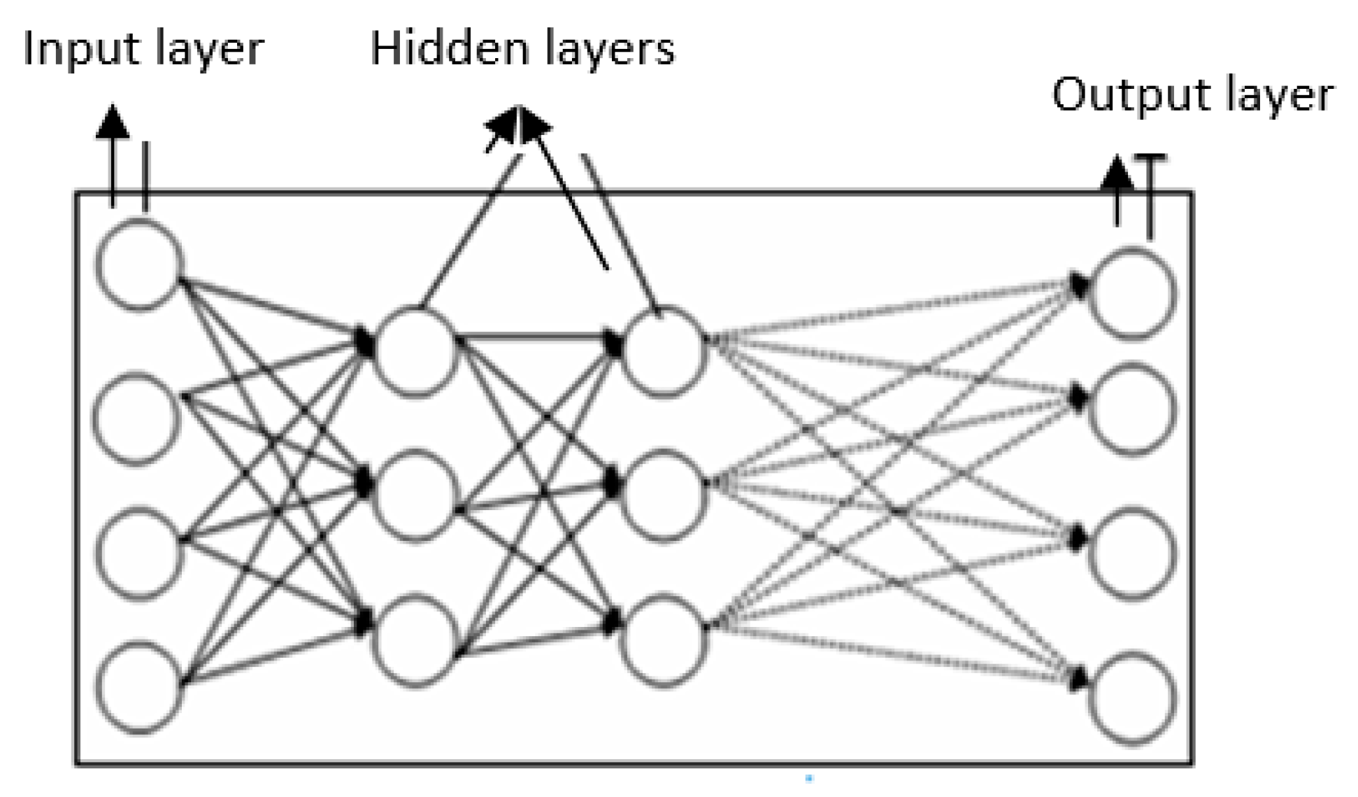
We can define an artificial neural network as an intelligent system capable not only of learning, but also of generalizing. A neural network is made up of processing units referred to as neurons and nodes. The nodes are organized in groups called “layers”. Generally, there are three types of layers: An input layer, one or several hidden layers, and an output layer. Connections are established between the adjacent nodes of each layer. The input layer, whereby the data is presented to the network, is made up of input nodes which receive the information directly from outside. The output layer represents the response of the network to the inputs received by transferring the information out. The hidden or intermediate layers, located in between the input and output layers, process the information and are the only layers which have no connection to the outside.

The most commonly found network structure is a type of network which is fed forwards or referred to as a feedforward network, since the connections established between neurons move in one direction only according to the following order: The input layer, hidden layer(s), and the output layer. For example, Figure 1 depicts a feedforward network with two hidden layers.

Nevertheless, it is also possible to find feedback networks which have connections moving backwards, that is, from the nodes to the processing elements of previous layers, as well as recurrent networks with connections between neurons in the same layers, as well as a connection between the node and itself. Figure 2 illustrates a network model where the different types of mentioned connections can be found moving forwards, backwards, and also in a recurrent pattern, resulting in a fully interconnected network.

A fully interconnected neural network occurs when the nodes in each layer are connected to the nodes in the next layer. The sole mission of the input layer is to distribute the information presented to the neural network for processing in the next layer. The nodes in the hidden layers and in the output layer process the signals by applying processing factors, known as synaptic weights. Each layer has an additional node referred to as bias, which adds an additional term to the output from all the nodes found in the layer. All inputs in a node are weighted, combined, and processed through a function called a transfer function or activation function, which controls the output flow from that node to enable connection with all the nodes in the next layer. The transfer function serves to normalize the output. The connections between processing elements are linked to a connection weight or force W, which determines the quantitative effect certain elements have on others.

Specifically, the transformation process for the inputs and outputs in a feedforward artificial neural network with r inputs, a sole hidden layer, composed of q processing elements and an output unit can be summarized in the following formulation of the network output function for the following model (1) and in Figure 3:

$$Y=\widehat{f}(x,W)=F\left({\beta }_0+{\displaystyle \sum _{j=1}^q{\beta }_{j}G(x^{\prime }{\gamma }_j)}\right)$$

(1)

where:

• $x=(1,x_1,x_2,\dots ,x_r{)}^{\prime }$ are the network inputs (independent variables), where 1 corresponds to the bias of a traditional model.
• ${\gamma }_j=({\gamma }_{j0},{\gamma }_{j1},\dots ,{\gamma }_{ji},\dots ,{\gamma }_{jr}{)}^{\prime }\in {\Re }^{r+1}$ are the weights of the inputs layer neurons to those of the intermediate or hidden layer.
• ${\beta }_j,j=0,\dots ,q$, represents the connection force of the hidden units to those of pertaining to output ($j=0$ indexes the bias unit) and q is the number of intermediate units, that is, the number of hidden layer nodes.
• W is a vector which includes all the synaptic weights of the network, ${\gamma }_j$ and ${\beta }_j$, or connections pattern.
• Y = $\widehat{f}(x,W)$ is the network output (in our case, it refers to fraud probability)
• F: ℜ → ℜ is the unit activation function and output while G: ℜ → ℜ corresponds to the intermediate neurons activation function. Selection of both was considered optimum, in accordance with the software utilized (It is normal to use the sigmoid or logistic function G(a) = 1/(1 + exp(-a)), which produces a smooth sigmoid response. Notwithstanding, it is possible to use the hyperbolic tangent function. In the expression $\widehat{f}(x,W)$ if we consider that $a=x^{\prime }{\gamma }_j$, we find that G($x^{\prime }{\gamma }_j$) tallies with the binary logit model).

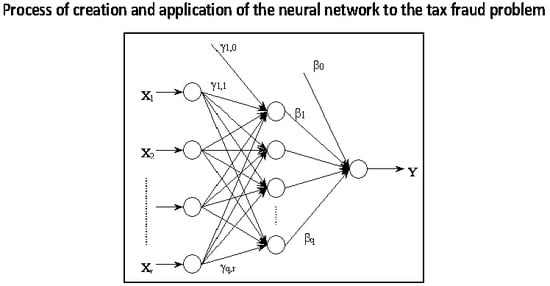
As to the creation and application of a neural network to a specific problem, the following steps are shown in Figure 4:

The neural network model we are going to apply in this study is the supervised learning model based on the multilayer perceptron. There are other neural network models such as the Radial Basis Function (RBF), which is also interesting for this kind of analysis. Accordingly, it was utilized to compare its efficiency against that of the model presented, confirming that the multilayer perceptron provides the best results. The results obtained with the Radial Basis Function model are available upon request), given that it presents an output pattern or dependent variable which allows for contrasting and correcting data. Due to this, it is a technique used for classification as well as for prediction, for market segmentation, the positioning of products, forecasting demand, evaluation of credit files or analysis of stock exchange value, in addition to a countless number of other applications. Specifically, the multilayer perceptron stems from back-propagation error learning. It is the most frequently utilized algorithm, and besides, it mostly makes use of the backpropagation algorithm, the conjugate gradient descent, or the Levenberg-Marquardt algorithm. The advantages of the multilayer perceptron over other procedures can be attributed to the fact that all layers have the same linear structure, thereby rendering it more efficient.

3. Tax Fraud Modeling with Neural Networks

3.1. Data Matrix: IRPF Sample Provided by the IEF

For the application presented here, the data consists of the sample of Personal Income Tax returns (in Spanish, IRPF) filed in 2014 and which was obtained from the Institute of Fiscal Studies (in Spanish IEF). The sample consists of highly accurate data which is, moreover, characterized by an absence of problems related to infra-representation or the habitual lack in survey responses. With respect to the demographic scope, personal income tax (IRPF) returns filed in the previously mentioned year were used. The geographical area encompasses the Common Tax System Territory (excluding the Basque Country and Navarra). The period in question refers to 2014 fiscal year, bearing in mind that the samples had been compiled and published on a yearly basis, starting from 2002. Details pertaining to the methodology and the sample design, as well as the advantages and drawbacks can be found in recent papers [11,16].

3.2. Conceptualization of the Model: Application of the Tax Fraud Detection Model to Income Tax Returns

To build the Multilayer Perceptron supervised learning neural network model, the dependent variable used (single network output variable) is a dichotomous variable which takes a value of 1 if the individual in question commits fraud and the value zero cero if no fraud is detected on the part of the individual (mark variable). The independent variables (network input variables) constitute the most important items regarding personal income tax.

The purpose of the neural network model is to predict the probability any individual has to evade tax or otherwise, in accordance with the values declared in the variables included in Income Tax Form 100, available on the Spanish tax office website https://www.agenciatributaria.gob.es/AEAT.sede/procedimientoini/G229.shtml.

Taking this to be our point of departure, our ensuing analysis will enable us to draw up fraud profiles which could be of help during future tax inspections.

In this study, the independent variables used for the neural network model are considered to be the most important economic entries in relation to personal income taxation, as they are the concepts usually targeted by taxpayers attempting to evade tax. The entries in question include practically all the others as sum totals.

The following

Table 1. Independent variables of the neural network model.

Concept	Box
Earnings
Gross work income (monetary)	par1
Net work income	par15
Capital gains gross income	par29 + par45
Capital gains net income	par31 + par47
Deductible net capital gains	par35 + par50
Gross property income	par70
Capital gains net income	par75
Deductible net property income	par79 = par85
Total deduction net income from economic activities under direct evaluation scheme	par140
Net earnings from economic activities under objective evaluation scheme (except agricultural, livestock forestry activities).	Par170
Net earnings from crop, livestock and forestry activities under objective evaluation scheme	Par197
Capital gains and losses positive net balance	par450 + par457

and

Table 2. Income tax minimum and base variables.

Concept	Box
Minimums and Bases
General taxable base	par455
Savings taxable base	par465
Minimum personal and family, part of general applied	par680
Minimum personal and family, part of savings applied	par681
Liquidable general base levy on	par620
Taxable savings base on saving	par630
Quotas
Central government tax	par698
Regional government tax	par699
Central government net tax	par720
Regional government net tax	par721
Self-assessment tax liability	par741
Tax payable	par755
Tax return balance	Par760

present the mentioned entries, which have been grouped in accordance with the different tax concepts: Independent variables, income tax minimum, and base variables:

Reductions applied to the taxable base will also be taken into account:

We consider the total reduction applied to the taxable base to be the following variable:

$$\mathrm{Taxable}\mathrm{base}\mathrm{rebates}=par470+par500+par505+par530+par560+par585+par600$$

Another significant group of tax variables correspond to deductions on account of housing, gifts, autonomous regional government deductions, investment boosting incentives, and other deductions.

The applicable deductions have been grouped into variables as follows:

$$\begin{array}{l}\mathrm{Housing}\mathrm{deductions}=par700+par701+par716\\ \mathrm{Gift}\mathrm{deductions}=par704+par705\\ \mathrm{Other}\mathrm{deductions}=par702+par703+par712+par713+par714+par715\\ \mathrm{Regional}\mathrm{government}\mathrm{deductions}=par717\\ \mathrm{Investment}\mathrm{incentive}\mathrm{deductions}=par706+par707\end{array}$$

Also taken into consideration are the total deductible expenses related to income accrued from work and from capital gains (par14 + par30 + par46), as shown in the following variable:

$$\mathrm{Total}\mathrm{deductible}\mathrm{expenses}=par14+par30+par46$$

As to the dependent variable, due to the confidential nature of taxpayer data and the attendant legal requirements—which have been scrupulously adhered to throughout our research—the sample data on individual fraudulent and non-fraudulent tax filers follow the actual pattern without coinciding exactly with the concrete data. Moreover, the database used was completely anonymized. In practice, the fraudulent taxpayers would be those people in the sample that an inspection had determined, without a shadow of a doubt, to have been fraudulent.

Nevertheless, this research has been conducted independently of the year the data stems from since the goal is to find a methodology to obtain a tax fraud prediction function to enable quantification of income taxpayers’ propensity to evade tax.

3.3. Dimension Adjustment: Reduction of the Dimension According to the Main Components

Our model features a series of quantitative independent variables, correlated with each other, that would trigger a multicollinearity problem in any model to be estimated. Consequently, it is imperative to reduce said variables to their uncorrelated main components. Adjusting the model to its components would eliminate the multicollinearity, in addition to reducing the impact of atypical values, and also bring about variable normality. Accordingly, after component adjustment, the model properties would be considered as optimum.

In this case, the reduction can be taken to be legitimate because the matrix determinant, relative to the initial variables correlation, is practically null. Moreover, the commonalities of the variables are high, with many of them close to the unit. As a result of the analysis carried out, we have obtained 11 Ci main components (factors), which account for close to 85% of the initial variability of the data, thereby securing a satisfactory reduction. In more specific terms, the components account for 84.882% of the variability, after a VARIMAX rotation.

Analysis of the factorial matrix revealed that the first component –C1– comprises the first 17 variables, which include earnings, bases, and quotas. The second component –C2– includes four variables related to the asset balances, tax and result of the filed tax return. The third component –C3– encompasses 5 variables related to capital gains tax and savings base tax. The fourth component –C4– contains 4 variables relative to fixed capital assets. Component C5 comprises 2 variables, namely regional government, and gift deductions. Component C6 comprises three variables pertaining to housing, and minimum personal and family deductions. Component C7 involves a single variable dealing with economic activities. Component C8 comprehends two variables related to taxable base and pension scheme deductions. Component C9 contains 3 variables pertinent to total deductible expenses and investment incentives deductions. Component C10 is a single variable relevant to positive net balance, on account of capital gains and losses. Lastly, component C11 comprises two variables pertaining to the net return regarding agrarian modules and other deductions. Hence, the factorial matrix makes it possible to express each of the 11 main components as a linear combination of the comprising initial variables and in a disjoint manner.

The main components obtained are the input variables of the neural network model (independent variables). The output variable corresponds to the dichotomous mark variable, where value 1 indicates fraud, while zero value denotes the absence of fraud.

3.3.1. Multilayer Perceptron Network Model Estimation and Diagnosis Phase

For this research, feedforward artificial neural networks have been utilized, with r inputs (the most significant variables or income tax return items which are liable to be targeted for fiscal fraud), a sole hidden layer composed of processing elements q, and an output unit (fraud variable for indicating whether an individual has avoided tax or not). The network will make tax fraud modeling possible in the case of personal income tax returns and also permit assessment of an individual’s propensity to fraudulent practices.

Estimation of the Multilayer Perceptron model, as depicted in model (1), was carried out with the 11 main components obtained in the previous section as the input variables, while the mark variable served as the output variable.

There are several advantages to using the main components as input variables in model (1). Firstly, the effect of the atypical values is eliminated since the component values have a far lower range than the initial variables. Given that the components are linear combinations of the initial variables, the effects of the atypical values are reduced. Secondly, data confidentiality increases since it is very difficult to identify individuals from the component values. Thirdly, multicollinearity problems in the model are eliminated because the components are uncorrelated. Fourthly, normality is induced in the model’s variables due to the main components asymptotically normal behavior. Lastly, the predictive models with independent variables derived from a dimension reduction always adjust well, with a very favorable diagnosis.

In relation to the results obtained during the learning phase, 70% of the data was allocated to the training phase, while the other 30% were used during the testing phase. As to the number of rows in the database, there were approximately 2,000,000 in total, out of which 1,350,974 went towards training and the remainder for testing. There was no missing data in the database. The hyperbolic tangent function was used as the activation function in the hidden layers. The activation function in the resulting layer is the Softmax function. Finally, a sole hidden layer was utilized in the network, with a prediction percentage of only 15.8 percent for incorrect predictions during the training phase, and the same percentage in the testing phase.

Table 3. Estimations of the neural network model for tax fraud.

Parameter Estimate
Predictor		Predicted
		Hidden Layer 1							Output Layer
		H(1:1)	H(1:2)	H(1:3)	H(1:4)	H(1:5)	H(1:6)	H(1:7)	[marca = 0]	[marca = 1]
Input Layer	(Bias)	−0.274	1.639	−0.167	−0.122	−0.834	0.954	0.306
	FAC1_1	1.173	0.029	−0.794	−1.110	−0.988	−2.318	1.828
	FAC2_1	0.187	−0.319	0.649	−0.104	−0.278	0.508	0.430
	FAC3_1	−0.035	0.488	−0.210	−0.490	−0.437	0.713	−0.514
	FAC4_1	1.496	0.536	−1.207	−1.885	−0.466	0.200	1.700
	FAC5_1	−0.101	0.157	−0.052	0.284	−0.298	−0.330	−0.074
	FAC6_1	−0.098	0.467	−0.083	0.416	0.671	−0.892	0.898
	FAC7_1	4.657	−0.763	0.750	1.847	−0.314	0.072	2.417
	FAC8_1	0.289	0.889	−0.300	−0.342	−0.429	−0.245	−0.697
	FAC9_1	1.272	1.280	1.850	−1.144	1.084	0.195	−4.070
	FAC10_1	0.401	0.148	−0.022	0.181	−0.437	0.436	−0.833
	FAC11_1	−0.541	0.164	−1.281	0.343	0.087	0.682	0.767
Hidden Layer 1	(Bias)								−2.256	1.514
	H(1:1)								−2.131	2.104
	H(1:2)								−1.212	1.280
	H(1:3)								0.633	−0.874
	H(1:4)								1.102	1.594
	H(1:5)								0.911	−0.773
	H(1:6)								0.995	−0.860
	H(1:7)								−1.894	1.579

details the estimation results of the network’s synaptic weights. The first seven columns of the said table estimate the synaptic weights of the input layer neurons regarding the hidden one (y_j), while the last two columns estimate the synaptic weights of the hidden layer neurons in relation to the output layer (βj).

Figure 5 illustrates the structure of the neural network with the eleven nodes corresponding to the input or independent variables (main components), the sole hidden layer nodes labeled according to their synaptic weights, and an output node showing the two categories of the network model’s dependent variable.

The size of the input nodes indicates the magnitude of the effect of the corresponding independent variables on the dependent variable. Larger rectangles indicate a higher impact of the corresponding independent variable on the response. For example, the first, eighth, and fourth components have a greater effect on fraud. Be that as it may, the said effects will be numerically quantified later on.

On the subject of the network model diagnosis, in the first place, it can be observed that the confusion matrix, in

Table 4. Confusion matrix.

Classification
Sample	Observed	Predicted
		0	1	Percent Correct
Training	0	441,525	63,016	87.5%
	1	150,694	695,739	82.2%
	Overall Percent	43.8%	56.2%	84.2%
Testing	0	188,867	26,963	87.5%
	1	64,279	297,411	82.2%
	Overall Percent	43.8%	56.2%	84.2%

Dependent Variable: fraude globle.

, presents high correct percentages, 84% of global percentages for the variable dependent of global fraud, for both training and testing of the predicted values.

Additionally, the graphical elements for diagnosis or robustness confirm the validity of the model. As can be seen in Figure 6, in the network’s ROC curves representing tax fraud or tax compliance, both reflect a very high area between the curves and the diagonal (0.918), pointing to the network’s very high predictive capacity. On the other hand, the gain curve reveals a bigger width between the two curves for high percentages of between 40% and 70%, which confirms that the greater the gain for the same percentage, the more accurate the prediction. Lastly, the lift chart also confirms the predictive capacity of the model, as the higher the percentage, the better the prediction made by the model.

3.3.2. Generalization: Calculation of Taxpayer Fraud Probabilities

One of the advantages provided by predictive models for tax fraud detection purposes consists of their utilization to calculate tax avoidance probabilities at the individual level. The neural network output classifies each taxpayer as fraudulent or not fraudulent, in addition to unveiling an individual taxpayer’s tendency towards fraudulent practices. In other words, it does not only classify the individual according to their likelihood to commit fraud, but also computes tax fraud probability per taxpayer. Figure 7 illustrates the probability density of the propensity to commit fraud by means of the Multilayer Perceptron. It can be seen that fraud probability is denser for small values but also has high values of around 0.8 probability.

On the other hand, not only do neural networks serve to classify persons with a tendency to indulge in fraud or not, but they are also of use for computing taxpayer fraud probability on an individual basis, and this is especially important for tax inspection purposes. Tax Inspections could be planned to include all the taxpayers whose fraud probabilities exceed a specified value or, at least, include a sample of such persons in case the resources available for inspection are insufficient.

The representation of the probability density concerning the likelihood to commit fraud obtained with the Multilayer Perceptron shows that the probability is logically denser for small values since there are considerably more taxpayers who comply with their tax obligations rather than those who evade tax. However, for fraud probability values greater than 0.5, we observe that the density increases up to values close to a fraud probability of 0.8. This fact indicates the existence of an insignificant pocket of fraud with high fraud probability values. It is still interesting to note that the density of fraud is higher for very small fraud values, as well as for high fraud values of close to 0.8 fraud probability. Therefore, we could refer to a polarization aspect of the likelihood to commit fraud.

4. Conclusions and Future Directions

By means of this application, it has been confirmed that neural networks offer low-cost algorithmic solutions and facilitate analysis, as it is not necessary to consider various statistical assumptions: Matrix homogeneity, normality, incorrect processing of data, and so on. Besides the advantage of the capacity of these models to modify the connection weights automatically, they are fault-tolerant systems. Additionally, the possibility of including all the information (variables) available in the model estimation and the speed with which adjustments can be obtained must also be emphasized. From the analysis carried out, it has been verified that the Multilayer Perceptron is useful for the classification of fraudulent and non-fraudulent taxpayers, and, also of use to ascertain each taxpayer’s probability of evading tax. Furthermore, the 84.3% efficacy of the model selected is higher than that of other models. The sensibility analysis, conducted with the ROC curve, demonstrates the high capacity of the selected model in the matter of discriminating between fraudulent and non-fraudulent taxpayers. Thus, it can be concluded that the Multilayer Perceptron network is well-equipped to classify taxpayers in a very efficient manner.

Finally, the results obtained in this study present a wide range of possibilities to the improve tax fraud detection, through the use of the kind of predictive tools dealt with in this paper to find fraud patterns which could be described a priori, through sensitivity analysis. In the future, it would be of great interest to realize applications of this methodology in other taxes.