1. Introduction
Food texture is a typical sensory experience influencing an individual’s preference or distaste of a food product. The relationship between sensory perception and texture, described by the adjectives such as “crispy”, “crunchy”, and “crackly”, has been analyzed previously [
1]. According to Hayakawa [
2], there are 445 terms related to texture in the Japanese language. For example, “crunchy” is equivalently represented by several onomatopoeic words, including “Kali-Kali” or “Boli-Boli”. Japanese people might be comparatively sensitive to the texture of foods.
In Japan, snack texture is typically examined by human inspectors and quality evaluators of manufacturing firms. In the process, sensory evaluation is based on the person’s sensibility. In cases of discrepancy, an artificial Intelligence (AI) might be supportive in finalizing the decision of an evaluation task. For example, given differing evaluations of the human inspectors, the AI can propose objective numerical values in the form of “crispness = 0.8” or “crunchiness = 0.5”. With such criteria, an agreement would be met among the inspectors, thus alleviating their burden in the course. AI-based systems, such as a neural network model, are potentially capable of learning from a large amount of data, while simultaneously inferring moderate estimation; more available data provide a more precise estimation. Therefore, such intelligent systems could be effective aids in the management and inspection of food texture quality.
Research on automatic food-texture-estimation methods has been conducted previously. Sakurai et al. [
3,
4,
5] proposed a method for texture diagnosis, which analyzes the sound of a sharp metal probe stabbing the food for texture estimation. Liu and Tan [
6] applied a neural network model to evaluate the “crispness” score of snacks by magnifying the crushing sound with a microphone; they crushed the snacks using a pair of pliers by hand and inputted the produced sound signal features to the neural network model. Moreover, Srisawas and Jindal [
7] used a neural network to estimate the grade of snacks by estimating “crispness”; the snack was manually crushed with a pair of pincers, and then the resulting sound was inputted to the neural network.
While several food-texture-estimation studies [
3,
4,
5,
6,
7] inferred texture considering only sound, humans tend to evaluate texture by also considering the load on their teeth. The load signal is as equally important as sound in texture estimation. We therefore developed novel equipment capable of examining both signals simultaneously. We applied a neural network model for numerical texture level inference for vegetables such as cucumbers and radishes, in terms of “munch-ness” and “crunchiness” [
8].
Similarly, Okada and Nakamoto [
9] developed a human-tooth-imitating-sensor that could sense the vibration and load on the tooth, complemented by a recurrent neural network model, which inferred the numerical classification value of the snacks or the sweets into “biscuits”, “gummy candy”, or “corn snack”. Conversely, our study does not aim to categorize snacks but to quantify the texture level of their “crunchiness” or “crispness” within the numerical range (0,1), and develop simple and durable equipment and an intelligent model for the texture level estimation.
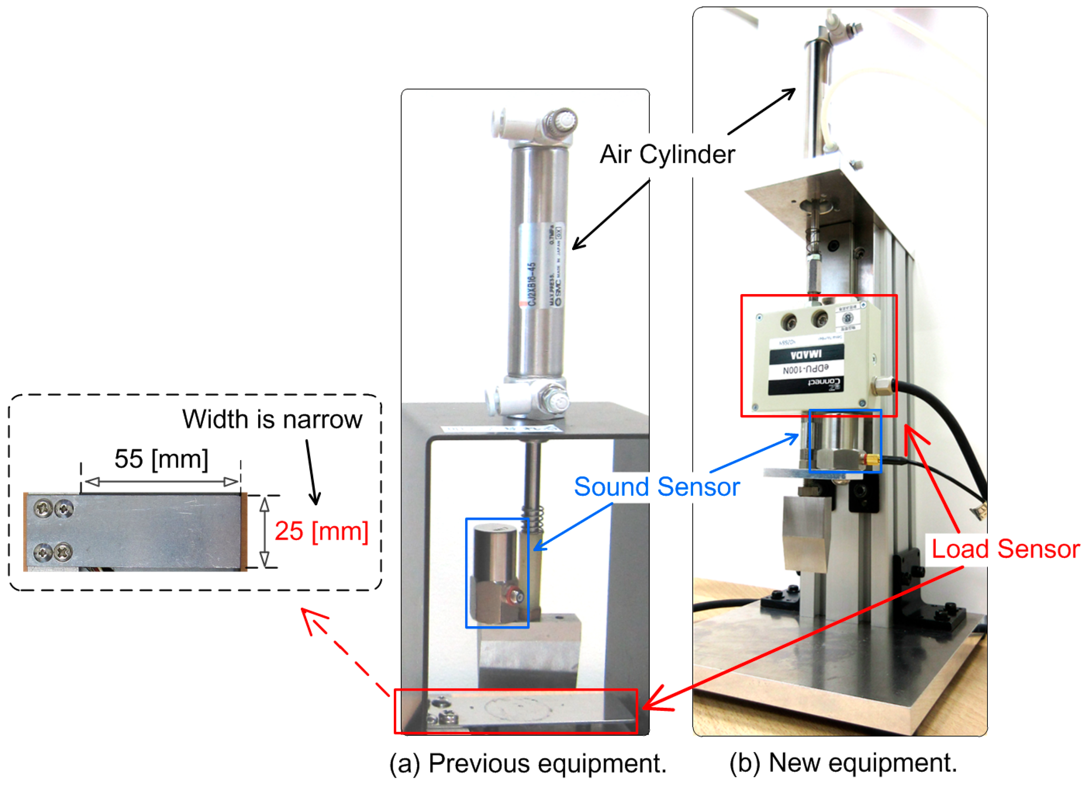
The load sensor used in our previous equipment [
8] was very narrow and fragile, as shown in
Figure 1a, and could accommodate only small food specimens. The current paper developed equipment built from the ground up [
10].
Figure 1b illustrates the system, in which the load sensor is attached to the top of the probe for examining differently sized food specimens. Rheometers are commonly used in food manufacturing companies for measuring the force response of the food [
11]; nevertheless, rheometers are not built with a sound sensor, unlike our equipment. Therefore, we could regard our equipment as a next-generation rheometer capable of observing load change and sound signals simultaneously. The equipment is very simple, durable, user-friendly, and inexpensive. The novelty of the current study is emphasized on the fusion of our original simple equipment and the artificial neural network model. In particular, the proposed model considers both the sound and load.
We first constructed a simple system using a neural network model that can quantify texture into numerical levels, e.g., “crispness = 0.8 or crunchiness = 0.5”. If such quantification is realized, food texture evaluation can be elevated to a merchandise level, and further development can be accomplished. We conducted an experiment to validate the efficiency of our proposed simple system.
As this study focuses on sound analysis, we investigated recent studies on sound signal processing using AI techniques, and then discovered several studies on audio feature analysis using a spectrogram. A spectrogram image obtained by short-time Fourier transform contains rich information regarding sound characteristics [
12,
13,
14]; for this, a convolution neural network (CNN) [
15] is employed to classify the sound from the inputted spectrogram. Justin and Juan [
16] addressed the classification of an environmental sound using CNN, into which a spectrogram-like image (mel-spectrogram) is inputted. CNN is useful for texture analysis of biometrics such as finger prints, palm texture [
17], and the iris [
18] to identify persons.
Shervin et al. [
19] suggested the application of CNN in distinguishing commercial scenes from main video contents, considering video slide images and spectrogram images. Likewise, Shawn et al. [
20] classify the musical performance scenes from video stream by CNN, which deals with performance scene images and spectrograms of audio. Such an interesting cross-modal method is possible in our study by combining the sound spectrogram and load change curve images. Afterward, these images will be processed by CNN for texture estimation. This study also addressed applying CNN for classifying snacks. The CNN analyzes an image that comprises the spectrogram of sound and visualized load intensity with color gradation. The capability of CNN for texture estimation is discussed.
2. System Structure
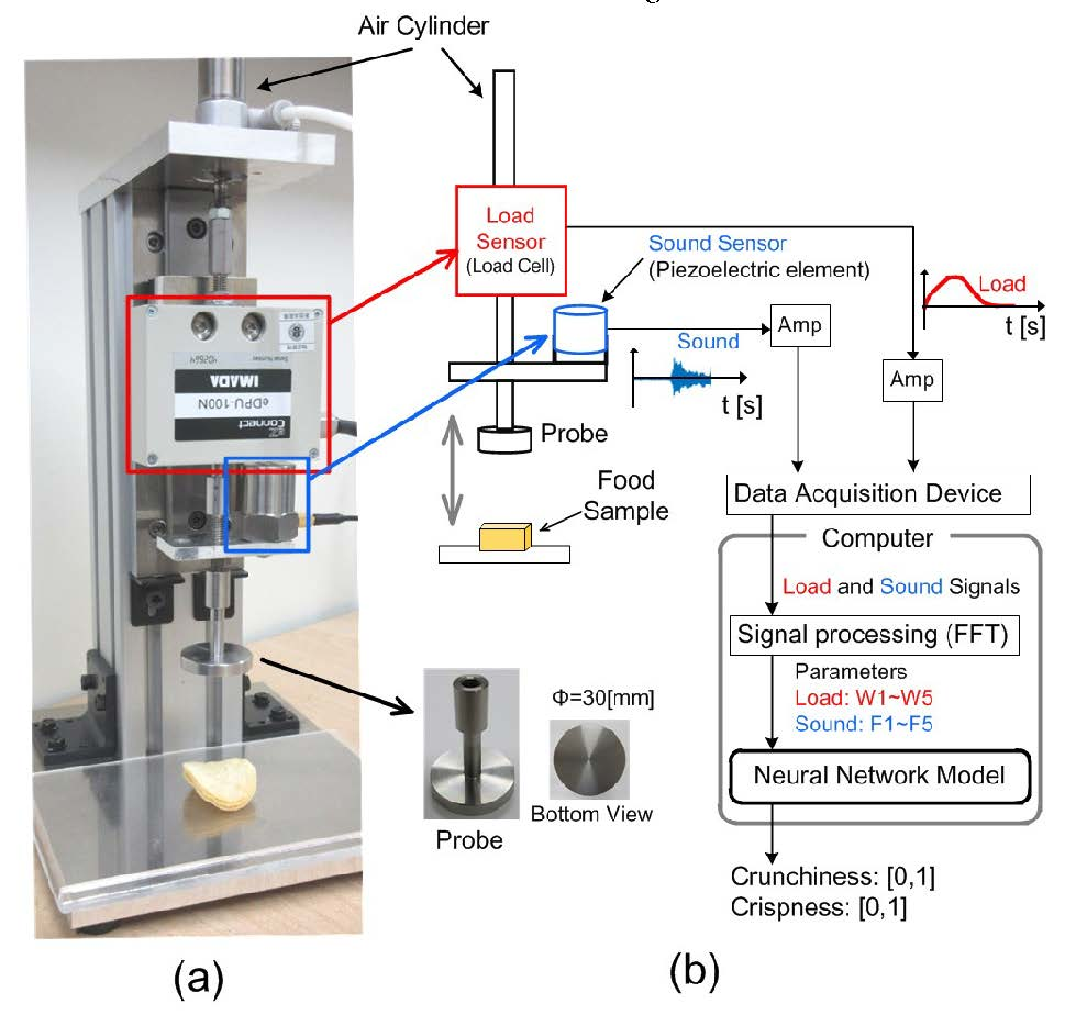
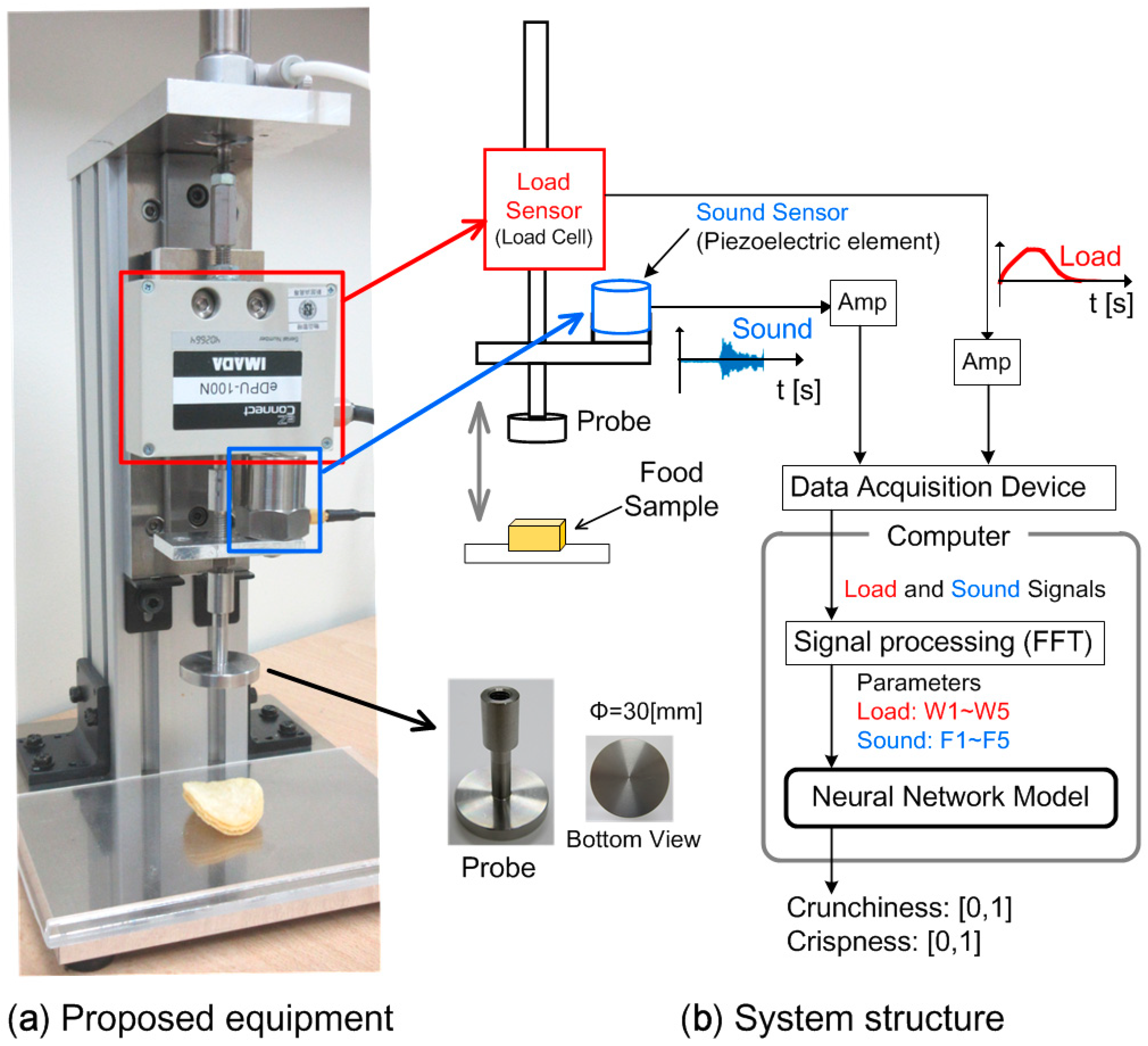
Figure 2 shows the system construction. In
Figure 2a, the equipment comprises an air cylinder that moves the metal probe up and down; under the flat and round metal probe is the food sample, i.e., potato chips. The air cylinder moves the probe up and down once it gains air pressure. On the other hand, the load sensor is a load cell fixed between the probe and the air cylinder rod, while the sound sensor is fixed on the metal probe. The system structure is shown in
Figure 2b. Signals from the sound and load sensors are amplified and transmitted to the computer via a data acquisition device. As noise is not filtered, the experiment should be performed in a quiet environment. The computer calculates input parameters of the neural network model: W1–W5 and F1–F5 express the characteristics of the load change and the sound features, respectively. The model then outputs the texture level range of (0,1) for “crunchiness” and “crispness”. Here, “crunchy” texture refers to a feeling with a certain load accompanied by a loud sound, while “crispy” texture is the feeling with small load accompanied by high-frequency sound.
Food viscosity or elasticity are measured by a rheometer [
11], which is generally used to measure only the force response of the food through an electrical motor that moves the probe. In our proposed equipment, we focus on measuring sound and relate it to “crunchiness” or “crispness” of the food specimen. For this reason, we employ the air cylinder instead of the electrical motor, which causes mechanical noise.
As shown in
Figure 3, if such an intelligent system is connected to the internet, then a user holding the equipment can obtain texture information from the server quickly due to the neural network model trained by a big amount of data.
3. Experiment
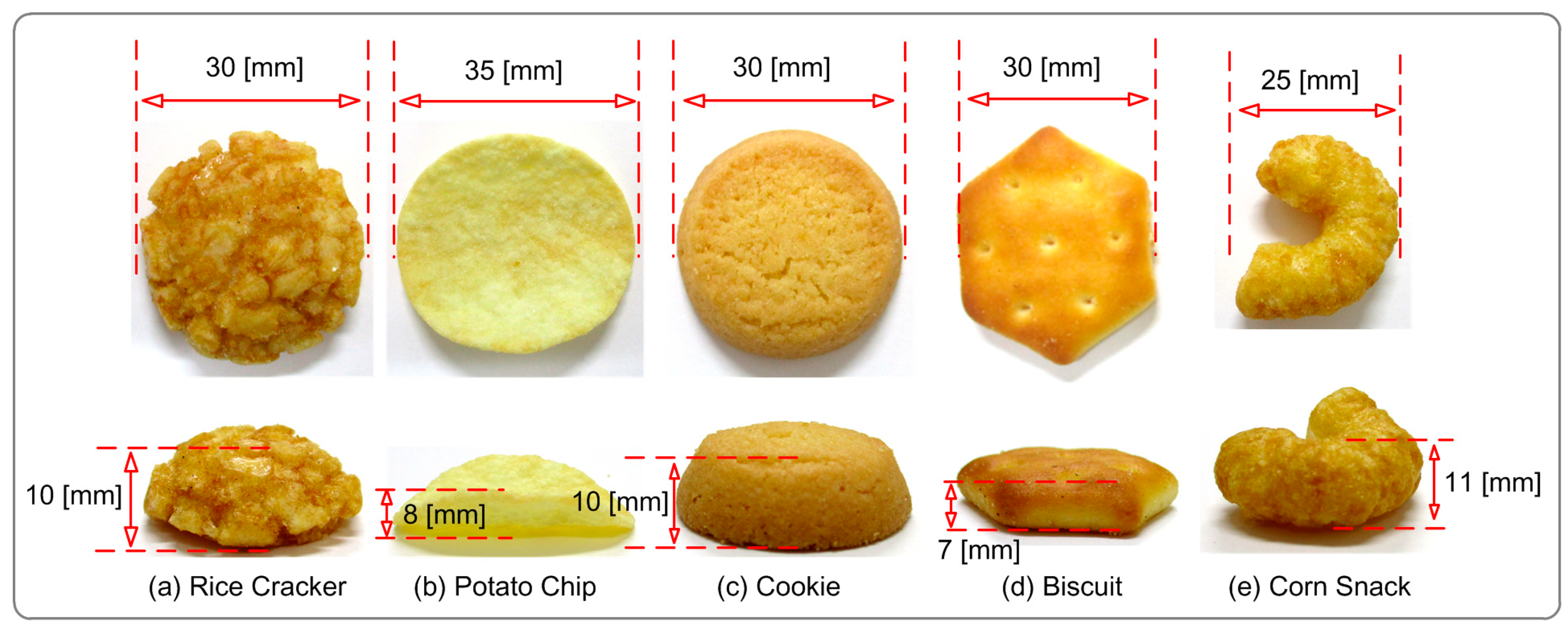
Rice crackers, potato chips, cookies, biscuits, and corn snacks purchased from a local supermarket were the food specimens evaluated by the system (
Figure 4).
Table 1 shows the number of samples and texture information of each food specimen after the experiment. Specifically, 200 rice crackers, 200 potato chips, 200 cookies, 200 biscuits, and 200 corn snacks were sampled.
Table 2 enumerates the conditions for the load and sound evaluation of the food samples.
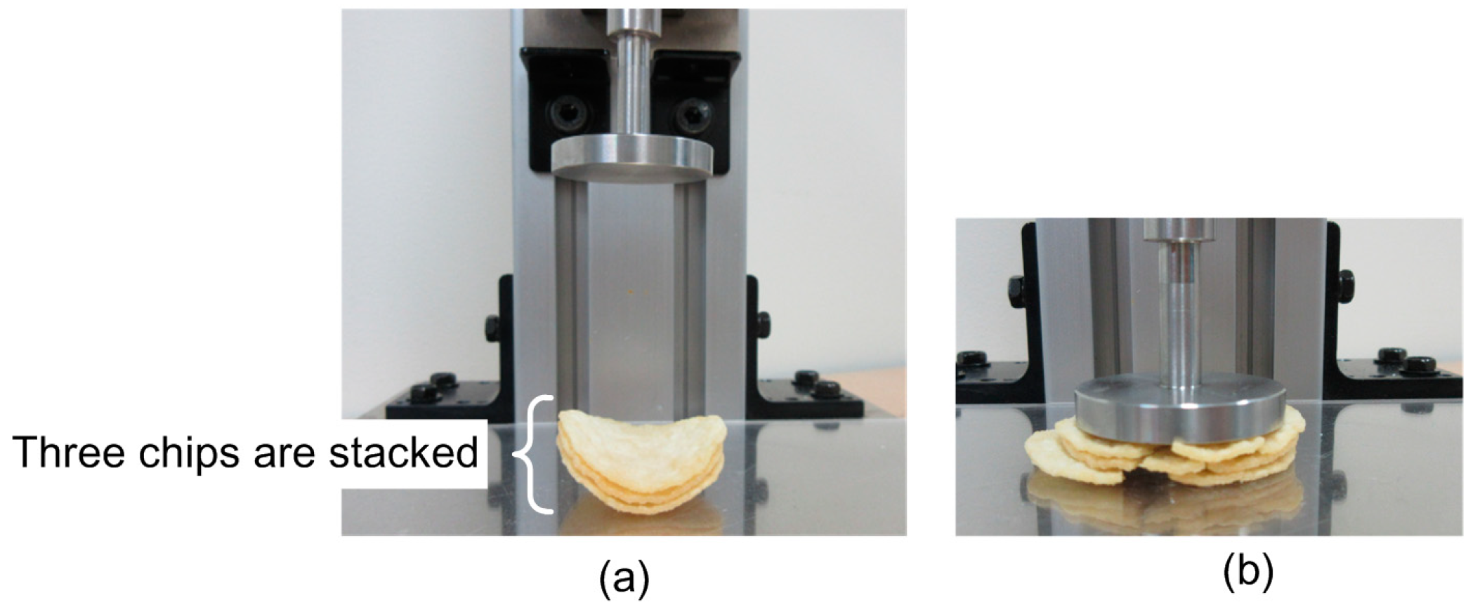
Figure 5a shows the image of three stacked potato chips being crushed by the equipment; this was carried out 200 times, leading to 200 data for the potato chips samples.
The experiment of each sample was conducted 200 times, for a total of 200 data. The samples are numbered accordingly, as illustrated in
Table 1.
Figure 6 displays graphs of five specimens of the experiment. The graph at the top illustrates the curve of the load (red line) and the sound (blue line), as shown in
Figure 6a, which indicates that as the probe touched the sample, the load increased and a loud sound occurred. The middle graph in
Figure 6a shows automatically extracted signals for 2.0 s; the extraction method is explained in the following paragraph. By focusing on the 2.0 s period while the snack is being pressed, we do not have to consider the noise influence except at the 2.0 s period. The bottom graph in
Figure 6a shows the FFT (Fast Fourier Transform) results of the extracted 2.0 s sound data. Likewise, the results for the potato chips, cookie, biscuit, and corn snack samples are displayed in
Figure 6b–e, respectively.
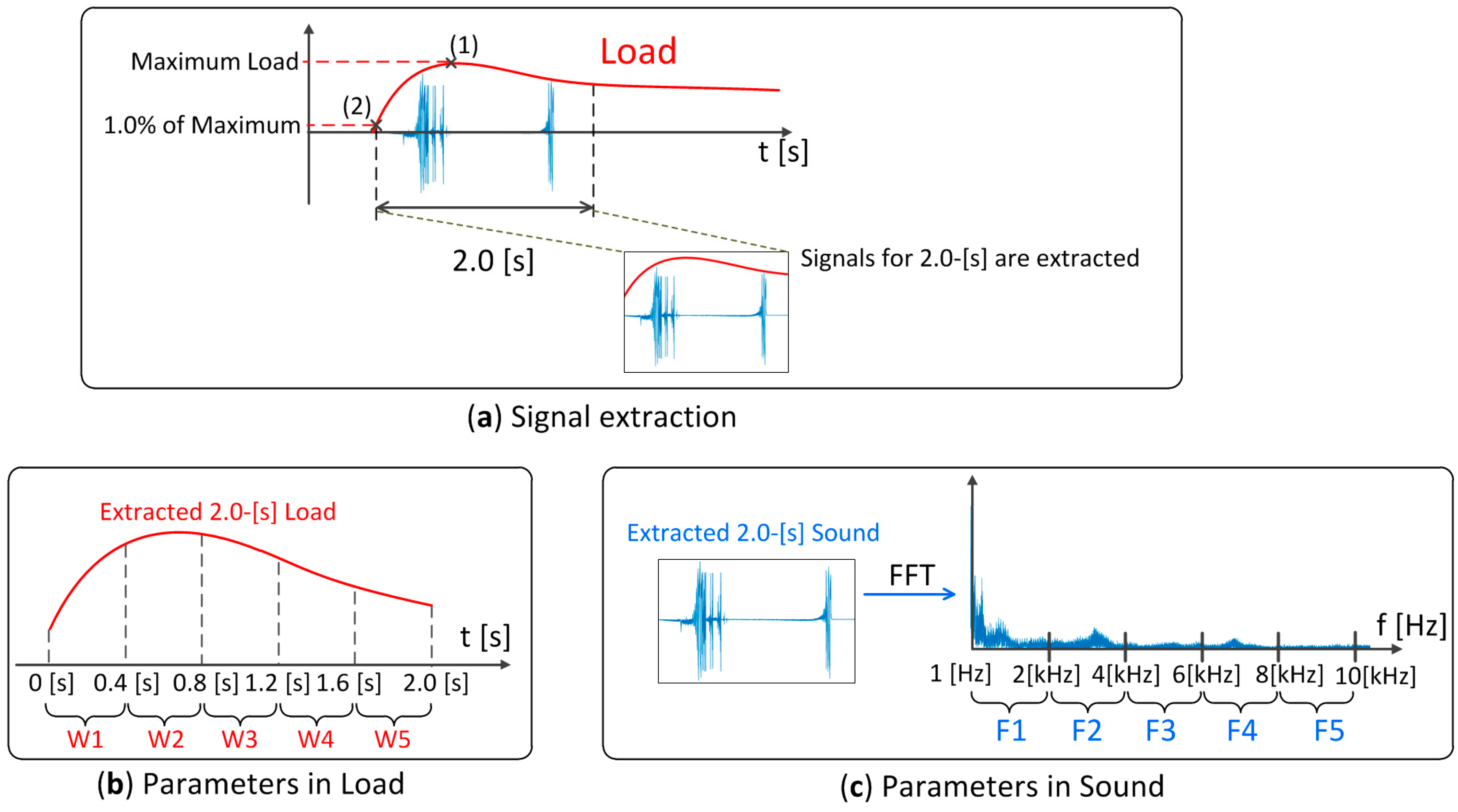
The signal data for 2.0 s were extracted from the entire 10 s data as shown in
Figure 7a.
- (i)
The maximum load point (1) was determined.
- (ii)
Point, at 1.0 % of maximum load, was identified.
- (iii)
Finally, signals for 2.0 s from point (2) were extracted.
The load curve of the extracted 2.0 s signals was divided into five sections, as shown in
Figure 7b. Subsequently, parameters W1–W5 in the load were calculated as follows:
- -
W1 is the average of the load between 0.0 s and 0.4 s.
- -
W2 is the average between 0.4 s and 0.8 s.
- -
W3 is the average between 0.8 s and 1.2 s.
- -
W4 is the average between 1.2 s and 1.6 s.
- -
W5 is the average between 1.6 s and 2.0 s.
The extracted 2.0 s sound signal data were converted by FFT, resulting in a frequency range of 1–10 kHz, which was also divided into five sections, as shown in
Figure 7c. F1–F5 in the sound were calculated as follows:
- -
F1 is the integration of FFT result between 1 Hz and 2 kHz.
- -
F2 is the integration of results between 2 kHz and 4 kHz.
- -
F3 is the integration of results between 4 kHz and 6 kHz.
- -
F4 is the integration of results between 6 kHz and 8 kHz.
- -
F5 is the integration of results between 8 kHz and 10 kHz.
Figure 8 shows the average values and standard deviations (STDs) of the parameters W1–W5 for (a) rice cracker, (b) potato chips, (c) cookie, (d) biscuit, and (e) corn snack, respectively. As observed, averages of W were different depending on each specimen.
Figure 9 shows the average values and STDs of F1–F5 for the (a) the rice cracker, (b) potato chips, (c) cookie, (d) biscuit, and (e) corn snack, respectively. Likewise, F1–F5 differed in the specimens.
The STDs showed that the parameters characterized different types of specimens, with respect to the form, size, and density. For texture estimation, we employed the neural network model. In a conventional texture analysis, multiple regression is employed as enormous sample data are analyzed [
21]; determining characteristics related to a target texture is a very complicated task. The neural network model simplifies this task and works well with the parameters W1–W5, and F1–F5 is obtained by a very simple calculation.
4. Neural Network Model
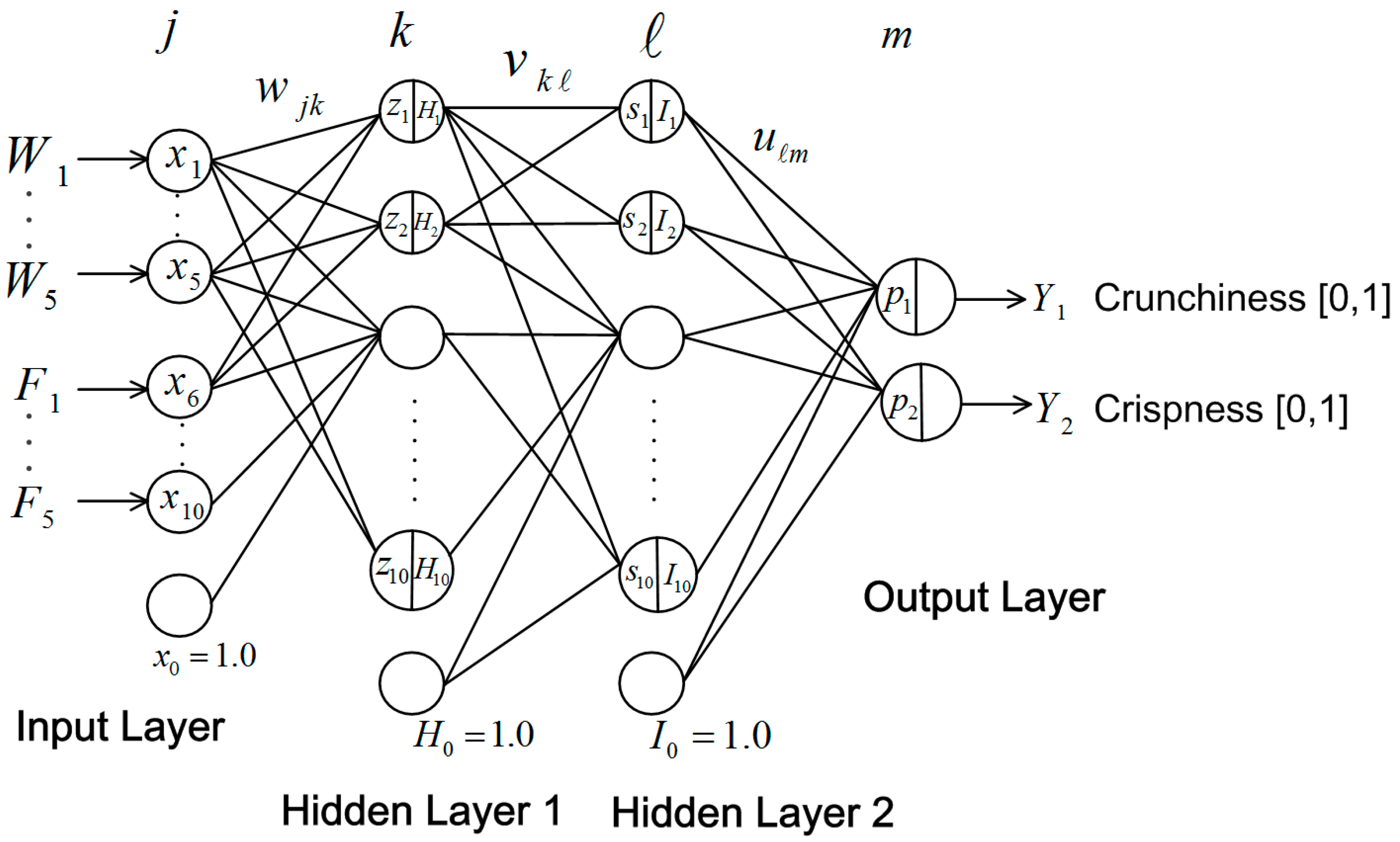
The neural network model for texture degree estimation is shown in
Figure 10. The input layer comprises 10 nodes for W1–W5 and F1–F5, and a bias node. Hidden layers 1 and 2 comprise 10 nodes and a bias node, respectively. The output layer comprises two nodes expressing the degree range (0,1) of “crunchiness” and “crispness”.
The transfer function of hidden layers 1, 2, and the output layer is expressed in Equations (1) – (3), respectively, where
is
j-th input node value,
is the output value of
k-th node of hidden layer 1,
is the output value of the
-th node of hidden layer 2, and
and
are the model outputs:
where
,
and
are the connection weights between the input layer and hidden layer 1, between hidden layers 1 and 2, and between hidden layer 2 and the output layer, respectively. The connection weights were adjusted to minimize the difference (i.e., error) between the expected value and the actual neural network output
via the back-propagation algorithm [
22].
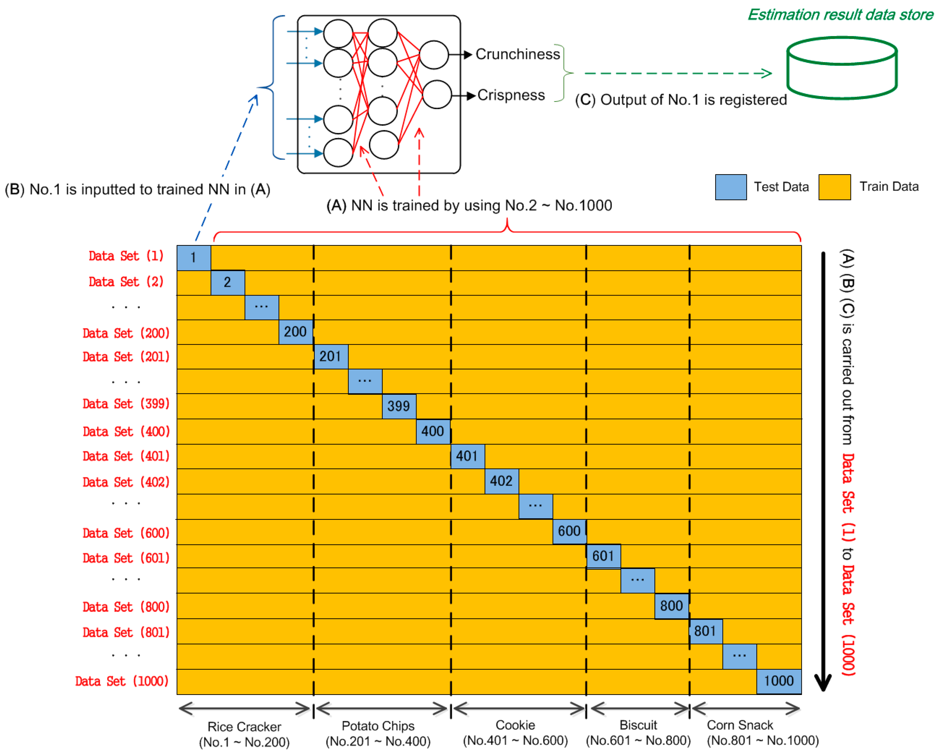
For a limited amount of data, such as in our case, the neural network model is verified via cross-validation [
23]. We implemented the leave-one-out cross-validation (
Figure 11) normally adopted for obtaining a reliable estimation [
24].
For Data Set (1), initially, (W1–W5, F1–F5) of sample Nos. 2–1000 were used for training the connection weights of the neural network in step (A). Subsequently, (W1–W5, F1–F5) of No. 1 were inputted to the trained network in step (B). Finally, crunchiness and crispness outputs of the network were registered in the estimation result data store in step (C). Similarly, (A)–(C) were repeated from Data Sets (2)–(1000). This Leave-One-Out Cross-Validation (LOOCV) was thus considered as 1000-fold cross-validation. The above procedure could be explained as follows:
Step 0:
Step 1: Select i-th sample data out of all 1000 samples
Step 2: Prepare the next 999 train input vectors except the
i-th data
Step 3: Prepare the next 999 correct output vectors
where,
is assigned for the rice crackers,
is assigned for the potato chips,
is assigned for the cookies,
is assigned for the biscuits, and
is assigned for the corn snacks. These values were in accordance with
Table 1.
Step 4: Initiate the connection weights w, v, and u, which are random values. Train the neural network model by the back-propagation algorithm by adjusting w, v, and u so that is outputted when the corresponding is inputted. In particular, the iteration to train the network is 100 epochs. It is necessary to observe the decreasing error as the epoch proceeds.
Step 5: Input W1–W5 and F1–F5 of the i-th sample data into the neural network model trained in previous step i.e., Step 4. (*Note that the i-th sample data is not used to train the neural network in Step 4.) The output texture value set (i.e., estimated texture result of the i-th sample) is registered in the estimation result data store.
When
, the routine is completed, otherwise
and return to
Step 1.
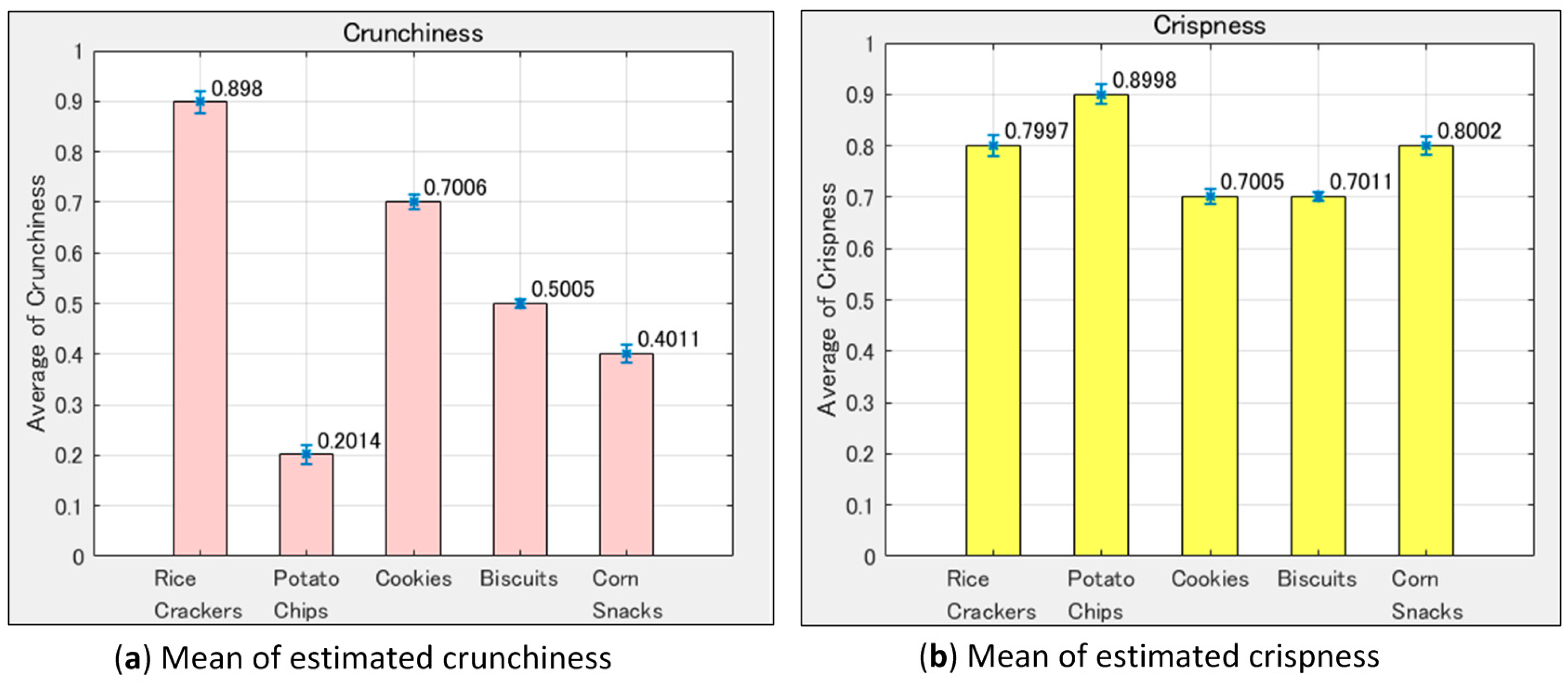
Table 3 shows the averages of texture values in the estimation result data store. Although the sample data not used for training were inputted to the neural network model, the model outputs generally expected values.
Based on the result of this implementation, the neural network model estimated the expected textures almost correctly, even though there was a dispersion in parameters W1–W5 and F1–F5.
Figure 12 displays the averages and STDs in
Table 3.
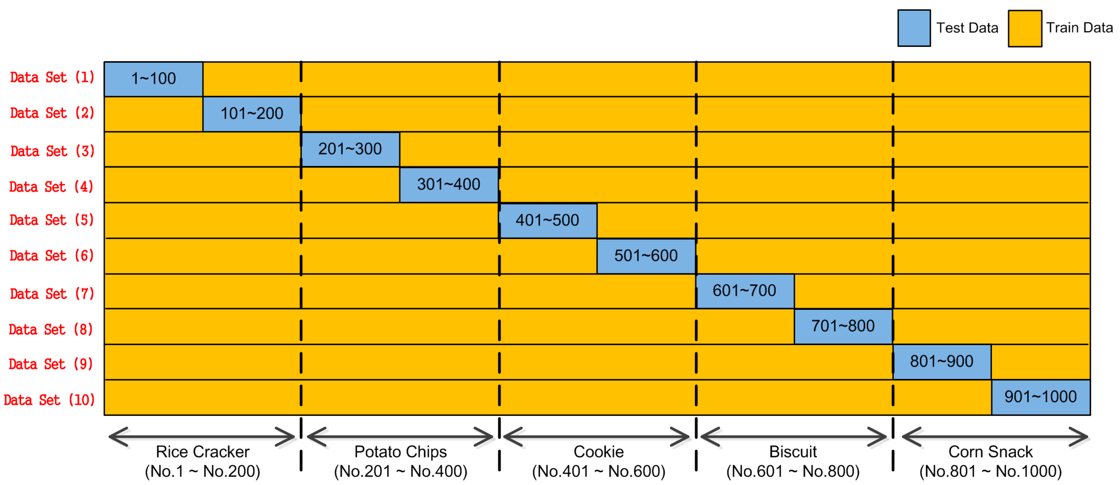
To validate the general flexibility of the neural network model, we performed another 10-fold cross-validation for Data Sets (1)–(10), as shown in
Figure 13. For Data Set (1), Nos. 101–1000 were used to train the neural network, while Nos. 1–100 were used as test data and thus, inputted to the trained neural network afterward. The outputted results were registered in the estimation result data store. Similarly, for Data Set (2), Nos. 101–200 were used to test the neural network, previously trained by Nos. 1–100 and Nos. 201–1000. This process was iterated from Data Sets (1)–(10) in the same way explained above from Step 0 to Step 5. For each data set, the test data output were preserved in the estimation result data store. The estimation result data store for the validation is illustrated in
Figure 14.
Since the training data were decreased compared with the Leave-One-Out Cross-Validation (LOOCV) in
Figure 11 (i.e., LOOCV), the estimated result dispersed as STDs are shown in
Figure 14. However, estimation values generally gathered around the expected values, even though W1–W5 and F1–F5 showed dispersion even for the same food specimen, as previously shown in
Figure 8 and
Figure 9. In summary, the combination of our equipment and NN (Neural Network) worked well to quantify the texture levels.
5. CNN
The spectrogram has rich sound features [
12,
13,
14]. To enhance the system capabilities, we considered introducing CNN [
15], which deals with images. As a first step, we tried to classify snacks using CNN.
Since we have only 1000 data points, we adopted AlexNet [
25], which is a pre-trained CNN. We employed the Neural Network Toolbox in MATLAB developed by MathWorks. We conducted Transfer Learning using AlexNet [
26].
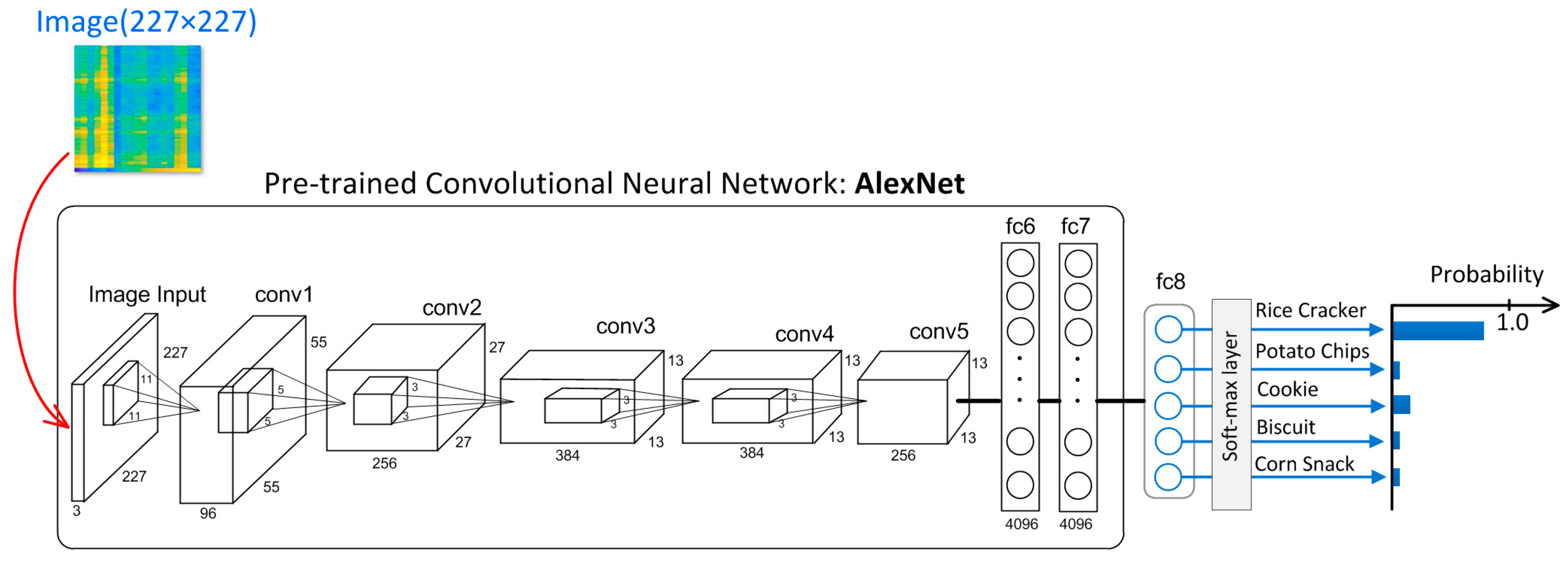
Figure 15 shows the CNN classifying the snacks. Note that the ReLU operation, cross-channel normalization, and max-pooling layers are omitted in
Figure 15. CNN comprises the input layer for the 227 × 227 RGB image and soft-max output layer. The soft-max layer outputs classified values of rice cracker, potato chips, cookies, biscuit, and corn snacks within a range of (0,1). The item with the highest classified value is judged as an inputted snack. For instance, the value of the rice cracker is highest in
Figure 15; thereby, the inputted image is classified as a rice cracker.
The convolution layers (conv1–conv5) and fully connected layers (fc6 and 7) are original parts which are pre-trained with a massive number of image data. We only attached fc8 and the soft-max layer with original AlexNet.
The input image (227 × 227 RGB) comprises the spectrogram and visualized load intensity (
Figure 16b), which are obtained from extracted 2.0 s signals (
Figure 16a). FFT is performed in each section from (1)–(19), as shown in
Figure 16a, where the period of each section is 0.2 s, and then there are 0.1 s overlaps between the adjacent sections. FFT results of (1)–(19) are visualized, as shown in
Figure 16b. In addition, this image also includes information in the load intensity, which is visualized in the bottom part of the image.
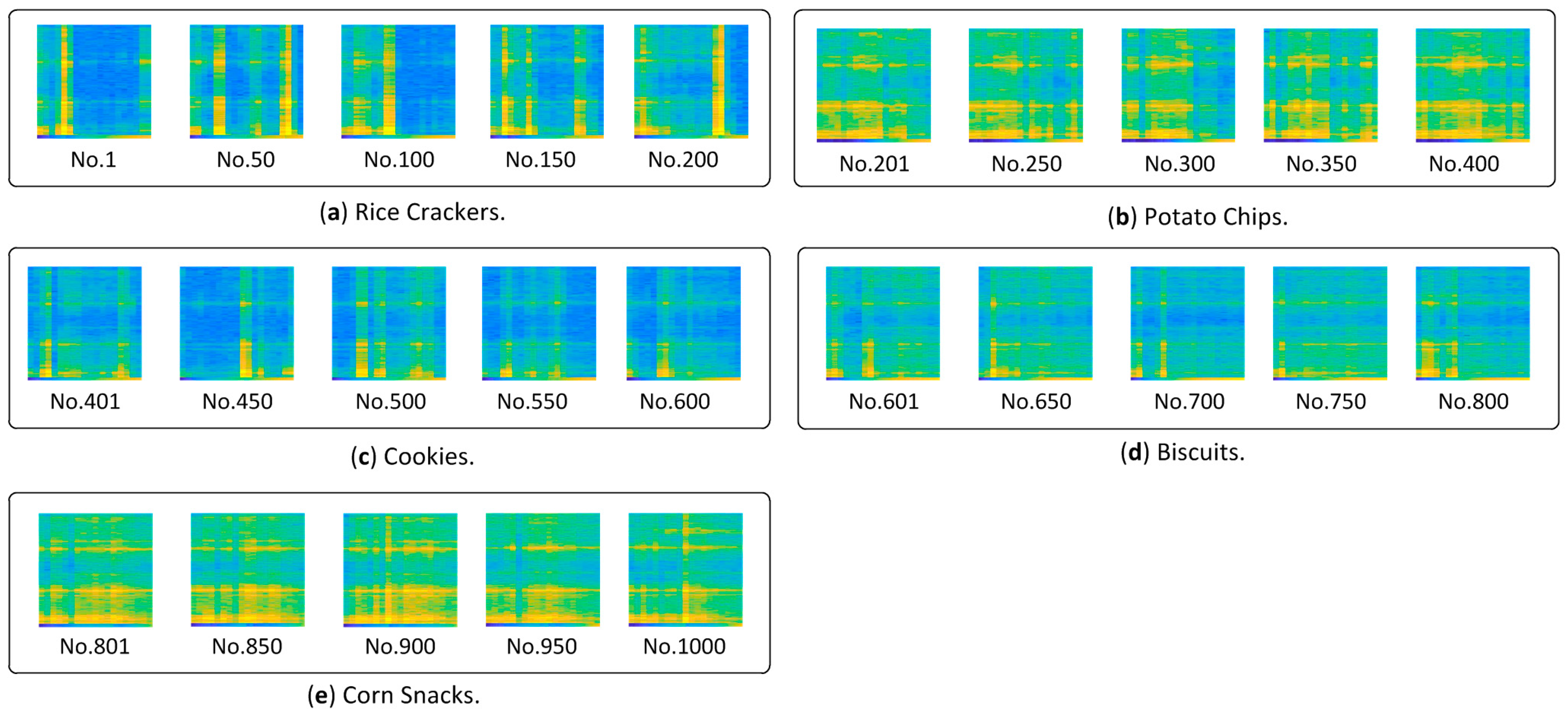
The images of snacks are generated automatically and numbered as shown in
Table 4, and then some of the generated images are shown in
Figure 17.
Table 5 enumerates the conditions for validation of CNN. The 10-fold cross-validation in
Figure 13 is performed. The result is shown in
Table 6. CNN performed very well. The mean of the accuracies in Data Sets (1)–(10) is 98.30%. The CNN is useful to modify or revise the outputted texture values from NN model described in previous
Section 4. It is found that incorporating CNN must improve our system.
6. Conclusions
This paper proposed a food-texture-estimation system which is comprised of improved equipment and a simple neural network model. The system can process load changes and sound signals simultaneously for estimating textures, i.e., crunchiness and crispness. The classical neural network model was applied in the experiments to estimate the expected texture values of food specimens, i.e., rice crackers, potato chips, cookies, biscuits, and corn snacks. The model works well. Moreover, CNN is applied to classify the spectrogram image, including rich sound features, to expand our model capabilities. The CNN model performed very well. In the future, we will address the texture evaluation using CNN. Conventionally, food texture evaluation is manually performed by humans and is cumbersome. The neural network model simplifies this task. In this work, a moderate estimation was performed.


