A Fusion Load Disaggregation Method Based on Clustering Algorithm and Support Vector Regression Optimization for Low Sampling Data

Abstract
1. Introduction
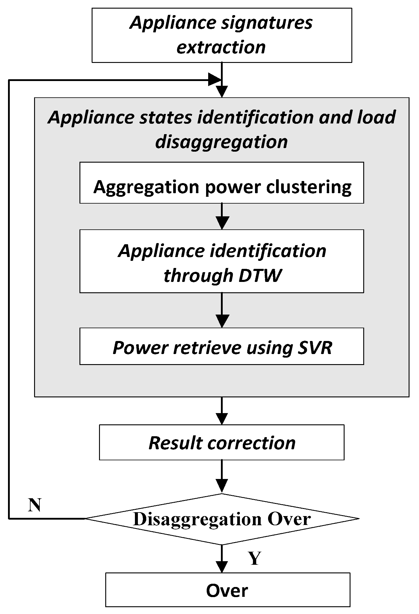
2. Proposed Method
2.1. Power Consumption Pattern Signatures Extraction
2.2. Appliance States Identification and Load Disaggregation
2.2.1. Aggregation Power Clustering and Appliance Identification through DTW
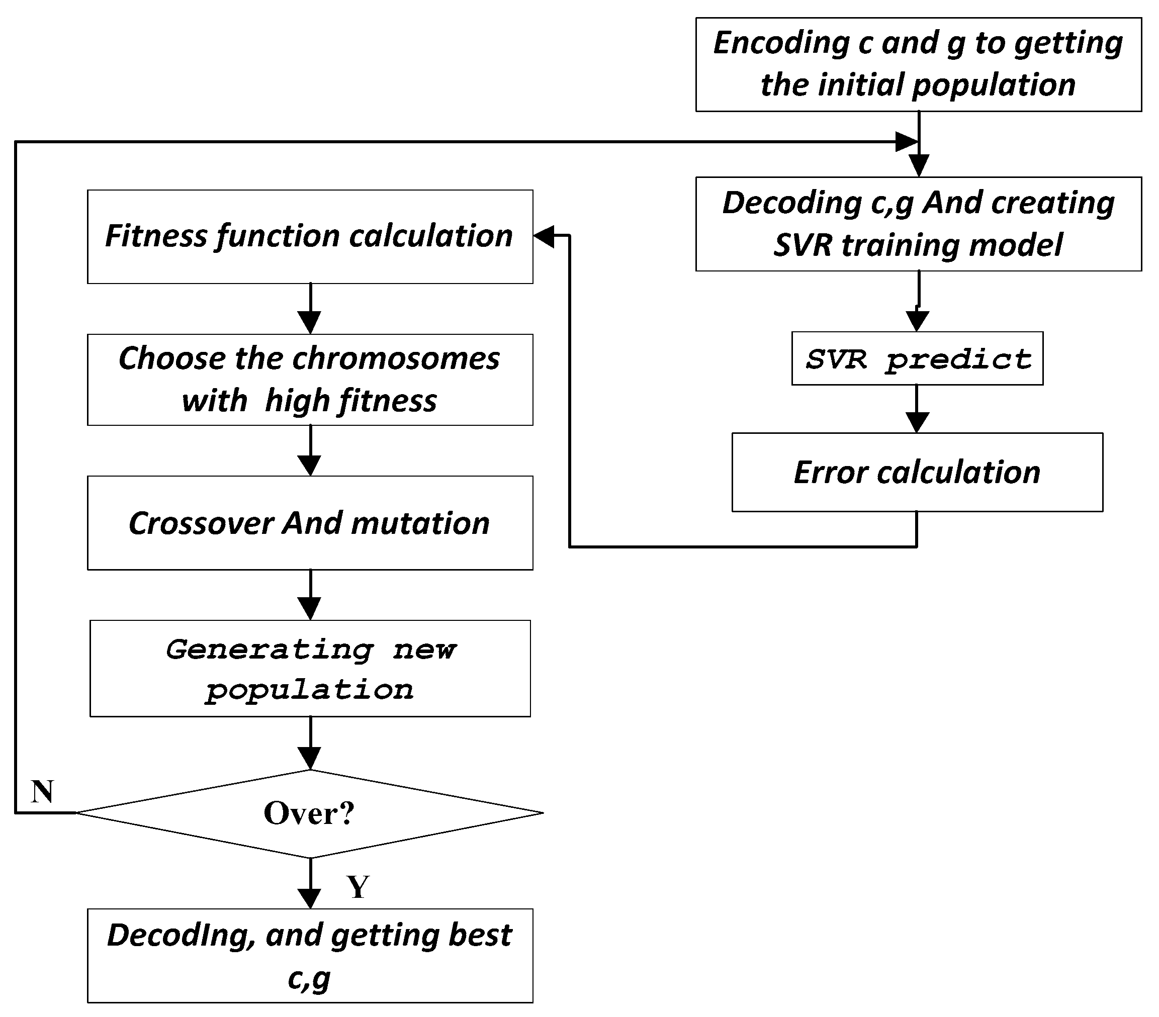
2.2.2. Power Retrieve
2.3. Result Correction
- Check the current total power time sequence, and negative values are considered estimation errors. In order to correct the estimation errors, the negative value was set as the average of the two numbers before and after it, and the estimation value was adjusted accordingly.
- If the subsequence obtained after clustering was truncated by a few values which had been estimated formerly, these values were considered estimation errors.
- The values, identified as multiple simultaneously operating states of the same appliance, were considered estimation errors.
3. Experiment Setting
3.1. Data
3.2. Performance Evaluation Metrics
4. Results and Discussion
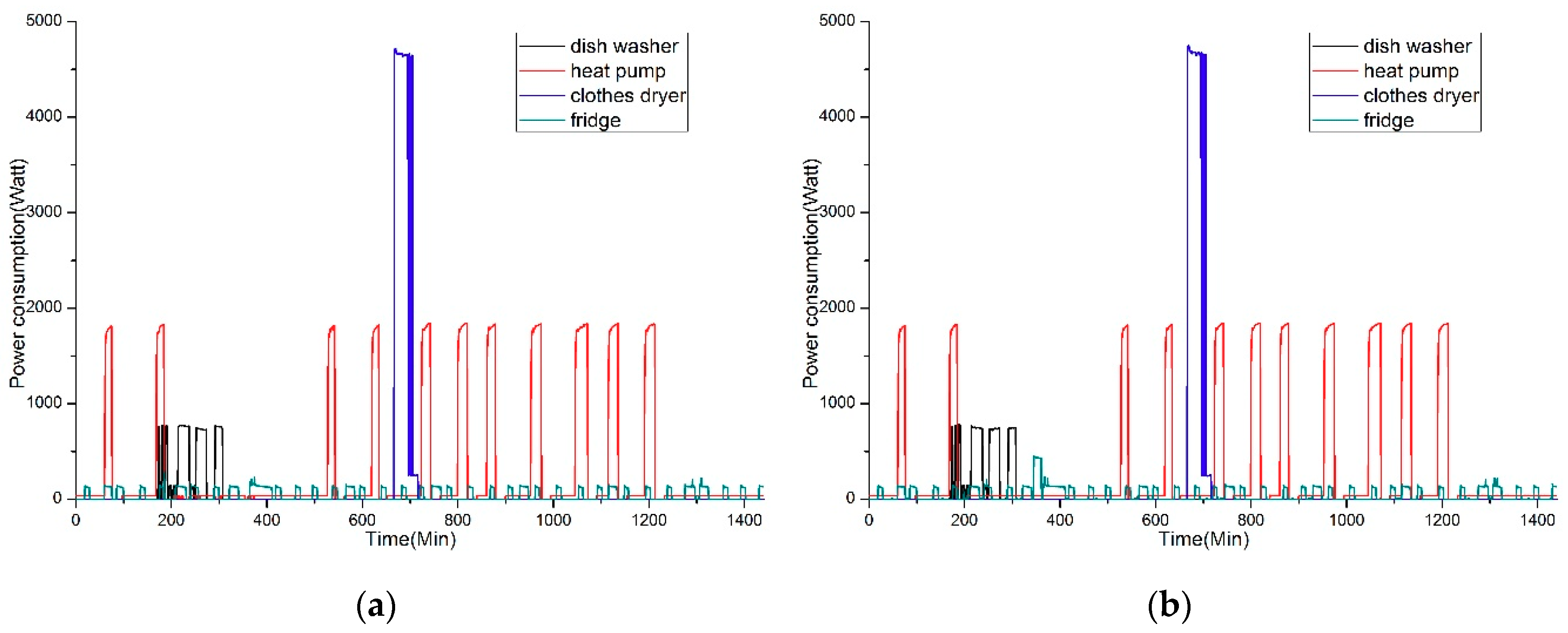
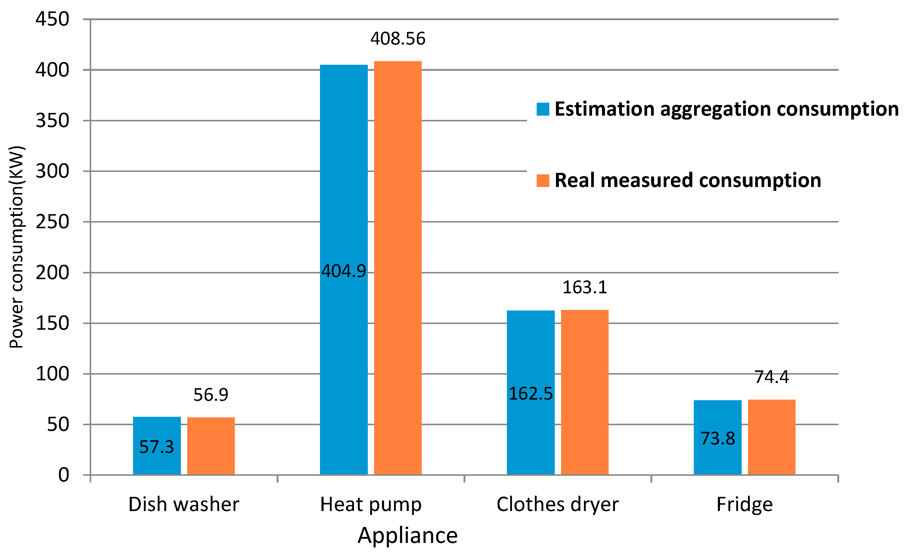
4.1. The Load Disaggregation Results
4.2. Performance Comparison
4.3. Time Consumption Comparison of Power Trajectory Estimation
4.4. Estimation Performance Comparison between OSVR and SVR
4.5. Method Limitations and Ways to Address Them
5. Conclusions
Author Contributions
Funding
Conflicts of Interest
References
- Armel, K.C.; Gupta, A.; Shrimali, G.; Albert, A. Is disaggregation the holy grail of energy efficiency? The case of electricity. Energy Policy 2013, 52, 213–234. [Google Scholar] [CrossRef]
- Chakravarty, P.; Gupta, A. Impact of Energy Disaggregation on Consumer Behavior. Available online: https://www.mendeley.com/catalogue/impact-energy-disaggregation-consumer-behavior/ (accessed on 15 February 2019).
- Hart, G.W. Nonintrusive appliance load monitoring. Proc. IEEE 1992, 80, 1870–1891. [Google Scholar] [CrossRef]
- Egarter, D.; Bhuvana, V.P.; Elmenreich, W. PALDi: Online load an unsupervised training method for adisaggregation via particle filtering. IEEE Trans. Instrum. Meas. 2015, 64, 467–477. [Google Scholar] [CrossRef]
- Egarter, D.; Elmenreich, W. Autonomous load disaggregation approach based on active power measurements. Presented at the 2015 IEEE International Conference on Pervasive Computing and Communication Workshops Workshop (PerCom Workshops), St. Louis, MO, USA, 23–27 March 2015; pp. 293–298. [Google Scholar]
- Elafoudi, G.; Stankovic, L.; Stankovic, V. Power disaggregation of domestic smart meter readings using dynamic time warping. Presented at the Communications, Control and Signal Processing (ISCCSP), Athens, Greece, 21–23 May 2014; pp. 36–39. [Google Scholar]
- Figueiredo, M.; Ribeiro, B.; de Almeida, A. Electrical signal source separation via nonnegative tensor factorization using on site measure-ments in a smart home. IEEE Trans. Instrum. Meas. 2014, 63, 364–373. [Google Scholar] [CrossRef]
- Guo, Z.; Wang, Z.J.; Kashani, A. Home appliance load modelingfrom aggregated smart meter data. IEEE Trans. Power Syst. 2015, 30, 254–262. [Google Scholar] [CrossRef]
- Wang, A.L.; Chen, B.X.; Wang, C.G.; Hua, D.D. Non-intrusive load monitoring algorithm based on features of V-I trajectory. Electr. Power Syst. Res. 2018, 157, 134–144. [Google Scholar] [CrossRef]
- Wang, H.; Yang, W.; Yang, Q. An Optimal Load Disaggregation Method Based onPower Consumption Pattern for Low Sampling Data. Sustainability 2019, 11, 251. [Google Scholar] [CrossRef]
- Tabatabaei, S.M.; Dick, S.; Xu, W. Towards Non-Intrusive Load Monitoring via Multi-Label Classification. IEEE Trans. Smart Grid 2017, 1, 26–40. [Google Scholar] [CrossRef]
- Maitre, J.; Glon, G.; Gaboury, S.; Bouchard, B.; Bouzouane, A. Efficient appliances recognition in smart homes based on active andreactive power, fast fourier transform and decision trees. Presented at the AAAI Workshops: Artificial Intelligence Applied to Assistive Technologies and Smart Environments, Austin, TX, USA, 25–30 January 2015; pp. 24–29. [Google Scholar]
- Meehan, P.; Ardle, C.M.; Daniels, S. An efficient, scalable time-frequency method for tracking energy usage of domestic appliancesusing a two-step classification algorithm. Energies 2014, 7, 7041–7066. [Google Scholar] [CrossRef]
- Semwal, S.; Singh, M.; Prasad, R.S. Group control and identifi-cation of residential appliances using a nonintrusive method. Turk. J. Electr. Eng. Comput. Sci. 2015, 23, 1805–1816. [Google Scholar] [CrossRef]
- Wild, B.; Barsim, K.S.; Yang, B. A new unsupervised event detector for non-intrusive load monitoring. Presented at the 2015 IEEE Global Conference on Signal and Information Processing (GlobalSIP), Orlando, FL, USA, 14–16 December 2015; pp. 73–77. [Google Scholar]
- Gillis, J.M.; Alshareef, S.M.; Morsi, W.G. Nonintrusive Load Monitoring Using Wavelet Design and Machine Learning. IEEE Trans. Smart Grid 2017, 7, 320–328. [Google Scholar] [CrossRef]
- Gillis, J.M.; Morsi, W.G. Non-Intrusive Load Monitoring Using Semi-Supervised Machine Learning and Wavelet Design. IEEE Trans. Smart Grid 2017, 8, 2648–2655. [Google Scholar] [CrossRef]
- Rahayu, D.; Narayanaswamy, B.; Krishnaswamy, S.; Labbé, C.; Seetharam, D.P. Learning to be energy-wise: Discriminative methods for load disaggregation. Presented at the 3rd International Conference on Future Energy Systems: Where Energy, Computing and Communication Meet, Madrid, Spain, 9–11 May 2012; pp. 1–4. [Google Scholar]
- Berges, M.; Goldman, M.; Matthews, H.; Soibelman, L.; Anderson, K. User-centered nonintrusive electricity load monitoring for resi-dential buildings. J. Comput. Civ. Eng. 2011, 25, 471–480. [Google Scholar] [CrossRef]
- Chang, H.-H.; Lee, M.-C.; Chen, N.; Chien, C.-L.; Lee, W.-J. Feature extraction based Hellinger distance algorithm for non-intrusive agingload identification in residential buildings. Presented at the IEEE Industry Applications Society Annual Meeting, Addison, TX, USA, 18–22 October 2015; pp. 1–8. [Google Scholar]
- Nguyen, M.; Alshareef, S.; Gilani, A.; Morsi, W.G. A novel feature extraction and classification algorithm based on power components using single-point monitoring for NILM. Presented at the IEEE 28th Canadian Conference on Electrical and Computer Engineering (CCECE), Halifax, NS, Canada, 3–6 May 2015; pp. 37–40. [Google Scholar]
- Jimenez, Y.; Duarte, C.; Petit, J.; Carrillo, G. Feature extraction for nonintrusive load monitoring based on S-transform. Presented at the Power Systems Conference (PSC), Clemson University, Clemson, SC, USA, 11–14 March 2014; pp. 1–5. [Google Scholar]
- Singh, M.; Kumar, S.; Semwal, S.; Prasad, R.S. Residential load signature analysis for their segregation using wavelet—SVM. In Power Electronics and Renewable Energy Systems; Kamalakannan, C., Suresh, L.P., Dash, S.S., Panigrahi, B.K., Eds.; Springer: New Delhi, India, 2015; pp. 863–871. [Google Scholar]
- Zoha, A.; Gluhak, A.; Nati, M.; Imran, M.A.; Rajasegarar, S. Acoustic and device feature fusion for load recognition. Presented at the IEEE 2012 6th IEEE International Conference Intelligent Systems, Sofia, Bulgaria, 6–8 September 2012; pp. 386–391. [Google Scholar]
- Yang, C.C.; Soh, C.S.; Yap, V.V. A non-intrusive appliance load monitoring for efficient energy consumption based on Naive Bayes classifier. Sustain. Comput. Inform. Syst. 2017, 14, 34–42. [Google Scholar] [CrossRef]
- Mauch, L.; Yang, B. A new approach for supervised power disaggregation by using a deep recurrent LSTM network. In Proceedings of the 2015 IEEE Global Conference on Signal and Information Processing (GlobalSIP), Orlando, FL, USA, 14–16 December 2015. [Google Scholar]
- Do Nascimento, P.P. Applications of Deep Learning Techniques on NILM. Ph.D.Thesis, Universidade Federal do Rio de Janeiro, Rio de Janeiro, Brazil, 2016. [Google Scholar]
- Xing, Z.; Pei, J.; Keogh, E. A brief survey on sequence classification. Acm Sigkdd Explor. Newsl. 2010, 12, 40–48. [Google Scholar] [CrossRef]
- Liu, B.; Luan, W.; Yu, Y. Dynamic time warping based non-intrusive load transient identification. Appl. Energy 2017, 195, 634–645. [Google Scholar] [CrossRef]
- Chang, H.H.; Yang, H.T. Applying a non-intrusive energy-management system to economic dispatch for a cogeneration system and power utility. Appl. Energy 2009, 86, 2335–2343. [Google Scholar] [CrossRef]
- Parson, O.; Ghosh, S.; Weal, M.; Rogers, A. An unsupervised training method for non-intrusive appliance load monitoring. Artif. Intell. 2014, 217, 1–9. [Google Scholar] [CrossRef]
- Cominola, A.; Giuliani, M.; Piga, D.; Castelletti, A.; Rizzoli, A.E. A Hybrid Signature-based Iterative Disaggregation algorithm for Non-Intrusive Load Monitoring. Appl. Energy 2017, 185, 331–344. [Google Scholar] [CrossRef]
- Li, J.; West, S.; Platt, G. Power decomposition based on SVM regression. In Proceedings of the IEEE International Conference on Modelling, Identification Control, Wuhan, China, 24–26 June 2012; pp. 1195–1199. [Google Scholar]
- Har-Peled, S.; Mazumdar, S. On coresets for k-means and k-median clustering. ProceedingS of the Thirty-Sixth ACM Symposium on Theory of Computing, Chicago, IL, USA, 13–16 June 2004; pp. 291–300. [Google Scholar]
- Wang, H.; Yang, W. An Iterative Load Disaggregation Approach Based on Appliance Consumption Pattern. Appl. Sci. 2018, 8, 542. [Google Scholar] [CrossRef]
- Boser, B.E. A training algorithm for optimal margin classifiers. In Proceedings of the ACM Fifth Workshop on Computational Lerning Theory, Pittsburgh, PA, USA, 27–29 July 1992; pp. 144–152. [Google Scholar]
- Vapnik, V.; Golowich, S.E.; Smola, A. Support Vector Method for Function Approximation, Regression Estimation, and Signal Processing. Adv. Neural Inf. Process. Syst. 1996, 9, 281–287. [Google Scholar]
- Goldberg, D.E. Genetic Algorithms in Search, Optimization, and Machine Learning; Addison-Wesley: Reading, MA, USA, 1989. [Google Scholar]
- Makonin, S.; Ellert, B.; Bajić, I.V.; Popowich, F. Electricity, water, and natural gas consumption of a residential house in Canada from 2012 to 2014. Sci. Data 2016, 3, 160037. [Google Scholar] [CrossRef] [PubMed]


| Appliance | Status | Average Power/W |
|---|---|---|
| Clothes dryer | Off | 0 |
| On-state 1 | 245 | |
| On-state 2 | 4586 | |
| Heat pump | Off | 0 |
| On-state 1 | 37 | |
| On-state 2 | 1767 | |
| Dish washer | Off | 0 |
| On-state 1 | 139 | |
| On-state 2 | 757 | |
| Fridge | Off | 0 |
| On-state1 | 130 |
| Metrics | F-score | PCE (%) | R2 |
|---|---|---|---|
| Dish washer | 0.995 | 0.057 | 0.996 |
| Heat pump | 0.980 | 0.521 | 0.975 |
| Clothes dryer | 1 | 0.083 | 0.999 |
| Fridge | 0.999 | 0.090 | 0.950 |
| Appliance | Period 1 | Period 2 | Period 3 |
|---|---|---|---|
| Dish washer | 0.996 | 0.991 | 0.991 |
| Heat pump | 0.984 | 0.976 | 0.973 |
| Clothes dryer | 1 | 1 | 1 |
| Fridge | 1 | 0.986 | 0.978 |
| Appliance | Period 1 | Period 2 | Period 3 |
|---|---|---|---|
| Dish washer | 0.052 | 0.055 | 0.074 |
| Heat pump | 0.511 | 0.505 | 0.544 |
| Clothes dryer | 0.070 | 0.203 | 0.211 |
| Fridge | 0.075 | 0.137 | 0.216 |
| Appliance | FHMM in Literature [32] | Proposed Method |
|---|---|---|
| Dish washer | 0.87 | 0.995 |
| Heat pump | 0.96 | 0.980 |
| Clothes dryer | 0.72 | 1 |
| Fridge | 0.98 | 0.999 |
| Appliance | Average Power Method in Literature [9] | DTW-Based Method in Literature [32] | Proposed Method |
|---|---|---|---|
| Dish washer | 0.074 | 0.242 | 0.057 |
| Heat pump | 0.453 | 0.1 | 0.521 |
| Clothes dryer | 0.463 | 0.2 | 0.083 |
| Fridge | 0.952 | 0.077 | 0.090 |
| Appliance | DTW-Based Method in Literature [32] | Proposed Method |
|---|---|---|
| Dish washer | 0.924 | 0.996 |
| Heat pump | 0.959 | 0.975 |
| Clothes dryer | 0.999 | 0.999 |
| Fridge | 0.938 | 0.950 |
| Power Estimation Method | SDTW | OSVR Based Method |
|---|---|---|
| Time(s) | 13.14296 | 2.91480 |
| Algorithm | OSVR | SVR |
|---|---|---|
| RMSE | 1.93 | 4.16 |
© 2019 by the authors. Licensee MDPI, Basel, Switzerland. This article is an open access article distributed under the terms and conditions of the Creative Commons Attribution (CC BY) license (http://creativecommons.org/licenses/by/4.0/).
Share and Cite
Yuan, Q.; Wang, H.; Wu, B.; Song, Y.; Wang, H. A Fusion Load Disaggregation Method Based on Clustering Algorithm and Support Vector Regression Optimization for Low Sampling Data. Future Internet 2019, 11, 51. https://doi.org/10.3390/fi11020051
Yuan Q, Wang H, Wu B, Song Y, Wang H. A Fusion Load Disaggregation Method Based on Clustering Algorithm and Support Vector Regression Optimization for Low Sampling Data. Future Internet. 2019; 11(2):51. https://doi.org/10.3390/fi11020051
Chicago/Turabian StyleYuan, Quanbo, Huijuan Wang, Botao Wu, Yaodong Song, and Hejia Wang. 2019. "A Fusion Load Disaggregation Method Based on Clustering Algorithm and Support Vector Regression Optimization for Low Sampling Data" Future Internet 11, no. 2: 51. https://doi.org/10.3390/fi11020051
APA StyleYuan, Q., Wang, H., Wu, B., Song, Y., & Wang, H. (2019). A Fusion Load Disaggregation Method Based on Clustering Algorithm and Support Vector Regression Optimization for Low Sampling Data. Future Internet, 11(2), 51. https://doi.org/10.3390/fi11020051