Harnessing machine learning for fiber-induced nonlinearity mitigation in long-haul coherent optical OFDM

Abstract

Coherent optical orthogonal frequency division multiplexing (CO-OFDM) has attracted a lot of interest in optical fiber communications due to its simplified digital signal processing (DSP) units, high spectral-efficiency, flexibility, and tolerance to linear impairments. However, CO-OFDM’s high peak-to-average power ratio imposes high vulnerability to fiber-induced non-linearities. DSP-based machine learning has been considered as a promising approach for fiber non-linearity compensation without sacrificing computational complexity. In this paper, we review the existing machine learning approaches for CO-OFDM in a common framework and review the progress in this area with a focus on practical aspects and comparison with benchmark DSP solutions.

1. Introduction

Nowadays, the majority of the transmitted digital data is carried by optical fibre cables, forming the major part of the telecommunications infrastructure worldwide. However, due to the explosive growth of the Internet and a number of bandwidth-hungry new services such as online gaming, 3D or high-definition TV and cloud computing, this infrastructure will eventually fail to satisfy future capacity needs. As Gartner Research states: “4.9 billion connected things in use in 2015, and will reach 20.8 billion by 2020”. This growing demand for more capacity will lead to an imminent capacity crunch, should we not be successful in presenting innovative solutions to faster data transmission [1,2].

Current optical networks are based on conventional single-mode fibre (SMF) cables and high-order modulation formats such as 16-quadrature amplitude modulation (16-QAM) where more digital information can be carried. This could form the most plausible alternative towards the desirable bandwidth capacity increase. However, the reason why we have not adopted this solution so far lies in the very cause of the capacity crunch itself which originates from the optical fibre Kerr effect [3]. The Kerr effect is a nonlinear phenomenon which causes distortion to the propagated optical signal and it is proportional to its power [4], resulting in the deceleration of the data transmission [5]. Few-mode fibers (FMFs) are naturally more prominent to nonlinearity due to the increasing crosstalk distortions between the spatial modes, compared to the SMFs. On the other hand, the drive towards higher-order modulation formats, such as 16-QAM, and spectral-efficient techniques, such as orthogonal frequency division multiplexing (OFDM), lead to greater transmission impairments, reducing the maximum distance over which increased capacity can be provided. More specific, denser constellation diagrams render higher-order modulation formats are more susceptible to circularly-symmetric Gaussian noise as generated by Erbium-doped fiber amplifiers (EDFAs) along the transmission link [6]. Even though the launch power per wavelength channel can be increased to improve the signal-to-noise ratio (SNR) at the receiver, transmission is limited by nonlinear distortions due to the Kerr effect, which have a more severe impact on higher-order modulation formats and spectral-efficient modulation schemes [5,7].

Moreover, the transmission of more than two signal wavelengths (wavelength-division multiplexing, WDM) through an optical fibre generates four-wave mixing (FWM), a process caused by the power dependence of the refractive index of the optical fibre [3]. FWM is related to fibre nonlinearity and gives rise to new wavelengths which significantly degrade the signal quality especially at high optical powers and when signals are spectrally close to each other. FWM is one of the most dominant nonlinear effects in optical networks and a primary root of the capacity crunch [3]. Since nonlinear noise such as FWM is highly correlated to signals themselves, nonlinearity can be mitigated by performing special treatment of the signals or conducting post-transmission digital signal processing (DSP) on received signals [5,7].

On the other hand, coherent optical OFDM (CO-OFDM) [8] has attracted a lot of interest in optical fiber communications due to its simplified DSP units, high spectral-efficiency, flexibility, and tolerance to linear impairments. However, CO-OFDM’s high peak-to-average power ratio (PAPR) imposes high vulnerability to fiber-induced nonlinearities [8]. Attempts to combat nonlinearities in CO-OFDM have been performed by deterministic nonlinearity compensators which take advantage of the fact that light scattering within a fibre is a deterministic process. Key techniques towards nonlinearity compensation (NLC) include mid-span optical phase conjugation (MS-OPC) [9], phase-conjugated subcarrier-coding (PCSC) [10], digital back-propagation (DBP) [11,12], and inverse-Volterra series-transfer function (IVSTF) [13]. All of these techniques however, result in modest improvements because the interaction between nonlinearity and random noises in the network, such as the noise originating from optical amplifiers, adds significant stochastic nonlinear distortion. Moreover, MS-OPC reduces the flexibility in an optical routed network, IVSTF presents a marginal performance benefit, and DBP is very complex forbidding potential implementation in real-time. On the other hand, enhance signal capacity in PCSC, modified versions have been proposed in [14,15], which however offer marginal performance benefits or still sacrifice spectral-efficiency. More drawbacks of these techniques are summarized in Section 2.

Machine learning is the combination of pattern recognition [16,17] and the theory that computers can learn without being programmed to perform specific tasks. The process of learning begins with observations or data, such as examples, direct experience, or instruction, in order to look for patterns in data and make better decisions in the future based on the provided examples. The primary aim is to allow the computers learn automatically without human intervention or assistance and adjust actions accordingly. Machine learning has been recently under the spotlight for many photonic-related applications [18,19]. In long-haul CO-OFDM several supervised and unsupervised machine learning algorithms (MLAs) have been harnessed to mainly perform DSP-based fiber-induced nonlinearity compensation, including artificial neural network (ANNs) [20,21,22,23,24,25,26], support vector machine (SVMs) [27,28,29,30,31,32,33,34], and machine learning clustering such as Fuzzy-logic C-means (FL or FLC) [35], K-means [35] or affinity propagation (AP) [36].

In this paper we review the aforementioned MLAs for CO-OFDM, showing key results for single-polarization and standard SMF (SSMF)-based long-haul transmission by comparing them with full-step DBP (FS-DBP) and IVSTF. We also briefly discuss the operation of popular deterministic nonlinearity cancellation techniques and a full computational complexity analysis is presented, for the first time, among key MLAs, FS-DBP and IVSTF.

2. Drawbacks and Deficiencies of Benchmark Fiber Non-Linearity Compensation Schemes

MS-OPC—This technique attempts to inverse the spectrum in the mid-distance of fiber transmission using the inversed spectrum to propagate the remaining half of the distance. By doing so, the non-linearity accumulated in the first half of the span will be automatically cancelled with those gained in the second half of the span [37]. The main drawback of this technique is that generating the “inverted spectrum” in the mid-span is complex and its application is limited to long range point-to-point transmission, because otherwise in an optical routed network the mid-span point is hard to identify [38]. MS-OPC also cannot compensate 2nd order chromatic dispersion (CD) and requires symmetric dispersion map which can be partially achieved using expensive Raman amplification [39]. Multi-stage OPCs have been recently proposed to enhance flexibility and performance in next generation flex-grid optical networks [40]; however, this approach inevitably adds cost and complexity.

PCSC—This technique has similar fundamental principle as MS-OPC and is a variation of the phase-conjugated twin-waves (PCTW) for single-carrier optical systems [41], where signals are polarization multiplexed with one polarization and a phase-conjugated signal against the other, and then after transmission, special DSP is designed to cancel nonlinearity by overlapping signals from the two polarizations. In PCSC, however, a portion of OFDM subcarriers (up to 50%) is transmitted with its phase conjugates, which is used at the receiver to estimate the nonlinear distortions in the respective subcarriers and other subcarriers, which are not accompanied by phase-conjugated subcarriers or pilots (PCPs) [42]. The nonlinearity cancellation is very effective with not much complexity added to the whole system. However, this method sacrifices spectral efficiency for both single- and dual-polarization CO-OFDM. Modified PCTW-based approaches have been proposed in [14,15] by modulating one of the conjugated signals with additional bits or by diplexing the twin waves. However, in [14] spectral-efficiency is still sacrificed (from 20% to 50%), while in [15] the performance enhancement is not impressive (maximum of 1.2 dB in quality(Q)-factor).

DBP—As the name suggests, this is a DSP method that attempts to re-wind the non-linear channel. In this method, the optical channel is rigorously numerically modelled and the received signals are digitally back-propagated through a modelled ‘virtual’ channel with the help of the split-step Fourier (SSF) method as shown in Figure 1 [12]. In Figure 1, the α, β, and γ terms refer to the loss, 2nd order CD and fiber non-linearity, respectively. In this way, part of the non-linearity can be cancelled. However, the problem associated with this method is that the channel cannot be modelled very accurately due to random parameters during transmission such as random polarization mode dispersion (PMD) and the interaction between amplified spontaneous emission (ASE) noise from optical amplification with fiber non-linearity (also known as parametric noise amplification), which can only be statistically characterized. Additionally, it demonstrates impractically high complexity for real-time applications since a huge number of computation steps are needed to undo the non-linear interactions. For the latter, it has been shown in [11,12] that a minimum 40 steps/span is required to eliminate non-linear distortions (also called as FS-DBP). It worth mentioning that DBP has been recently modified to account for PMD [43] and a stochastic-DBP was also designed to partly account for the ASE noise from optical amplification [44]. In [44], however, a maximum a posteriori principle was introduced with the help of Bayesian graphical models (a machine learning based approach) being combined with the deterministic DBP.

IVSTF—The deterministic IVSTF algorithm (or simply called V-non-linear equalization, V-NLE) was introduced to relax the complexity of DBP by eliminating the need for the SSF method which is computationally inefficient. The VSTF provides an analytical tool for representing the fiber non-linear effects by similarly constructing the inverse channel based on VSTF, where in contrast to DBP it depends on the number of spans in long-haul network and not on the fiber length. This occurs using non-linear Kernel functions and, similarly to DBP, the CD and fiber non-linearity are compensated in frequency and time domain, respectively. Typically, up to 2nd order kernels are used to account for 2nd order CD, above which does not significantly improve the system performance in single-channel CO-OFDM [12,13,45]. In Figure 2 below, we show the recent implementation of IVSTF for CO-OFDM [13] that is typically placed in a time domain before OFDM demodulation and performs non-linearity compensation per span in parallel processing. Such implementation offers significantly reduced complexity compared to FS-DBP and inherits some of the features of the hybrid time-and-frequency domain implementation, such as non-frequency aliasing and simple implementation.

3. Sources of Stochastic Noises

There are various sources of stochastic noises in an optical network that affect deterministic non-linearity compensation. The description of the form of stochastic noise in three main sources of long-haul coherent optical system is detailed below:

• Advanced modulation formats—These have become a key ingredient to the design of modern optically routed networks, as a signal is modulated at amplitude, frequency and phase enabling the information carrying capacity to be doubled. Such signal formats include high-order single-carrier formats (e.g., 16/64-QAM) or multi-carrier modulation schemes (e.g., OFDM) [8] which cope better with ‘linear’ channel distortions. Unfortunately, high-order signal formats are vulnerable to fiber non-linearities, to the point that, when multiple signals are transmitted spectrally closely to each other the resultant non-linear deterministic noise is so ‘dense’ that appears stochastic [20,21]. In multi-carrier modulation schemes such as CO-OFDM, this phenomenon is more prominent due to the high PAPR and the fact that subcarriers are spectrally very close to each other causing inter-carrier interference [8,20,21].
• Optical Amplifiers—In long-range optical communications there is multi-span amplification for keeping the signal power levels high enough, but their excess noise beats with the incoming signal. This noise originates by means of quantum mechanical uncertainties in the number of photons added at each amplifier and ultimately limited by the Heisenberg uncertainty principle [3,7]. The amplifier excess noise can be interpreted as resulting from unavoidable spontaneous emission into its amplified mode (i.e., ASE). The effect of ASE noise on fiber non-linearity interaction is called parametric noise amplification (PNA).
• Optical Fibers—Conventional fibers include SMFs which generally exhibit stochastic noise from polarization rotation. The other form of stochastic noise is due to the interplay between linear CD and Kerr non-linearity when signal–noise interaction is considered.

4. Machine Learning for Fiber-Induced Non-Linear Noise Suppression in Coherent Optical Orthogonal Frequency Division Multiplexing (CO-OFDM)

MLAs have been widely applied to solve various problems in different areas, such as data mining, pattern recognition, medical imaging, etc., while in telecommunications they have covered a wide range of applications, such as channel modelling and prediction, equalization, demodulation/modulation recognition, and spectrum sensing [18]. MLAs are based on the cross-pollination of optimization theory, statistical learning, Kernel theory and algorithmics. MLAs can predict solutions to a problem when deterministic ones are not feasible. There are three main situations in which MLAs make good candidates:

• when closed-form solutions do not exist, and trial and error methods are the only approaches to solving the problem at hand,
• when the application requires real-time performance, and
• when faster convergence rates and smaller errors are required in the optimization of large systems.

In CO-OFDM, MLAs has indicated [16,17,18,19,20,21,22,23,24,25,26,27,28,29,30,31,32,33,34,35,36] that stochastic noises can be combated without knowledge of the fiber link parameters. Below we describe the structure of the two main supervised MLAs that have been applied in long-haul CO-OFDM as NLEs, i.e., the ANN and SVM algorithms. It should be noted that for both cases a pseudorandom unrepeated sequence was employed with a length of 2¹⁹−1 having a period of approximately 2¹⁹⁹³⁷−1 (Mersenne twister) [46]. Compared to the work reported in [47] showing that when employing short pseudorandom sequences (with lengths of 2⁷ and 2¹⁵), ANNs most likely will overestimate the system performance and the adopted pseudorandom sequence has a much longer period. Furthermore, the training process applies to a data-set of 2¹⁹−1 which is not repeated over and over and is split into three separate classes: (i) an actual training set (dependent on the number of iterations-epochs for ANN); (ii) a validation set; and (iii) testing data, using 70%, 10%, and 20%, respectively. The ANN/SVM algorithm is iteratively updated until the error on the validating data set converges to a given rate while different amount of training data is tested, i.e., ranging from 1% up to 70%. As indicated in [20,21,22], the optimal training data corresponding to the maximum achievable Q-factor is 10% for both quaternary phase-shift keying (QPSK) and 16-QAM formats, above which there is saturation (i.e., no Q-factor improvement was noticed).

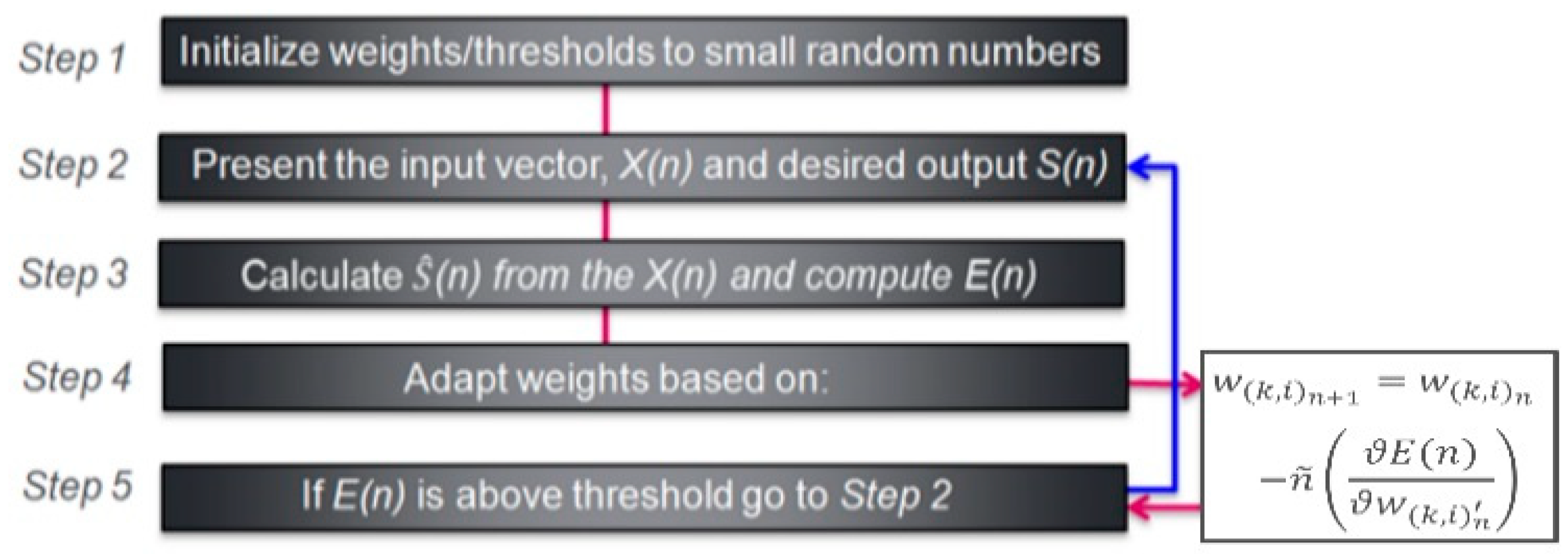
4.1. Artificial Neural Network (ANN)

An ANN-NLE based on the multilayer perceptron (MLP) has been implemented in [21]. MLP-ANNs form a complex map with non-linear decision boundaries between input and output spaces, helping in inverting the effects of non-linear distortion. ANN is an emerging technology applied in contemporary wireless communications for the reduction of OFDM-based non-linear distortion in power amplifiers. ANN schematic diagram for m-QAM CO-OFDM is shown in Figure 3b, which is placed directly after the fast Fourier transform (FFT) at the digital part of the CO-OFDM receiver (see Figure 3a). In summary, it comprises of p sub-neural networks considering a single hidden-layer. Each sub-network is being associated to each subcarrier k, and where s(k) is the training vector. The received symbols, i, for each subcarrier x{k} are processed by the ANN neurons which are subsequently multiplied with a weight value, w_k,i, for each subcarrier where the outputs of all subcarriers are summed. In the training stage, the minimum mean-square error (MMSE) algorithm determines the error signal and updates the weights, which are iteratively updated until the desired error value is reached, thus indicating the optimal match between the sub-network output and the transmitted CO-OFDM symbols. The error signal is given as $E\left(k\right)=s\left(k\right)-\widehat{s}\left(k\right),$ where ŝ(k) is calculated in terms of a non-linear activation function (NAF), φ_k,i, that is given by $\widehat{s}\left(k\right)={\displaystyle \sum }_{i=1}^M{w}_{k,i}{\phi }_{k,i}\left(s\left(k\right)\right)$. The chosen NAF is a differential sigmoid function and is a “split” complex NAF, where two conventional real-valued functions process the I-Q components in contrast to our proposed approach which processes the complex data simultaneously, thus accounting for real and imaginary data cross-information. The number of ANN neurons in every sub-neural network is equal to the number of points of the constellation. The 2D ANN is based on the Riedmiller’s resilient-back propagation (RR-BP) algorithm and performs an approximation to the global minimization achieved by the steepest descent [20]. The training function updates the weights and bias values according to RR-BP, which minimizes the difference between the ANN output and the desired output by splitting the complex OFDM data in two real-valued data collections. The transfer functions for the hidden layer of the ANN are differentiable and similar to the hyperbolic tangent function. For the output layer, the linear function “purelin” was employed [20]. The MMSE in Figure 3a represents the subsystem that implements RR-BP to find the weights that minimize the error vector $E\left(n\right)=\parallel S\left(n\right)-\widehat{S}\left(n\right){\parallel }^2$, where $S\left(n\right)$ and $\widehat{S}\left(n\right)$ are the desired and calculated output vectors, respectively. The weights are updated according to the steps described in Figure 4 by applying the gradient descent on the cost function E(n) to reach a minimum. Finally, at the end-output of Figure 3b we introduced slack variables that allow some misclassified symbols but penalizes them.

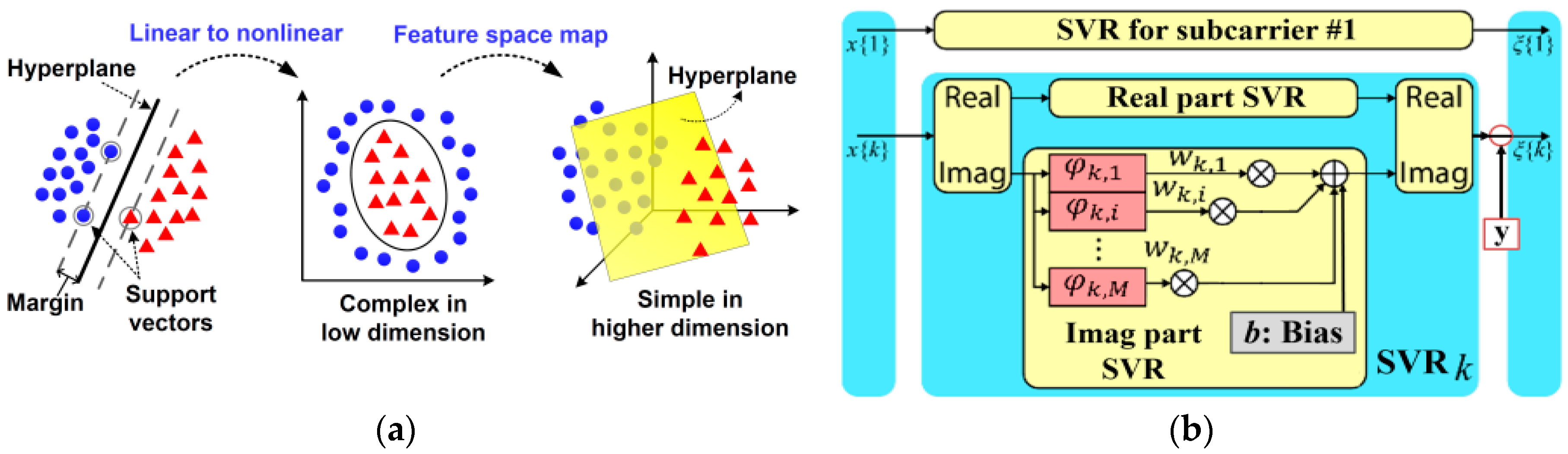
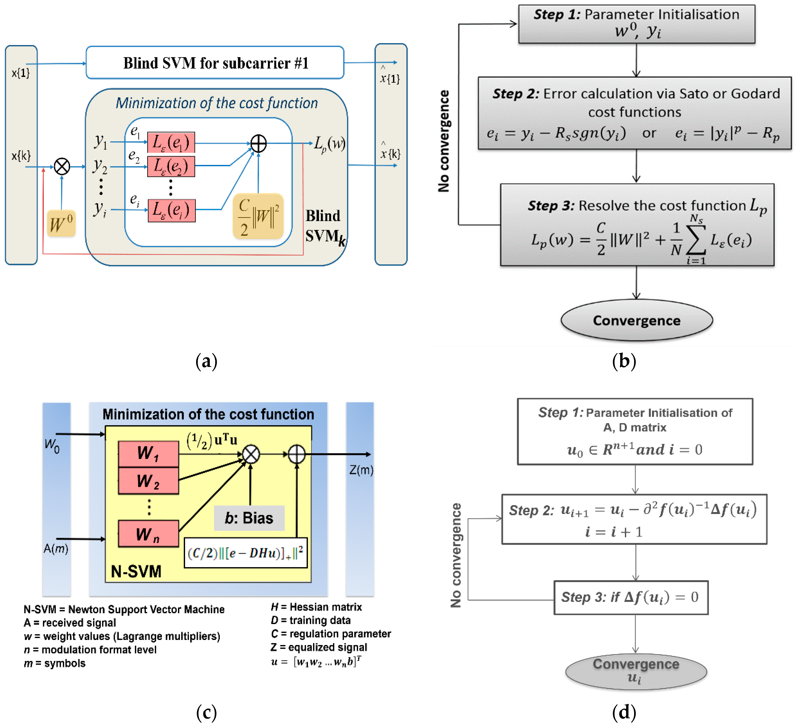
4.2. Support Vector Machine (SVM)

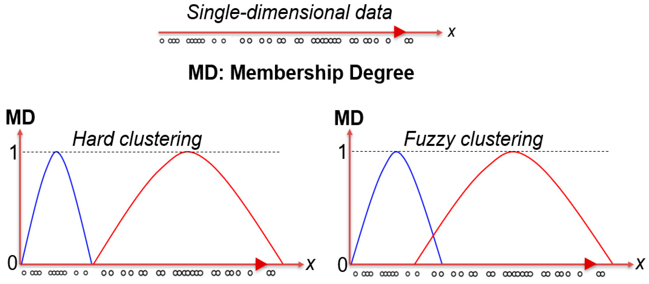
The SVM is placed in the same NLE block as in Figure 3a. In Figure 5b the supervised support vector regressor (SVR)-NLE is shown [28,30], which in contrast to other versions such as in [27] that only classifies the data (i.e., support vector classifier, SVC), SVR is considered more advanced as it performs both classification and regression and for simplicity is called SVR. It is comprised of k hidden nodes (support vectors), with each node being associated to each subcarrier k. The procedure of SVR is similar to [28,30]. In summary, the received symbols for each subcarrier x{k} are processed by the NLE supported vectors which are scaled by weight values (Lagrange multipliers) for each subcarrier w_k,i, after which, the outputs for different k are summed. The distribution of noisy constellation points is learnt during an initial training process similarly to ANN. Once the distribution is learnt, the detector can make decision for the new unknown observation symbols. A hyperplane is also obtained through approximation of a nonlinear function using a set of Kernels (sigmoid function) of training dataset. SVR maps the data to a high-dimension feature space as shown in Figure 5a, using a nonlinear mapping φ and then linear regression is formulated by introducing the “ε-insensitive” loss function in the following form $f\left(x,w\right)= {\displaystyle \sum }_{i=1}^M{w}_{k,i}{\phi }_{k,i}\left(x\right)+b,$ where $f\left(x,w\right)$ is the target linear model, ${\phi }_{k,i}\left(x\right)$ denotes a set of nonlinear transformations of input x, and b is the bias term. The number of vectors in every hidden node is equal to the number of points of the constellation; hence for example for 4-QAM is 4. The “ε-insensitive” loss function can be learnt through training process by minimizing the error, $\psi \left(w,\xi \right)=\frac{1}{2}{\parallel w\parallel }^2+C\sum \left({\xi }_k^{-}+{\xi }_k^{+}\right),$ where ${\xi }_k^{-},{\xi }_k^{+}$ are slack variables corresponding to the upper and lower bounds on the output function and C is the penalty parameter. Depending on how much loss is ignored, the latter equation can be approximated by the Lagrange loss function $L\left(y,f\left(x,w\right)\right)$.

It should be indicated that an unsupervised and faster version of SVM was employed in [31,33] and [29], respectively. For the unsupervised SVM, the Sato’s and Godard’s-based constant modulus algorithm (CMA) cost functions were employed in the penalty term of an SVM-like cost function, being iteratively minimized by re-weighted least squares (IRWLS) [23,25]. Figure 6 depicts (a) such SVM algorithm in CO-OFDM for blind-NLE (BNLE) operation, and (b) shows the inherent IRWLS pseudocode. In this algorithm, the received OFDM symbols for each subcarrier x{k} are processed by the BNLE which are scaled by the vector of filter coefficients (weights) for each subcarrier (k) w_k,i (where i is the symbol) by means of a hybrid maximum likelihood and recursive least-square process [25]. In the IRWLS steps, described in Figure 6b, w refers to the weights, y refers to the received symbols (reference sequence), while $L_{\epsilon }\left(e_i\right)$ is the loss function, C a penalty regulation parameter, $e_i$ the penalization term for the ith symbol, and Ns is the total number of subcarriers. Finally, $R_s \mathrm{and}{R}_P$ refer to the Sato’s and Godard’s constants, respectively. For the fast version of SVM, a Newton SVM was implemented with an architecture as shown in Figure 6c. Newton SVM suppresses the input space features for a nonlinear programming formulation of supervised SVM classifiers. This stand-alone method can handle classification problems in very high dimensional spaces. In this algorithm, a Newton-based algorithm is solved which is implemented via Lagrangian multipliers of an SVM-based classifier, thus resulting to an effective iterative scheme [29] constituted of only a few steps. To process a high-level modulation format order (and thus constellation mapper) with a large dimensional input, a fast-finite Newton approach was considered. For the classification problem, this approach searches for a unique Lagrangian-based global minimum solution by determining a finite number of times, a system of nonlinear equations. The aforementioned Newton-based algorithm steps and related equations are depicted in Figure 6d which involves an Armijo step-size [29]. In the equations in Figure 6d, column vectors are considered except if transposed to a row vector (using a $T$ superscript). Moreover, as depicted in Figure 6c, $\parallel x\parallel$ denotes the 2-norm of a vector x, while A is the matrix related to an OFDM received signal incorporating m complex symbols in the n-dimensional real space $R^m$ which expresses the modulation order level (i.e., 4 for 16-QPSK).

4.3. Clustering

In this section, we briefly describe the structure of the four main unsupervised machine learning based clustering algorithms that have been applied in long-haul CO-OFDM as BNLEs, i.e., the K-means, fuzzy-logic C-means (named here as FL or FLC), and affinity propagation (name here as AP) clustering algorithms.

K-means: Is the most common clustering algorithm based on an iterative, data-partitioning process, assigning n observations to exactly one of the k clusters defined by centroids, where k is chosen before the algorithm starts [35]. The algorithm proceeds as follows:

• Choose k initial cluster centers (centroid).
• Compute point-to-cluster-centroid distances of all observations to each centroid.
• Compute the average of the observations in each cluster to obtain k new centroid locations.
• Repeat steps 2 through 3 until cluster assignments do not change, or the maximum number of iterations is reached.

FL: This belongs to the probabilistic machine learning algorithms, and permits the symbols to fluctuate the data membership degree (MD) while being allocated into many clusters as shown in Figure 7 by minimizing the objective function: $F_m={\displaystyle \sum }_{i,j}^N{\displaystyle \sum }_{i=1}^R{\displaystyle \sum }_{j=1}^L{\mu }_{ij}^m\parallel t_i-c_j\parallel {}^2.$ In this objective function, the terms m, L, N, and R, correspond to the “Fuzzy partition matrix exponent”, clusters, total number of subcarriers and symbols, respectively. The role of the “Fuzzy partition matrix exponent” is to adjust the grade of overlapping between clusters. Where t_i is referred to the ith symbol, c_j is the center of a jth cluster, and μ_ij refers to the MD of t_i into jth cluster. FL is processed in 5 steps: 1. Enter the number of targeted clusters; 2. Initiate the cluster MD, μ_ij; 3. Estimate the center per cluster by $C_j={\displaystyle \sum }_{i,j}^N({\displaystyle \sum }_{i=1}^R{\mu }_{ij}^m{X}_i/{\displaystyle \sum }_{i=1}^R{\mu }_{ij}^m)$; 4. Update μ_ij using $C_j=1/{({\displaystyle \sum }_{i,j}^N{\displaystyle \sum }_{k=1}^L\parallel t_i-c_J\parallel /\parallel t_i-c_k\parallel )}^{2/m-1}$ and compute F_m; 5. Return and perform steps 2–4 until F_m is converged at a desired threshold.

AP: Every symbol in AP is a potential exemplar by viewing each symbol as a node that recursively transmits real-valued messages (separately for amplitude and phase) along the edges of the NLE network until a good set of exemplars and corresponding clusters emerges [36]. ‘Messages’ are updated by simple formulas that search for minima of an appropriately chosen energy function. At any symbol in time the magnitude of each message reflects the current affinity that 1 symbol has for choosing another symbol as its exemplar. Let x₁ through x_n be a set of complex data (symbol), with no assumptions made about their internal structure, and let S be a function that quantifies the similarity between any 2 symbols, such that S(x_i, x_j)>S(x_i, x_k) if x_i is more similar to x_j than to x_k. For this example, the negative squared distance of 2 symbols was used i.e., for points x_i and x_k,

$s\left(i,k\right)=-\parallel x_i-x_k\parallel {}^2$. The diagonal of S (i.e., S(i,i)) is particularly important, as it represents the input preference, meaning how likely a particular input is to become an exemplar. When this is set to the same value for all inputs, it controls how many classes the algorithm can produce. A value close to the minimum possible similarity produces fewer classes, however, a value close or larger to the maximum possible similarity, produces many classes (initialized to the median similarity of all pairs of inputs). AP proceeds by alternating 2 message passing steps to update the ‘responsibility, R(i, k)’ and ‘availability, A(i, k)’ matrices, where R quantifies how “well-suited” x_k is to serve as the exemplar for x_i compared to other candidate exemplars, while A shows how “appropriate” it would be for x_i to pick x_k as its exemplar, taking into account other points’ preference. R and A, are initialized to zero being viewed as log-probability tables and then AP is iteratively updated for R and A by:

$$\begin{gathered} R\left(i,k\right)=s\left(i,k\right)-{\max }_{k^{\prime }\ne k}\left\{a\left(i,k^{\prime }\right)+s\left(i,k^{\prime }\right)\right\} \\ A\left(i,k\right)=\min {\left(0,r\left(k,k\right)+{\displaystyle \sum }_{i^{\prime }\ne \left\{i,k\right\}}\max (0,r\left(i^{\prime },k\right)\right)}_{\mathrm{for}i\ne k} \end{gathered}$$

The exemplars are extracted from the final updated matrices where ‘responsibility + availability’ is positive. Figure 8 shows the AP iterative result of R and A for a QPSK middle-channel in WDM CO-OFDM at 3200 km for an optimum launched optical power (LOP) per channel of –5 dBm, where 13 iterations are required for convergence [36]. AP is considered as an advanced soft-clustering algorithm.

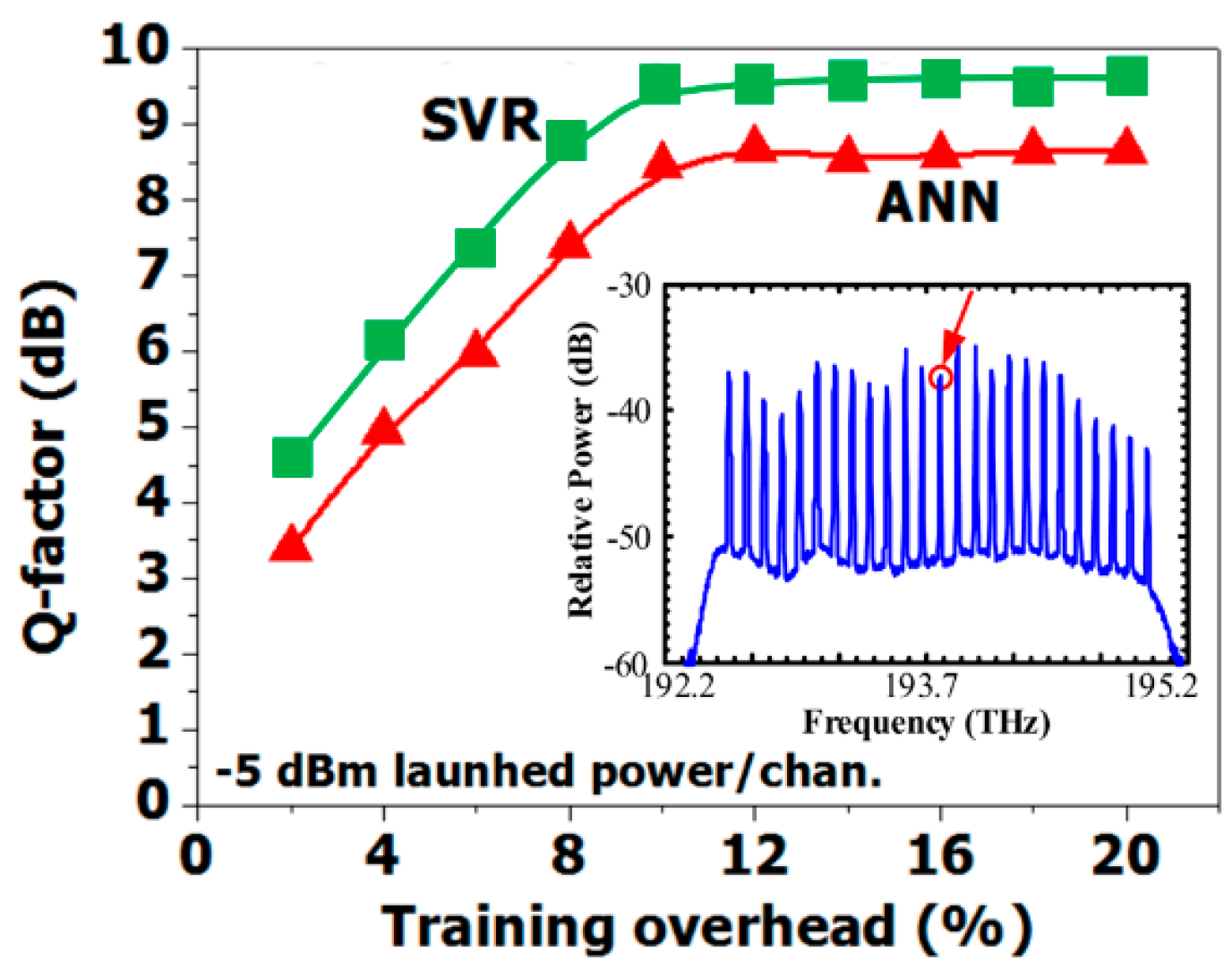
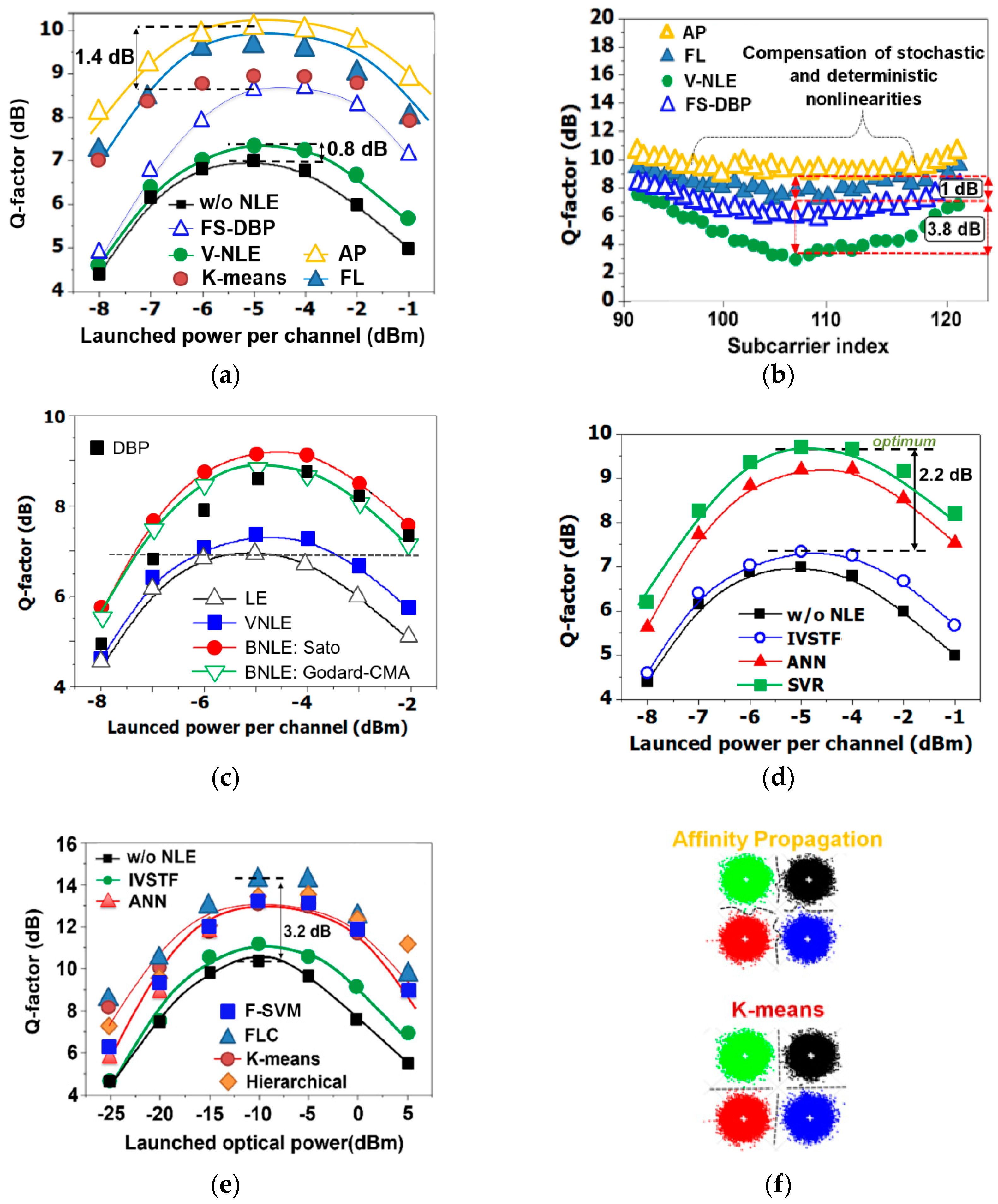
5. Experimental Setup and Performance of Machine Learning Algorithm in CO-OFDM

The experimental setup and parameters are shown in Figure 9 and

Table 1. Transmission and transceiver OFDM parameters.

Parameter	Value
Net bit-rate	18.2 Gb/s(WDM), 40 Gb/s(1-ch.)
Net bit-rate for ANN	16.8 Gb/s (WDM), 38 Gb/s(1-c.)
Raw bit-rate	20 Gb/s (WDM), 46 Gb/s (1-ch.)
Format of modulation	QPSK (WDM), 16-QAM (1-ch.)
Number of symbols	400
Symbol time duration	20.48 ns
Generated subcarriers	210
CP	2%
Size of FFT & inverse(I)FFT	512
ANN Training overhead	10%
ANN Train. symbol length	40 symbols
Local oscillator linewidth	100 kHz
OH-LITE fiber attenuation	18.9–19.5 dB/100km
Number of spans	30 (WDM), 20 (1-chan.)
Length-per-span	100 km
Center wavelength	1550.2 nm

for both single-channel and WDM CO-OFDM at 2000 km and 3200 km of transmission, respectively, using EDFA-based recirculating loops and a standard single-mode fiber (SSMF). The set-up, procedures and parameters are identical to [21,22,28,31,33,35,36]. In summary, 400 OFDM symbols (20.48 ns length) were generated using a 512-point IFFT on 210 QPSK/16-QAM subcarriers. To eliminate inter-symbol-interference from linear effects, a cyclic prefix (CP) of 2% was included. For the clustering algorithms, FS-DBP, V-NLE and without (w/o) NLE, the raw bit-rates were ~20 Gb/s (QPSK) and 40 Gb/s (16-QAM). However, for supervised machine learning such as SVR and ANN (as indicated in Table 1), 10% of data are sacrificed for training for both single- and multi-channel cases, above which the quality(Q)-factor is saturated as depicted in Figure 10 for WDM CO-OFDM. Such training is performed separately for each LOP, requiring relatively the same amount of training-data. At the receiver side, a coherent optical homodyne receiver was used, while the offline OFDM demodulator included timing synchronization, frequency offset compensation (due to the receiver local oscillator, LO), channel estimation and equalization with the help of an initial training sequence, as well as IQ imbalance and CD compensation using an overlapped frequency domain equalizer. For the WDM CO-OFDM system a laser grid of 100 kHz-linewidth distributed feedback lasers (DFBs) on 100 GHz grid was used and the noise loading channels were inserted using ASE source and a wavelength selective switch (WSS). In the inset spectrum of Figure 10 (as well as in the inset of Figure 9) the received WDM lines are shown. The NLEs performances were assessed by the total subcarriers’ bit-error-rate (BER) and Q-factor (=20log₁₀$\left[\sqrt{2}erf{c}^{-1}\left(2BER\right)\right])$) measurements averaging over 10 recorded traces (~10⁶ bits) by error counting (hard-decision-decoding, HDD).

In Figure 11, the Q-factor against the LOP per channel is plotted for various machine learning and deterministic NLEs for the QPSK middle-channel in WDM CO-OFDM. It shown that AP tackles non-linearities more effective than any other algorithm under test since it compensates both the PNA and the accumulated inter-subcarrier FWM which appears random (due to the impact of a high PAPR). This is corroborated in Figure 11b, where the Q-factor for the middle subcarriers is plotted which suffers the most mainly from inter-subcarrier FWM [48] (secondary from inter-subcarrier cross-phase modulation, XPM) at the optimum LOP. However, some of the inter-channel nonlinearities are also compensated better by AP, which are not as strong as the intra-channel (i.e., inter-subcarrier nonlinear distortions). In Figure 11f, the clear nonlinear decisions (soft/overlapping clustering) compared to K-means hard decisions (exclusive clustering) is also depicted for a received QPSK constellation diagram at −7 dBm of LOP. In Figure 11c–e we show the performance of unsupervised, supervised and fast machine learning algorithms, i.e., Sato/Godard-CMA BNLEs, ANN/SVR, and Fast-Newton-SVM (F-SVM), respectively. Results in Figure 11c–e conclude that AP clustering algorithm has the best performance in QPSK WDM CO-OFDM, and then SVR and FL follow. Finally, in Figure 11 it is shown that at low power a Q-factor improvement of the adopted machine learning algorithms is observed over the deterministic algorithms and linear equalization. This is due to the ability of machine learning NLEs to partially tackle the accumulated ASE noise from concatenated optical amplifiers. Such statement is strong considering the negligible noise induced from electrical components and digital-to-analogue and analogue-and-digital converters (error vector magnitude below 7% for optical back-to-back).

In Figure 12, results are depicted for single-channel 16-QAM CO-OFDM using the same algorithms. Similarly, AP shows the greatest performance reaching almost 15 dB in Q-factor and outperforming the FS-DBP. This means that the strong nonlinear phase noise of 16-QAM can be successfully tackled by AP, which seems to effectively compensating intra-channel deterministic and stochastic nonlinearities. However, it should be noted that all algorithms at low powers present poor performance due to the stronger PNA and ASE noise. It should be noted that an ANN was also implemented in [20,21], however, the bit-rate and training testing was different than SVR and so is not included here to be compared. Nevertheless, as shown in [20,21] the performance is anticipated to be worse than SVR and consequently and from AP.

6. Complexity Analysis

In order to evaluate and compare the complexity of the different NLEs under test, we should first note that the nature of the deterministic equalizers based on DBP and IVSTF is essentially different from machine learning-based NLEs such as ANN and SVM. On the one hand, since DBP and IVSTF equalizers require an inversion of the propagation model, they are dependent on several link and bandwidth parameters. In particular, they depend on the number of spans of the oversampling parameter and, in the case of DBP, on the chosen spatial step. The complexity of these equalizers, though, does not depend a priori on other signal parameters such as modulation format. Machine learning based NLEs, on the contrary, present a complexity that does not depend on the link parameters but on some signal parameters, for instance the number of constellation points and the number of OFDM subcarriers. Hence, the computation of the complexity of each NLE family requires special attention. The following subsections deal with the complexity analysis of deterministic and machine learning approaches. In addition, we shall discuss the complexity of some clustering algorithms. For the sake of clarity in the derivation of the complexity expressions, the following table lists the employed parameters and their associated variable names (

Table 2. Parameters employed in the calculation of complexity.

Link parameters		Signal parameters
Symbol	Definition	Symbol	Definition
Nspan	Number of spans	NSC	Subcarrier number
Lspan	Length per span	K	Oversampling factor
Δd	Spatial step	M	No. bits per subcarrier

). We shall consider the number of operations to process an OFDM symbol. Hence, in order to obtain the number of operation-per-bit, the number of operations should be divided by the number of bits per OFDM symbol.

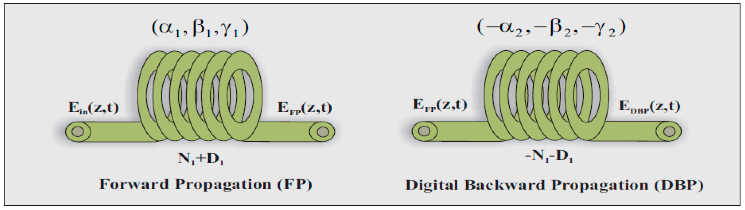
6.1. Complexity Analysis of Digital Back-Propagation (DBP) and Inverse-Volterra Series-Transfer Function (IVSTF)-Based Non-Linear Equalizations (NLEs)

Both DBP and IVSTF based NLEs can be implemented fully in the time domain, frequency domain, or in the hybrid time-frequency domain [13]. In this work, we assume the latter, as this is a commonly adopted approach in either DBP- or IVSTF-based NLEs. As indicated in previous section, in the case of DBP, the most widely employed method is the SSF with inverted parameter values. In this method, the CD is simulated in the frequency domain whereas the non-linear Kerr effect is simulated in the time domain. On the other hand, the IVSTF NLEs implemented in the hybrid time-frequency domain make use of the simpler calculation of high dimensional convolution in the frequency domain. Both methods, therefore, require multiple conversion from the frequency domain to the time domain and vice versa. This conversion is performed using FFT/IFFT pairs that operate on data blocks of size N_block = K·N_signal, since the data has to be oversampled with an oversampling constant K in order to account for the out-of-band non-linear components. When the N_block is a power of two, the split-radix is the implementation showing the lowest complexity [13] requiring the floating-point (FLOPs) real-valued operations from (1):

$$N_{FFT}=N_{IFFT}=4N_{block}{\log }_2{N}_{block}-6N_{block}+8$$

(1)

6.1.1. Complexity of NLEs Based on Digital Back-Propagation

Each DBP segment requires a time-to-frequency and a frequency-to-time conversion, in addition to the operations to implement both the non-linear and linear compensation stages. The number of FLOPs for each DBP steps is then:

$$N_{step}=N_{linear}+N_{nonlinear},$$

(2)

where N_linear and N_non-linear are given by 8N_block log₂N_block −6N_block + 16 and 18N_block, respectively. On the other hand, the number of DBP steps is, assuming uniform length:

$$N_{steps }= \frac{N_{spans}\times L_{span}}{\Delta d}.$$

(3)

The total number of FLOPs required by the DBP is then given by

$$\begin{gathered} N_{DBP }= \frac{N_{spans}\times L_{span}}{\Delta d}(N_{linear}+N_{nonlinear}) \\ = \frac{N_{spans}\times L_{span}}{\Delta d}(8{N_{\mathrm{block}}}_{}{\log }_2{N}_{\mathrm{block}}+12N_{\mathrm{block}}+16) \end{gathered}$$

(4)

6.1.2. Complexity of NLEs Based on Inverse Volterra Series Transfer Function (IVSTF)

The procedure to calculate the number of FLOPs required by the IVSTF-based NLE is similar to that of DBP-based NLE since multiples time-to-frequency and frequency-to-time conversions are required. The number of operations, however, does not depend on the link spatial discretization but on the number of links. Looking at the blocking diagram of Figure 2, we can observe, that IVSTF-based NLE requires a linear compensation block and a non-linear equalization block per span, that is, N_span, and therefore, the total number of FLOPs can be calculated as:

$$N_{IVSTF}=N_{linear}+N_{span}\times N_{nonlinear}$$

(5)

Here, N_linear is given by:

$$N_{linear}=N_{FFT}+N_{prod}+N_{IFFT},$$

(6)

where N_prod is the number of operations for linear equalization, which is given by 6N_block as it requires N_block complex multiplications (6FLOPs each). The number of FLOPs for the non-linear compensation block, on the other hand, is:

$$N_{nonlinear}=N_{prod}+N_{IFFT}+N_{square}+2N_{prod}+N_{FFT}+N_{prod}.$$

(7)

The square operation can be seen as an element-by-element multiplication of N_blocks data and, consequently, also requires 6N_blocks. Consequently, the total number of operations for the IVSTF-based NLE is given by:

$$N_{IVSTF}=\left(N_{span}+ 1\right)8N_{block}{\log }_2{N}_{block}+\left(20N_{span}-6 \right)N_{block}+16\left(N_{span}+1\right)$$

(8)

6.2. Complexity Analysis of ANN and SVM-Based NLEs

As mentioned, in contrast to DBP and IVSTF-based equalizers, the complexity of ANN and SVM-based equalizers depends on the parameters of the modulation format. In the particular case of OFDM, it depends on the number of data subcarriers (N_SC) and the number of bits coded in each subcarrier (M).

6.2.1. Complexity of ANN

ANNs mimic natural neural systems making use of massive parallel low-complexity nodes. Therefore, it is not a surprise that their implementation requires fewer FLOPs than other approaches. After learning, and assuming that the non-linear activation function is implemented using a look-up table, the number of operations performed for processing each OFDM symbol can be obtained by,

$$N_{ANN}=2\left[M\left(M-1\right)\right]N_{SC}.$$

(9)

6.2.2. Complexity of SVM

In order to calculate the complexity of implementing the SVM-NLE, we can split the equalization process in two steps. On the one hand, the process of estimating the ML-RLS, whose complexity does not depend whether the equalization is blind. On the other hand, the complexity of performing the IRWLS that depends on the equalization type, i.e., blind or non-blind, and on the chosen cost function, in our case Sato’s or Godard’s cost function. We consider that the NLE algorithm operates using a N_w order filter operating on data blocks of Ns samples. The complexity of each iteration within the ML-RLS estimation can be calculated step by step. The first step that is the computation of a_i is given by 8N_W + 3. The second step, where the w_s is calculated using the least-square method, requires 64/3N_s³ + 18N_s². The updating of the w vector carried out in the third step depends on particular implementation. For the case of the supervised SVM, the number of operations is 4N_w + 6N_s −1, whereas for Sato’s and Godard’s based blind implementations, the number operations is 3N_s² + 2N_s and (3p + 2)N_s² + (p + 2)N_s (p represents the power of the norm), respectively. Step four and step five a priori do not affect the FLOP count since they do not require any extra arithmetic manipulation. It is important to note that in all the studied cases, the computational complexity is O($N_S^3$), with the least square calculation the limiting stage. The computational complexity of the cost function, on the other hand, is O(N_s) for non-blind equalization and O($N_S^2$) for both Sato’s and Godard’s cost functions and, consequently, blind equalization does not suppose a significant computational cost increment compared to the unsupervised approach.

6.3. Complexity of Clustering Algorithms

The complexity of the clustering algorithms is dependent on how many clusters can be found. Since in most cases each cluster corresponds to a constellation point, the complexity will depend on the modulation format. However, in contrast to ANN, the complexity of the clustering algorithms is also dependent on the number of samples employed for clustering and their dispersion, which significantly impacts the convergence of the algorithm. Therefore, it is not possible to deterministically compute the number of required operations. A commonly adopted criterion is the worst-case scenario that represent a pessimistic upper bound to the complexity.

6.3.1. K-means

For K-means clustering, the number of operations in the worst-case-scenario if the Lloyd’s algorithm is used is given by O(nkdi), where n is the number of data to be clustered, k is the number of clusters (2^M), d is the dimensionality (in our case, 2), and i = 2^Ω(√n) is the number of the required iterations.

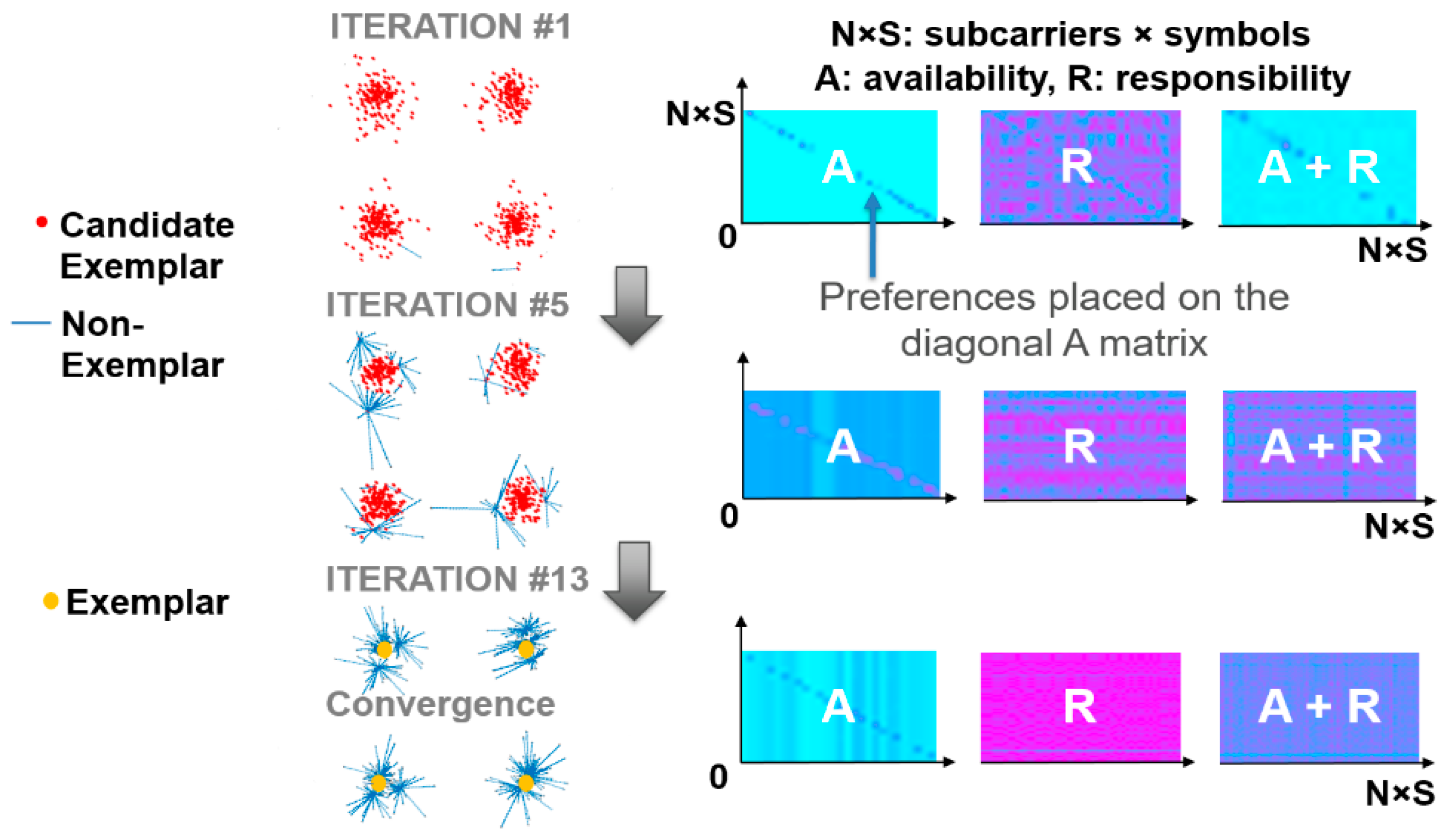
6.3.2. Affinity Propagation

In the case of AP, the number of operations is O(ikn²), where i, k and n are the number of iterations, clusters, and elements, respectively. While the number of clusters and element are trivial, the number of iterations i is difficult to predict due to the complexity algorithm and its interplay with the dispersion structure of the data.

6.4. Impact of High-Order Modulation Format Levels on Computational Complexity

In this section, we investigate the impact of high-order modulations formats (up to 128-QAM) on the computational complexity of the most widely-adopted machine learning, ANN. We also provide a comparison in

Table 3. Computational complexity comparison between full-step DBP, IVSTF and ANN for different modulation format order (M) and transmission distances.

Deterministic Technique	System A (2000 km)	System B (3200 km)
DBP	163852800 (1.6 × 108)	262164480 (2.6 × 108)
IVSTF	1151312 (1.2 × 106)	1839632 (1.8 × 106)
ANN (M = 4)	5040 (5.0 × 103)
ANN (M = 16)	100800 (1.0 × 105)
ANN (M = 64)	1693440 (1.7 × 106)
ANN (M = 128)	6827520 (6.8 × 106)

between full-step DBP, IVSTF and ANN, for two systems with different total lengths and different numbers of constellation points. Since the ANN is independent of the link parameters, the ANN complexity is the same for both systems. From Table 3, it is evident that DBP is the technique with the highest computational complexity compared to ANN for both low- and high-modulation format levels. However, when comparing IVSTF with ANN for large constellation point numbers, it can be appreciated that for the System A (transmission at 2000 km) IVSTF has lower complexity than ANN for M = 64 and above, while for System B (transmission at 3200 km) IVSTF has lower complexity than ANN only for M = 128. We note that we made the calculations assuming 40 steps-per-span for the full-step DBP. With regard to the subcarrier numbers, we considered 512 for IVSTF and DBP (as this is used to calculate the total occupied band) and 210 for the ANN (because subcarriers carrying data are only processed by the NLEs).

7. Conclusions

We reviewed the most commonly used machine learning algorithms for receiver-based NLE in CO-OFDM that include both unsupervised and supervised algorithmic designs for blind and non-blind NLE processing, respectively. We identified the main sources of noise in a coherent fiber-optic telecommunication system and analyzed the limitations of benchmark deterministic solutions (e.g., MS-OPC, PCSC, DBP), highlighting that their prominent obstacle is the inability of tackling stochastic non-linear distortions in long-haul CO-OFDM such as the PNA effect. We showed the performance of machine learning-based NLEs over 2000 km and 3200 km of SSMF transmission for a 16-QAM ($~$40 Gb/s) and a QPSK-WDM ($~$20 Gb/s middle-channel) CO-OFDM system, respectively. The machine learning algorithms included clustering algorithms such as K-means (deterministic hard-clustering), FL (probabilistic soft-clustering), AP (advanced soft-clustering); supervised machine learning algorithms such as ANN (classification) and SVR (classification and regression); unsupervised and fast SVMs; and compared with the deterministic benchmark approaches of FS-DBP and IVSTF. We also presented, for the first time, a computational complexity analysis among machine learning and deterministic algorithms. Our review indicated that AP offers the best performance for both 16-QAM and QPSK-WDM CO-OFDM having, however, higher computational complexity with other supervised/unsupervised machine learning algorithms. Machine learning reveals a much lower complexity and a significant performance benefit over deterministic approaches especially for QPSK-WDM due to their ability of tackling both intra- and inter-channel non-linearities (including inter-subcarrier non-linear crosstalk distortions) mainly on middle subcarriers which suffer the most from inter-subcarrier FWM. We believe that due to their impressive performance and low complexity, machine learning algorithms could play a key role in long-haul coherent optical communications.

References

1. Winzer, P.J. Scaling optical fiber networks: Challenges and solutions. Opt. Photonics News 2015, 26, 28–35. [Google Scholar] [CrossRef]
2. Cisco Virtual Networking Index: Forecast and Methodology, 2014–2019; CISCO: San Jose, CA, USA, 2015.
3. Mitra, P.P.; Stark, J.B. Nonlinear limits to the information capacity of optical fiber communications. Nature 2001, 411, 1027–1030. [Google Scholar] [CrossRef] [PubMed]
4. Agrawal, G.P. Nonlinear Fiber Optics, 3rd ed.; Academic Press: San Diego, CA, USA, 2001; ISBN 0-12-045143-3. [Google Scholar]
5. Temprana, E.; Myslivets, E.; Kuo, B.P.; Liu, L.; Ataie, V.; Alic, N.; Radic, S. Overcoming Kerr-induced capacity limit in optical fiber transmission. Science 2015, 348, 1445–1448. [Google Scholar] [CrossRef] [PubMed]
6. Behrens, C. Mitigation of Nonlinear Impairments for Advance Optical Modulation Formats. Ph.D. Thesis, Department of Electronic and Electrical Engineering, University College London, London, UK, 2012. [Google Scholar]
7. Ellis, A.D.; McCarthy, M.E.; Al Khateeb, M.A.; Sorokina, M.; Doran, N.J. Performance limits in optical communications due to fiber nonlinearity. Adv. Opt. Photonics 2017, 9, 429–503. [Google Scholar] [CrossRef]
8. Shieh, W.; Athaudage, C. Coherent optical orthogonal frequency division multiplexing. Electr. Lett. 2006, 42, 587–589. [Google Scholar] [CrossRef]
9. Morshed, M.; Du, L.B.; Lowery, A.J. Mid-Span Spectral Inversion for Coherent Optical OFDM Systems: Fundamental Limits to Performance. J. Lightw. Technol. 2013, 31, 58–66. [Google Scholar] [CrossRef] [Green Version]
10. Le, S.T.; McCarthy, M.E.; Mac Suibhne, N.; Al-Khateeb, M.A.; Giacoumidis, E.; Doran, N.; Ellis, A.D.; Turitsyn, S.K. Demonstration of Phase-conjugated Subcarrier Coding for Fiber Nonlinearity Compensation in CO-OFDM Transmission. J. Lightw. Technol. 2015, 33, 2206–2212. [Google Scholar] [CrossRef]
11. Gao, G.; Zhang, J.; Gu, W. Analytical Evaluation of Practical DBP-Based Intra-Channel Nonlinearity Compensators. Photonics Technol. Lett. 2013, 25, 717–720. [Google Scholar] [CrossRef]
12. Song, M.; Pincemin, E.; Vgenopoulou, V.; Roudas, I.; Amhoud, E.M.; Jaouën, Y. Transmission performances of 400 Gbps coherent 16-QAM multi-band OFDM adopting nonlinear mitigation techniques. In Proceedings of the 2015 Tyrrhenian International Workshop on Digital Communications TIWDC, Florence, Italy, 22 September 2015; pp. 46–48. [Google Scholar]
13. Giacoumidis, E.; Aldaya, I.; Jarajreh, M.A.; Tsokanos, A.; Le, S.T.; Farjady, F.; Jaouën, Y.; Ellis, A.D.; Doran, N.J. Volterra-Based Reconfigurable Nonlinear Equalizer for Coherent OFDM. Photonics Technol. Lett. 2014, 26, 1383–1386. [Google Scholar] [CrossRef]
14. Yu, Y.; Zhao, J. Modified phase-conjugate twin wave schemes for fiber nonlinearity mitigation. Opt. Exp. 2015, 23, 30399–30413. [Google Scholar] [CrossRef]
15. Yoshida, T.; Sugihara, T.; Ishida, K.; Mizuochi, T. Spectrally-efficient Dual Phase-Conjugate Twin Waves with Orthogonally Multiplexed Quadrature Pulse-shaped Signals. In Proceedings of the Optical Fiber Communication Conference (OFC), San Francisco, CA, USA, 9–13 March 2014. [Google Scholar]
16. Egmont-Petersen, M.; de Ridder, D.; Handels, H. Image processing with neural networks—A review. Pattern Recognit. 2002, 35, 2279–2301. [Google Scholar] [CrossRef]
17. Ye, H.; Li, G.Y.; Juang, B.-H. Power of Deep Learning for Channel Estimation and Signal Detection in OFDM Systems. Wirel. Commun. Lett. 2018, 7, 114–118. [Google Scholar] [CrossRef]
18. Zibar, D.; Wymeersch, H.; Lyubomirsky, I. Machine learning under the spotlight. Nat. Photonics 2017, 11, 751. [Google Scholar] [CrossRef]
19. Argyris, A.; Bueno, J.; Fischer, I. Photonic machine learning implementation for signal recovery in optical communications. Sci. Rep. 2018, 8, 8487. [Google Scholar] [CrossRef] [PubMed] [Green Version]
20. Jarajreh, M.A.; Giacoumidis, E.; Aldaya, I.; Le, S.T.; Tsokanos, A.; Ghassemlooy, Z.; Doran, N.J. Artificial Neural Network Nonlinear Equalizer for Coherent Optical OFDM. Photonics Technol. Lett. 2015, 27, 387–390. [Google Scholar] [CrossRef]
21. Giacoumidis, E.; Le, S.T.; Ghanbarisabagh, M.; McCarthy, M.; Aldaya, I.; Mhatli, S.; Jarajreh, M.A.; Haigh, P.A.; Doran, N.J.; Ellis, A.D.; et al. Fiber Nonlinearity-Induced Penalty Reduction in Coherent Optical OFDM by Artificial Neural Network based Nonlinear Equalization. Opt. Lett. 2015, 40, 5113–5116. [Google Scholar] [CrossRef] [PubMed]
22. Giacoumidis, E.; Mhatli, S.; Wei, J.; Le, S.T.; Aldaya, I.; Stephens, M.F.; McCarthy, M.E.; Ellis, A.D.; Doran, N.J.; Eggleton, B.J. Intra and inter-channel nonlinearity compensation in WDM coherent optical OFDM using artificial neural network based nonlinear equalization. In Proceedings of the Optical Fiber Communications Conference and Exhibition (OFC), Los Angeles, CA, USA, 19–23 March 2017. [Google Scholar]
23. Koike-Akino, T.; Millar, D.S.; Parsons, K.; Kojima, K. Nonlinearity Equalization with Multi-Label Deep Learning Scalable to High-Order DP-QAM. In Proceedings of the Signal Processing in Photonic Communications (SPPCom), Zurich, Switzerland, 2–5 July 2018. [Google Scholar]
24. Kaur, G.; Kaur, G. Performance analysis of Wilcoxon-based machine learning nonlinear equalizers for coherent optical OFDM. Opt. Quant. Electr. 2018, 50, 256. [Google Scholar] [CrossRef]
25. Kaur, G.; Kaur, G. Application of functional link artificial neural network for mitigating nonlinear effects in coherent optical OFDM. Opt. Quant. Electr. 2017, 49, 227. [Google Scholar] [CrossRef]
26. Ahmad, S.T.; Kumar, K.P. Radial Basis Function Neural Network Nonlinear Equalizer for 16-QAM Coherent Optical OFDM. Photonics Technol. Lett. 2016, 28, 2507–2510. [Google Scholar] [CrossRef]
27. Nguyen, T.; Mhatli, S.; Giacoumidis, E.; Van Compernolle, L.; Wuilpart, M.; Mégret, P. Fiber nonlinearity equalizer based on support vector classification for coherent optical OFDM. Photonics J. 2016, 8, 1–9. [Google Scholar] [CrossRef]
28. Giacoumidis, E.; Mhatli, S.; Nguyen, T.; Le, S.T.; Aldaya, I.; McCarthy, M.E.; Ellis, A.D.; Eggleton, B.J. Comparison of DSP-based nonlinear equalizers for intra-channel nonlinearity compensation in coherent optical OFDM. Opt. Lett. 2016, 41, 2509–2512. [Google Scholar] [CrossRef] [PubMed]
29. Giacoumidis, E.; Mhatli, S.; Stephens, M.F.; Tsokanos, A.; Wei, J.; McCarthy, M.E.; Doran, N.J.; Ellis, A.D. Reduction of Nonlinear Inter-Subcarrier Intermixing in Coherent Optical OFDM by a Fast Newton-based Support Vector Machine Nonlinear Equalizer. J. Lightw. Technol. 2017, 35, 2391–2397. [Google Scholar] [CrossRef]
30. Giacoumidis, E.; Le, S.T.; MacCarthy, M.E.; Ellis, A.D.; Eggleton, B.J. Record Intrachannel Nonlinearity Reduction in 40-Gb/s 16QAM Coherent Optical OFDM using Support Vector Machine based Equalization. In Proceedings of the ANZCOP/ACOFT, Adelaide, Australia, 29 November–3 December 2015. [Google Scholar]
31. Giacoumidis, E.; Mhatli, S.; Le, S.T.; Aldaya, I.; McCarthy, M.E.; Ellis, A.D.; Eggleton, B.J. Nonlinear Blind Equalization for 16-QAM Coherent Optical OFDM using Support Vector Machines. In Proceedings of the ECOC, Düsseldorf, Germany, 18–22 September 2016; p. Th.2.P2. [Google Scholar]
32. Mhatli, S.; Mrabet, H.; Dayoub, I.; Giacoumidis, E. A novel SVM robust model Based Electrical Equalizer for CO-OFDM Systems. IET Commun. 2017, 11, 1091–1096. [Google Scholar] [CrossRef]
33. Giacoumidis, E.; Tsokanos, A.; Ghanbarisabagh, M.; Mhatli, S.; Barry, L.P. Unsupervised Support Vector Machines for Nonlinear Blind Equalization in CO-OFDM. Photonics Technol. Lett. 2018, 30, 1091–1094. [Google Scholar] [CrossRef]
34. Jarajreh, M.A. Compensation of filter cascading effects and non-linearities in flexible multi-carrier-based optical networks using a complex-kernel-based support vector machine. IET Commun. 2018, 12, 1737–1742. [Google Scholar] [CrossRef]
35. Giacoumidis, E.; Matin, A.; Wei, J.; Doran, N.J.; Barry, L.P.; Wang, X. Blind Nonlinearity Equalization by Machine Learning based Clustering for Single- and Multi-Channel Coherent Optical OFDM. J. Lightw. Technol. 2018, 36, 721–727. [Google Scholar] [CrossRef]
36. Giacoumidis, E.; Aldaya, I.; Wei, J.L.; Sanchez, C.; Mrabet, H.; Barry, L.P. Affinity propagation clustering for blind nonlinearity compensation in coherent optical OFDM. In Proceedings of the CLEO, San Jose, CA, USA, 13–18 May 2018. [Google Scholar]
37. Ellis, A.D.; Al Khateeb, M.A.Z.; McCarthy, M.E. Impact of Optical Phase Conjugation on the Nonlinear Shannon Limit. Opt. Exp. 2017, 35, 792–798. [Google Scholar] [CrossRef] [Green Version]
38. Ellis, A.D.; McCarthy, M.E.; Al-Khateeb, M.A.Z.; Sygletos, S. Capacity limits of systems employing multiple optical phase conjugators. Opt. Exp. 2015, 23, 20381–20393. [Google Scholar] [CrossRef]
39. Phillips, I.; Tan, M.; Stephens, M.F.; McCarthy, M.; Giacoumidis, E.; Sygletos, S.; Rosa, P.; Fabbri, S.; Le, S.T.; Kanesan, T.; et al. Exceeding the Nonlinear-Shannon Limit using Raman Laser Based Amplification and Optical Phase Conjugation. In Proceedings of the Optical Fiber Communication Conference (OFC), San Francisco, CA, USA, 9–13 March 2014. [Google Scholar]
40. Sanchez, C.; Mccarthy, M.; Ellis, A.D.; Wright, P.; Lord, A. Optical-phase conjugation nonlinearity compensation in Flexi-Grid optical networks. In Proceedings of the DNCOCO, Budapest, Hungary, 12–14 December 2015; pp. 39–43. [Google Scholar]
41. Liu, X.; Chraplyvy, A.R.; Winzer, P.J.; Tkach, R.W.; Chandrasekhar, S. Phase-conjugated twin waves for communication beyond the Kerr nonlinearity limit. Nat. Photonics 2013, 7, 560–568. [Google Scholar] [CrossRef]
42. Le, S.T.; McCarthy, M.E.; Mac Suibhne, N.; Ellis, A.D.; Turitsyn, S.K. Phase-Conjugated Pilots for Fiber Nonlinearity Compensation in CO-OFDM Transmission. J. Lightw. Technol. 2015, 33, 1308–1314. [Google Scholar] [CrossRef]
43. Czegledi, C.B.; Liga, G.; Lavery, D.; Karlsson, M.; Agrell, E.; Savory, S.J.; Bayvel, P. Digital backpropagation accounting for polarization-mode dispersion. Opt. Exp. 2017, 25, 1903–1915. [Google Scholar] [CrossRef] [PubMed]
44. Irukulapati, N.V.; Wymeersch, H.; Johannisson, P.; Agrell, E. Stochastic digital backpropagation. Trans. Commun. 2014, 62, 3956–3968. [Google Scholar] [CrossRef]
45. Vgenopoulou, V.; Erkilinc, M.S.; Killey, R.I.; Jaouën, Y.; Roudas, I.; Tomkos, I. Comparison of Multi-Channel Nonlinear Equalization using Inverse Volterra Series versus Digital Backpropagation in 400 Gb/s Coherent Superchannel. In Proceedings of the 42nd European Conference on Optical Communication (ECOC), Dusseldorf, Germany, 18–22 September 2016. [Google Scholar]
46. Matsumoto, M.; Nishimura, T. Mersenne Twister: A 623-Dimensionally Equidistributed Uniform Pseudorandom Number Generator. ACM Trans. Model. Comput. Simul. 1998, 8, 3–30. [Google Scholar] [CrossRef]
47. Eriksson, T.A.; Buelow, H.; Leven, A. Applying Neural Networks in Optical Communication Systems: Possible Pitfalls. Photonics Technol. Lett. 2017, 29, 2091–2094. [Google Scholar] [CrossRef] [Green Version]
48. Mateo, E.; Zhu, Z.; Li, G. Impact of XPM and FWM on the digital implementation of impairment compensation for WDM transmission using backward propagation. Opt. Exp. 2008, 16, 16124–16137. [Google Scholar] [CrossRef]
Figure 1. Digital back-propagation (DBP) conceptual diagram [11].
Futureinternet 11 00002 g001
Figure 2. Inverse-Volterra series-transfer function (IVSTF) block diagram for coherent optical orthogonal frequency division multiplexing (CO-OFDM). Where m is the number of spans in a long-haul network and k is the Kernel order [13]. (I)FFT: (Inverse) fast Fourier transform.
Futureinternet 11 00002 g002
Figure 3. (a) CO-OFDM receiver including non-linear equalization (NLE). (b) Artificial neural network (ANN)-NLE. MMSE: minimum-mean square-error [21,22].
Futureinternet 11 00002 g003
Figure 4. Steps required in the ANN training process [17,18].
Futureinternet 11 00002 g004
Figure 5. (a) CO-OFDM receiver including NLE. (b) ANN-NLE. MMSE: minimum-mean square-error [20].
Futureinternet 11 00002 g005
Figure 6. Blind support vector machines (SVMs) (BNLEs): (a) Sato/Godard SVM for CO-OFDM and (b) its iteratively minimized by re-weighted least squares (IRWLS) pseudocode [31,33]; (c) Newton-based SVM and (d) the algorithm’s steps [29].
Futureinternet 11 00002 g006
Figure 7. Conceptual dendrogram for fuzzy-logic (FL) [35].
Futureinternet 11 00002 g007
Figure 8. Affinity propagation (AP) clustering procedure (e.g., quaternary phase-shift keying (QPSK)) [36].
Futureinternet 11 00002 g008
Figure 9. Experimental setup for multi- (upper) and single-channel (lower) CO-OFDM incorporating Volterra-non-linear equalization (V-NLE) and FS-DBP in time domain and the machine learning algorithms in frequency domain (after the FFT in CO-OFDM) [21,22,28,31,33,35,36]. ECL: external cavity laser, AWG: arbitrary waveform generator, AOM: acousto-optic modulator, EDFA: Erbium-doped fiber amplifier, GFF: gain-flattening filter, LO: local oscillator, DFB: distributed feedback laser, ASE: amplified spontaneous emission, PMM: polarization maintaining multiplexer, WSS: wavelength selective switch, BPF: bandpass filter, OSA: optical spectrum analyzer. Inset: received optical spectrum for all channels, highlighting the 5 middle channels.
Futureinternet 11 00002 g009
Figure 10. Training overhead evolution example at −5 dBm of launched optical power (LOP) per channel for supervised support vector machine-regression (SVR) and artificial neural network (ANN). Inset: received optical spectrum of wavelength-division multiplexing (WDM) CO-OFDM system [22,28].
Futureinternet 11 00002 g010
Figure 11. WDM QPSK CO-OFDM results [22,28,29,33,35,36] (a) Q-factor vs. launched optical (LOP) per channel among clustering and deterministic algorithms. (b) Middle subcarriers Q-factor distribution at −5 dBm of LOP (optimum). (c) Q-factor vs. LOP for unsupervised SVMs. (d) Performance comparison between supervised support vector machine-regression (SVR) and artificial neural network (ANN). (e) Performance comparison between Fast-Newton-SVM (F-SVM) and benchmark clustering/deterministic algorithms. (f) Received constellation diagrams for affinity propagation (AP) and K-means at −7 dBm of LOP. LE: linear equalization; NLE: nonlinear equalization; V-NLE/IVSTF: inverse Volterra-series transfer function NLE; BNLE: blind NLE; FS-DBP: full-step digital back-propagation; FC/FLC: Fuzzy-logic clustering.
Futureinternet 11 00002 g011
Figure 12. Single-channel 16-QAM CO-OFDM [21,28,29,30,31,33,35,36] results in terms of Q-factor vs. LOP for (a) clustering algorithms, (b) Fast-Newton-SVM (N-SVM), (c) unsupervised SVMs and (d) supervised SVM.
Futureinternet 11 00002 g012aFutureinternet 11 00002 g012b