Clock Recovery Challenges in DSP-Based Coherent Single-Mode and Multi-Mode Optical Systems

Abstract

We present an analysis of clock recovery algorithms in both polarization division multiplexing systems and mode division multiplexing systems. The impact of inter-polarization time skew and polarization mode dispersion in single-mode fibers, as well as the combined impact of mode mixing and mode group delay spread in multi-mode fibers under different coupling regimes are investigated. Results show that although the clock tone vanishing has a known solution for single-mode systems, in multi-mode systems even for low group delay spread, strong coupling will cause clock tone extinction, making it harder to implement an effective clock recovery scheme.

1. Introduction

In the past few years, coherent communication techniques have established themselves as the main solution to overcome the capacity limitations of legacy intensity modulation/direct detection (IM-DD) systems in optical communications [1]. The feasibility of coherent optical communications came with advances in silicon technology that allowed the full mitigation and compensation of linear transmission impairments by digital signal processing (DSP) [2].

In such systems, the data need to be processed synchronously. Sending a pilot clock tone together with the signal through the optical fiber would be inefficient, raising the need for extraction of the clock information from the data waveform itself. Channel impairments and transceiver imperfections such as chromatic dispersion (CD), polarization mode dispersion (PMD) and time skew between components were shown to be critical for clock extraction [3,4,5,6,7], making analog clock recovery unfeasible. Thus, to partially compensate these impairments before a fully digital clock recovery is mandatory.

The first implementations of DSP-based coherent optical receivers were deployed envisioning systems with 100 Gb/s per channel over single-mode fibers (SMF), and employing polarization division multiplexing (PDM) and advanced modulation formats such as m-ary phase-shift keying (M-PSK) and m-ary quadrature amplitude modulation (M-QAM) [2,8]. Such systems in combination with wavelength division multiplexing (WDM) can not satisfy future capacity demands. One of the most promising options for overcoming the capacity bottleneck is to employ space division multiplexing (SDM) [1].

SDM is an enabling technology that can provide interface data rates for future 10 Tb/s per channel and beyond systems [9,10]. It can be realized by multiplexing the signal in several cores using multicore fibers (MCF) as the transmission channel, several modes using few mode fibers (FMF), also known as mode division multiplexing (MDM) or by a combination of the two. For systems employing MCF, a relatively low degree of crosstalk between cores can be achieved. In contrast, this is a challenging task for systems employing FMF, where a high degree of mode crosstalk may occur [11].

So far, the research community has mainly focused on equalization schemes for mode mixing and delay spread mitigation [12,13,14,15,16,17,18]. Strong mode coupling regime has been shown to be preferable in terms of equalizer impulse response length [11] and nonlinearity tolerance [19,20]. However, most experimental demonstrations have been in the weak/intermediate coupling regimes [12]. So far, very little attention has been paid to the impact of mode mixing on clock recovery performance and feasibility. Typically, clock recovery is performed before dynamic multiple-input multiple-output (MIMO) equalization by extracting a clock tone from the signal and then resampling it, so if the clock tone cannot be extracted due to transmission impairments, the remaining part of the DSP chain may fail [5]. It is therefore essential to investigate the tolerance and performance of clock recovery for systems employing MDM.

In this article, we extend our recent work [21] and present a detailed numerical analysis of clock recovery for long-haul transmission dual-polarization in a SMF and space-division multiplexing using a FMF in weak, intermediate and strong coupling regimes. We show that although for a SMF, the clock tone vanishing can be dealt with a simple polarization rotation [7] and compensation of the transmitter time-skew between polarizations [22], the combined effects of mode coupling and inter-modal dispersion in a FMF can significantly degrade the performance of the timing synchronization. In the strong coupling regime, even with low group delay spread, the clock tone completely vanishes, making timing synchronization challenging.

This article is structured as follows. In Section 2, we present a review of clock recovery in coherent optical receivers, showing the basic algorithm implementations. In Section 3, we define the propagation model for single-mode and multi-mode optical fibers. In Section 4, we analyze through simulations the performance of clock recovery in single-mode optical fibers considering inter-polarization time skews and polarization mode dispersion. In Section 5, we analyze through simulations the performance of multi-mode optical fibers under different coupling regimes considering modal dispersion. Finally, the article is concluded in Section 6.

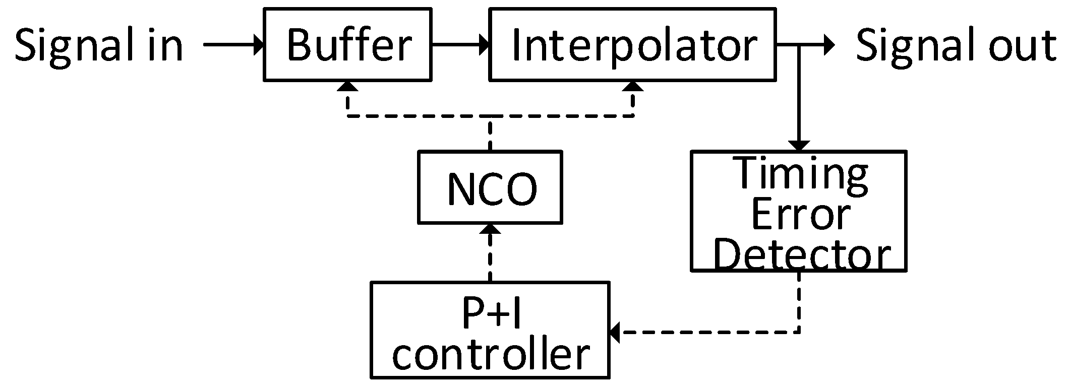
2. Clock Recovery in Coherent Optical Receivers

In communication systems, the synchronization between the sample rate, generated at the receiver clock, and the symbol rate, generated at the transmitter clock, is necessary for a correct extraction of the transmitted information [2]. The main objective of the symbol synchronization is then to determine, with the best precision as possible, the optimal decision instant where the signal has the maximum energy and signal-to-noise ratio.

Some synchronization solutions in literature use data-aided algorithms [23], which implies the transmission of a clock signal or a pre-determined symbol training sequence. However, such solutions require either higher power, to transmit an off-band clock tone, or higher transmission rates, to introduce an overhead, thus penalizing the transmission. On the other hand, non-data-aided algorithms [24,25] are capable of extracting the intrinsic timing information from the received signal, therefore, the success of such algorithms rely directly on the quantity and quality of the clock information available at the received signal. Factors such as bandwidth limitation, intersymbol interference or low signal-to-noise ratio tend to impair the performance of these methods.

Feedback Timing Synchronization Method

In the 1980’s, Gardner proposed a feedback algorithm that needed only two samples per symbol for timing estimation [24], resulting in low computational complexity. Figure 1 shows the implementation of the method.

This algorithm is based on the principle that PSK signals ideally have constant modulus. The signal power is maximal when the signal is sampled at the optimum decision instant, and it loses energy in the transitions between its constellation points. To illustrate it, Figure 2a shows a quadriphase shift keying (QPSK) constellation sampled at the optimum decision instants in red, and the transitions between symbols, in black. Figure 2b shows the eye diagram of the in-phase component, and Figure 2c shows the eye diagram of the power of the QPSK signal. The reader can note that while in the transitions, the signal power is lower on average, compared to the optimum decision instant.

Therefore, the algorithm tries to maximize the power of the received signal at the sampling instant by adjusting its timing. To achieve it, the timing error detector block in Figure 1 computes the Gardner timing error function, $e_{Gardner}$, given by the inflection point by the derivative of the power of the interpolator output, $b\left[n\right]$. Then,

$$\begin{array}{cc}\hfill e_{Gardner}\left[n\right]& =P_b^{\prime }\left[n\right]={\left(\overline{b}\left[n\right]b\left[n\right]\right)}^{\prime }={\overline{b}}^{\prime }\left[n\right]b\left[n\right]+\overline{b}\left[n\right]b^{\prime }\left[n\right]\hfill \\ & =\left(b_i^{\prime }\left[n\right]-j{b}_q^{\prime }\left[n\right]\right)\left(b_i\left[n\right]+j{b}_q\left[n\right]\right)+\left(b_i\left[n\right]-j{b}_q\left[n\right]\right)\left(b_i^{\prime }\left[n\right]+j{b}_q^{\prime }\left[n\right]\right)\hfill \\ & =2b_i\left[n\right]b_i^{\prime }\left[n\right]+2b_q\left[n\right]b_q^{\prime }\left[n\right],\hfill \end{array}$$

(1)

where n is the discrete index at 2 samples per symbol period, $P_b\left[n\right]$ is the power of interpolator output, $b_i\left[n\right]$ and $b_q\left[n\right]$ are, respectively, the real and imaginary parts of $b\left[n\right]$, the symbol ${}^{\prime }$ indicates the first derivative, and the overbar indicates the complex conjugate. Numerically approximating the signal derivative by

$$b^{\prime }\left[n\right]=\frac{1}{2}\left(b\left[n+1\right]-b\left[n-1\right]\right),$$

(2)

then, adjusting to make the signal causal and averaging through N symbols, the timing error function in average, ${\widehat{e}}_{Gardner}$, is defined by

$$\begin{array}{cc}\hfill {\widehat{e}}_{Gardner}& =\frac{1}{N}\sum _{n=0}^{N-1}\left\{b_i[2n-1]\left(b_i\left[2n\right]-b_i[2n-2]\right)+b_q[2n-1]\left(b_q\left[2n\right]-b_q[2n-2]\right)\right\}\hfill \\ & =\frac{1}{N}\Re \left\{\sum _{n=0}^{N-1}\left[b^{*}[2n-1]\left(b\left[2n\right]-b[2n-2]\right)\right]\right\}.\hfill \end{array}$$

(3)

where ℜ indicates the real part. Figure 2d shows all the possible values $e_{Gardner}\left[n\right]$ can assume, in black, and ${\widehat{e}}_{Gardner}$, in red. This last curve is known in the literature as the S-curve and can be used to indicate if the signal is late or in advance compared to the optimum decision instant.

The timing error function is then passed through a proportional-plus-integral controller (P + I) that filters and controls the clock frequency and phase of a numeric controlled oscillator (NCO) that will therefore drive the timing of the signal interpolators, locking when the timing error function is zero (in the middle of the S-curve).

Using Fourier transform properties, one can show that the Gardner’s timing error function, can be computed in frequency domain by [26]

$${\widehat{e}}_{Gardner}=\frac{2}{K}\sum _{k=1}^{K/2}\left\{sin\left(\frac{2\pi k}{K}\right)\Im \left(B\left[k\right]B[k+K/2]\right)\right\},$$

(4)

where ℑ indicates imaginary part, $B\left[k\right]$ is the discrete Fourier transform of $b\left[n\right]$, and K is the discrete Fourier transform length. This equation is similar to the one presented by Godard [25],

$${\widehat{e}}_{Godard}=\frac{2}{K}\sum _{k=1}^{K/2}\left\{\Im \left(B\right[k\left]B\right[k+K/2\left]\right)\right\},$$

(5)

and has been proven to yield similar results compared to the Gardner method [26].

The performance of the clock recovery algorithm can be therefore described by the amplitude of the S-curve. The clock tone amplitude (CTA) can be extracted by computing the absolute value instead of the imaginary part in ${\widehat{e}}_{Godard}$ [7],

$$CTA=\left|\sum _{k=1}^{K/2}B\left(k\right)B^{*}\left(k+K/2\right)\right|.$$

(6)

3. Matrix Propagation Model for Optical Fibers

3.1. Single-Mode Fibers without Coupling between Polarizations

Neglecting nonlinearities and noise, the transmission through an optical fiber can be described by

$${\mathbf{E}}_{out}(\Omega )=\mathbf{M}(\Omega ){\mathbf{E}}_{in}(\Omega ),$$

(7)

where $\mathbf{M}(\Omega )$ is a $2\times 2$ matrix describing the transfer characteristics of the optical fiber supporting 2 polarizations, and ${\mathbf{E}}_{in}(\Omega )$ and ${\mathbf{E}}_{out}(\Omega )$ are frequency-domain 2-dimensional input and output electrical field vectors.

Due to fabrication processes, single-mode fibers present birefringence, i.e., orthogonal polarization states will travel through the fiber at different speeds. If there is no coupling between polarization modes, then the fiber transfer characteristic can be described by

$$\mathbf{M}(\Omega )=\mathbf{V}\mathsf{\Lambda }(\Omega ){\mathbf{U}}^{†},$$

(8)

where $\mathbf{V}$ and $\mathbf{U}$ are random unitary rotation matrices describing coordinate base changes necessary due to the unknown spatial direction of the birefringence, and † indicates the conjugate transpose of the matrix. $\mathbf{V}$ and $\mathbf{U}$ are defined by

$$\mathbf{V},\mathbf{U}\stackrel{\mathrm{def}}{=}\left[\begin{array}{cc}cos\left(\theta \right)& sin\left(\theta \right)e^{j\varphi }\\ -sin\left(\theta \right)& cos\left(\theta \right)e^{j\varphi }\end{array}\right],$$

(9)

where $\theta$ and $\varphi$ are the azimuth and ellipticity angles of the unitary rotation matrix. $\mathsf{\Lambda }(\Omega )$ is a diagonal matrix describing the linear propagation in each of the polarization modes. Including polarization dependent loss (PDL), differential group delay (DGD), and chromatic dispersion (CD). $\mathsf{\Lambda }(\Omega )$ can be expressed by

$$\mathsf{\Lambda }(\Omega )=\mathrm{diag}\left[a_1(\Omega ),a_2(\Omega )\right],$$

(10)

$$a_1(\Omega )=exp\left\{{\displaystyle \frac{g_1}{2}}-j{\displaystyle \frac{\tau L}{2}}\Omega -jD{\displaystyle \frac{{\lambda }^{2}L}{4\pi c}}{\Omega }^2+jS{\displaystyle \frac{{\lambda }^{4}L}{24{\pi }^2{c}^2}}{\Omega }^3\right\},$$

(11)

$$a_2(\Omega )=exp\left\{{\displaystyle \frac{g_2}{2}}+j{\displaystyle \frac{\tau L}{2}}\Omega -jD{\displaystyle \frac{{\lambda }^{2}L}{4\pi c}}{\Omega }^2+jS{\displaystyle \frac{{\lambda }^{4}L}{24{\pi }^2{c}^2}}{\Omega }^3\right\},$$

(12)

where $\mathbf{g}=\left[g_1,g_2\right]$ is the PDL vector, $\tau$ is the DGD, related to polarization mode dispersion (PMD), D is the CD parameter, S is the fiber dispersion slope, related to third-order CD, and L is the length of the fiber.

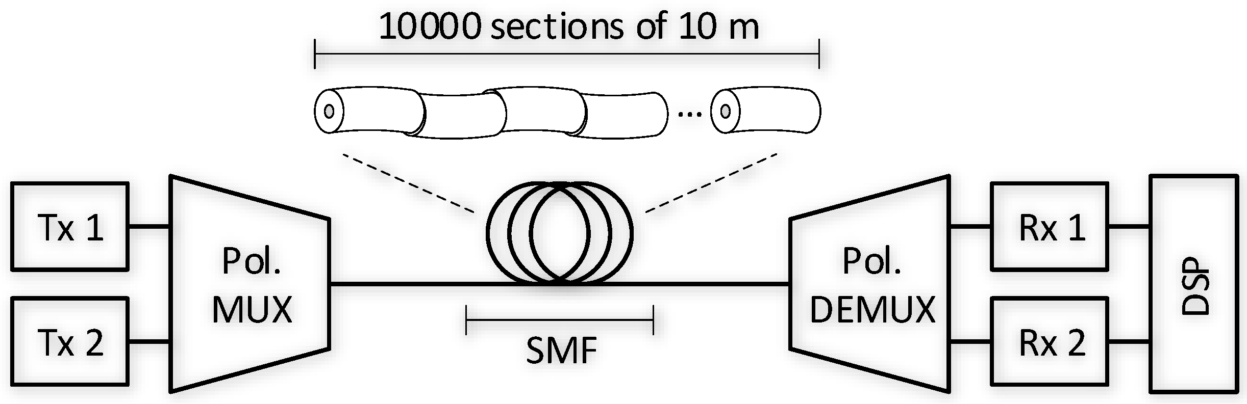
3.2. Single-Mode Fibers with Strong Coupling between Polarizations

Due to bends and stretches, the birefringence will vary throughout the fiber, making it impractical to design long optical fibers with no coupling between polarizations. Consequently, the differential group delay can be a limiting factor for optical communications. To overcome this issue, SMFs are fabricated with intentional birefringence rotations in order to average out the group delay [27]. Therefore, a common numerical approximation for the fiber model is to consider the optical fiber as the concatenation of shorter sections of fiber (Figure 3). Each of these sections is a piece of fiber that has length slightly longer than the length over which the complex polarization fields remain correlated [28] and has no coupling between polarizations, but both random rotations at the input and at the output occur. Moreover, the DGD is kept constant in each fiber section.

Then, considering $K_{sec}$ sections of a fiber with each of these sections having length $L_{sec}$, and neglecting noise and nonlinearities, the signal at each fiber section output is related to the its input signal by

$${\mathbf{E}}_{out}^{\left(k\right)}(\Omega )={\mathbf{M}}^{\left(k\right)}(\Omega ){\mathbf{E}}_{in}^{\left(k\right)}(\Omega ),$$

(13)

where k is the section index. The full fiber transfer characteristic is, then,

$$\mathbf{M}(\Omega )=\prod _{k=1}^{K_{sec}}{\mathbf{V}}^{\left(k\right)}{\mathsf{\Lambda }}^{\left(k\right)}(\Omega ){\mathbf{U}}^{\left(k\right)†}.$$

(14)

3.3. Multi-Mode and Multi-Core Fibers

Generalizing the model for both single- and multi-mode fibers, the transfer function characteristic, $\mathbf{M}(\Omega )$, can be extended and take the form of a Z × Z matrix, where Z is the number of all possible spatial degrees of freedom, and ${\mathbf{E}}_{in}(\Omega )$ and ${\mathbf{E}}_{out}(\Omega )$ are frequency-domain Z-dimensional input and output electrical field vectors. The term “degrees of freedom” includes both the two polarizations in a SMF ($Z=2$) and all possible spatial degrees of freedom in a FMF ($Z=2P>2$, where P is the number of modes). The matrix ${\mathsf{\Lambda }}^{\left(k\right)}(\Omega )$ can be expressed as

$${\mathsf{\Lambda }}^{\left(k\right)}(\Omega )=\mathrm{diag}\left[a_1(\Omega ),a_2(\Omega ),\cdots ,a_Z(\Omega )\right],$$

(15)

$$a_d(\Omega )=exp\left\{{\displaystyle \frac{g_z^{\left(k\right)}}{2}}-j{\tau }_z^{\left(k\right)}\Omega -j{\displaystyle \frac{D_z{\lambda }^2{L}_{sec}}{4\pi c}}{\Omega }^2+j{\displaystyle \frac{S_z{\lambda }^4{L}_{sec}}{24{\pi }^2{c}^2}}{\Omega }^3\right\},z\in \left[1,2,\cdots ,Z\right],$$

(16)

where ${\mathbf{g}}^{\left(k\right)}=\left[\begin{array}{c}{g}_1^{\left(k\right)},g_2^{\left(k\right)},\dots ,g_Z^{\left(k\right)}\end{array}\right]$ is the uncoupled mode-dependent loss (MDL) vector, ${\tau }^{\left(k\right)}=\left[\begin{array}{c}{{\tau }_1}^{\left(k\right)},{{\tau }_2}^{\left(k\right)},\dots ,{{\tau }_Z}^{\left(k\right)}\end{array}\right]$ is the group delay vector, related to the mode delay (MD), $\mathbf{D}=\left[\begin{array}{c}{D}_1,D_2,\dots ,D_Z\end{array}\right]$ is the CD vector, and $\mathbf{S}=\left[\begin{array}{c}{S}_1,S_2,\dots ,S_Z\end{array}\right]$ is the fiber dispersion slope vector.

${\mathbf{V}}^{\left(k\right)}$ and ${\mathbf{U}}^{\left(k\right)}$ are random Z × Z unitary matrices generated by random Givens’ rotation matrices [29]:

$${\mathbf{V}}^{\left(k\right)},{\mathbf{U}}^{\left(k\right)}\stackrel{\mathrm{def}}{=}\prod _{i=1}^{Z-1}\prod _{k=i+1}^Z\mathbf{G}\left(i,k,{\theta }_{i,k},{\varphi }_{i,k}\right),$$

(17)

where each element $g_{m,n}$ of $\mathbf{G}$ is given by:

$$g_{m,n}=\left\{\begin{array}{cc}cos\left({\theta }_{i,k}\right),\hfill & \mathrm{if}m=n=i\hfill \\ cos\left({\theta }_{i,k}\right)e^{j{\varphi }_{i,k}},\hfill & \mathrm{if}m=n=k\hfill \\ sin\left({\theta }_{i,k}\right)e^{j{\varphi }_{i,k}},\hfill & \mathrm{if}m=i\mathrm{and}n=k\hfill \\ -sin\left({\theta }_{i,k}\right),\hfill & \mathrm{if}m=k\mathrm{and}n=i\hfill \\ 1,\hfill & \mathrm{if}m=n\ne i\mathrm{or}m=n\ne k\hfill \\ 0,\hfill & \mathrm{otherwise}.\hfill \end{array}\right.$$

(18)

In the single-mode case, $Z=2$, the rotation matrix from Equation (17) assumes the same form of Equation (9). The Givens’ rotation matrices are basically rotations relative to an axis, therefore to generate the Z × Z unitary matrices, we generate random rotations relative to all possible axes.

3.4. Time Skew between Polarizations and Modes

Another parameter that can affect the clock recovery performance is the time skew between signal components [22]. So, apart from the DGD, the signal components can be time mismatched due to propagation differences in the electrical cables both at the transmitter and the receiver. We can model the time skew between signal components, $\mathbf{W}(\Omega )$, by:

$$\mathbf{W}(\Omega )=\mathrm{diag}\left[exp\{-j\Omega {\tau }_1\},exp\{-j\Omega {\tau }_2\},\cdots ,exp\{-j\Omega {\tau }_Z\}\right].$$

(19)

Therefore, regarding the time skews, the received signal is related to the input signal by,

$${\mathbf{E}}_{out}(\Omega )={\mathbf{W}}_{Rx}(\Omega )\mathbf{M}(\Omega ){\mathbf{W}}_{Tx}(\Omega ){\mathbf{E}}_{in}(\Omega ).$$

(20)

In the next sections, we will analyze the clock recovery performance evaluating the clock tone amplitude for the QPSK modulation format. Higher-order QAM modulation formats are expected to have similar performance as the spectrum shape of these formats are invariant to the modulation order [30].

4. Clock Recovery Performance in Single-Mode Fibers

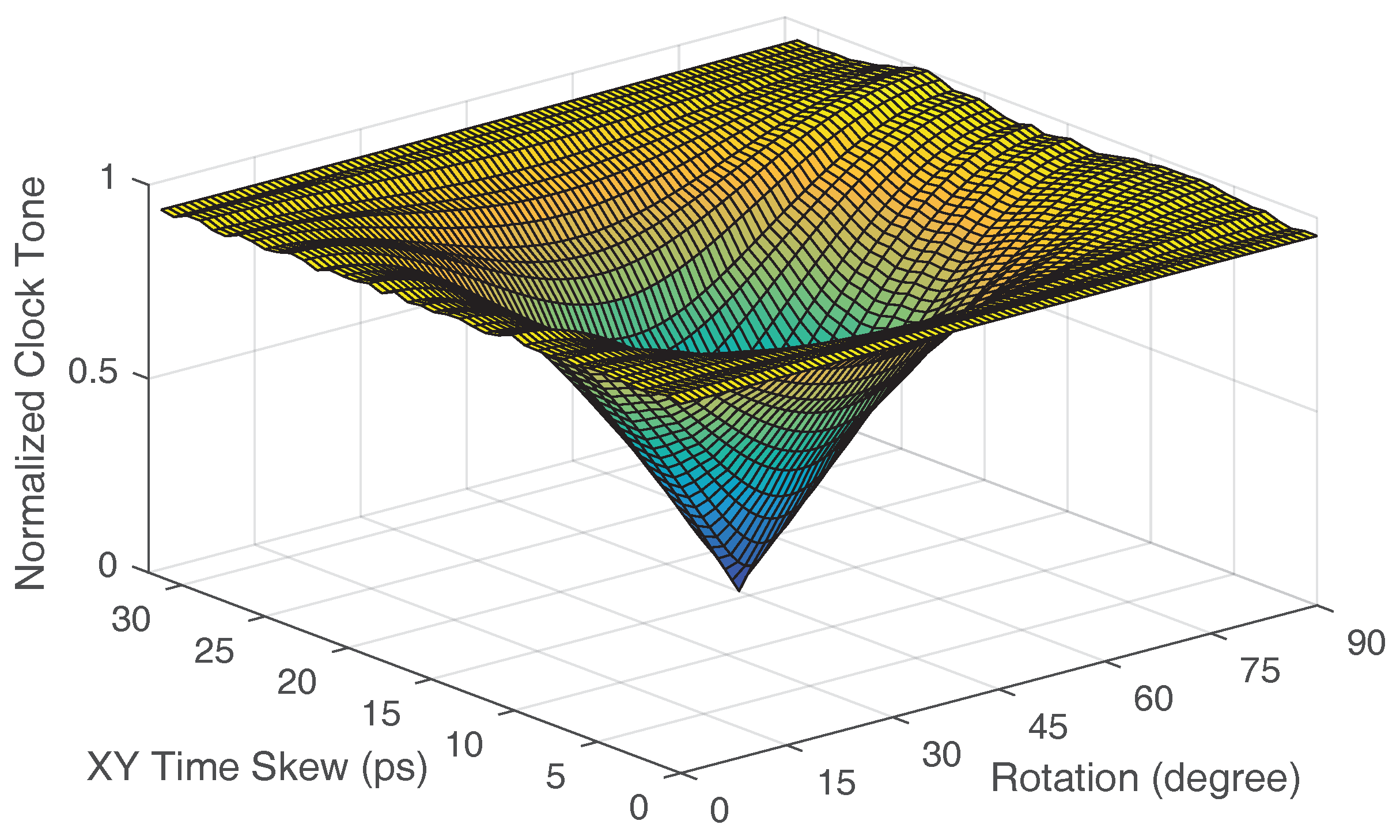
4.1. Time Skew between Polarizations

First, to evaluate the impact of the time skew between polarizations we considered a back-to-back system with the time skew both in the transmitter and the receiver. We also considered a polarization azimuth rotation between transmitter and receiver. For simplicity, the ellipticity rotations were not considered. The transfer function of this simulation was then,

$${\mathbf{E}}_{out}(\Omega )=\left[\begin{array}{cc}{e}^{-j\Omega {\tau }_{Rx}/2}& 0\\ 0& e^{j\Omega {\tau }_{Rx}/2}\end{array}\right]\left[\begin{array}{cc}cos\left(\theta \right)& sin\left(\theta \right)\\ -sin\left(\theta \right)& cos\left(\theta \right)\end{array}\right]\left[\begin{array}{cc}{e}^{-j\Omega {\tau }_{Tx}/2}& 0\\ 0& e^{j\Omega {\tau }_{Tx}/2}\end{array}\right]{\mathbf{E}}_{in}(\Omega ),$$

(21)

where ${\tau }_{Tx}$ was the time skew between polarizations at the transmitter, ${\tau }_{Rx}$ was the time skew between polarizations at the receiver, and $\theta$ the rotation angle. The received signal in polarization X is then,

$${\mathbf{E}}_{out,X}=e^{-j\Omega {\tau }_{Rx}/2}\left(e^{-j\Omega {\tau }_{Tx}/2}cos\left(\theta \right){\mathbf{E}}_{in,X}+e^{j\Omega {\tau }_{Tx}/2}sin\left(\theta \right){\mathbf{E}}_{in,Y}\right).$$

(22)

Therefore, the received signal is a combination of the transmitted signal in both polarizations with opposite timings due to the transmitter inter-polarization time skew. On the other hand, the receiver time skew only delays the transmitted signal components with the same timing. Thus, it is expected that the transmitter inter-polarization time skew will affect the clock tone amplitude depending on the polarization rotation during transmission, while the receiver time skew will not affect it. To show this behavior, we then considered an NRZ-QPSK at 32 GBd as signal input and swept the rotation angle from 0 to 90 degrees and the transmitter time skew from 0 to 31.125 ps, equivalent to the interval from 0 to 1 symbol period. The parameters used in this simulation are summarized in

Table 1. Parameters for B2B evaluation of CTA due to transmitter time skew.

Parameter	Value
Modulation format	NRZ-QPSK
Symbol rate	32 GBd
Rotation angle interval	$[0,90°]$
Rotation angle step size	$1°$
Transmitter time skew interval	$[0,31.125]$ ps
Transmitter time skew step size	$778.125$ fs
Receiver time skew	0

. The receiver time skew was set to zero. The CTA was computed and it is shown in Figure 4.

As we can see, the CTA goes to zero when the rotation angle is 45 degrees and the inter-polarization time skew in the transmitter is around half symbol period. This means that estimation and compensation of inter-polarization time skews at the transmitter side is crucial.

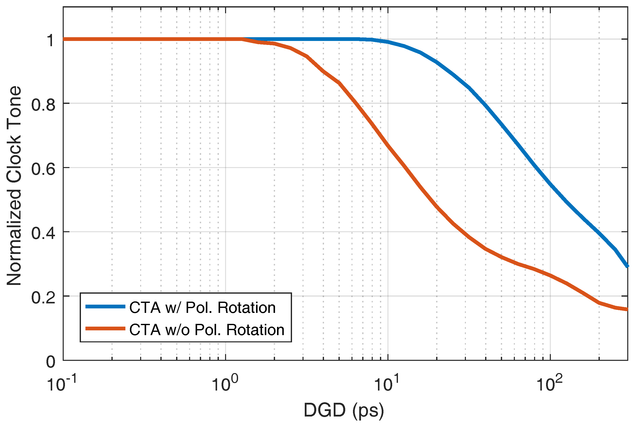
4.2. Polarization Mode Dispersion

In order to analyze the clock recovery performance in single-mode fibers, we used the configuration as shown in Figure 5. We consider 32 GBd non-return-to-zero (NRZ)-QPSK modulated signals multiplexed in $Z=2$ degrees of freedom (two polarizations). The transmission link was simulated numerically and consisted of a single-mode fiber with strong coupling between polarizations divided in 10,000 sections of fiber with 10 m each [27], resulting in a 100 km fiber link.

To evaluate the behavior of timing recovery with different values of DGD, we considered random Givens rotation matrices and swept the group delay of each fiber segment, i.e., each segment had a random rotation with an angle uniformly distributed in the interval $\theta \sim [0,2\pi )$. We swept the uncoupled DGD from $0.005$ to 500 ps/km, i.e., the propagation delay difference between polarizations in each fiber section. Then, we measured the resulting DGD by the maximum difference of the two eigenvalues of the matrix, $\mathbf{H}(\Omega )$, defined by [11]

$$\mathbf{H}(\Omega )=j\frac{\partial \mathbf{M}(\Omega )}{\partial \Omega }{\mathbf{M}}^{*}(\Omega ),$$

(23)

with the differentiation being computed numerically. This resulting DGD is the DGD after all rotations between sections and discrete delays. The parameters used in this simulation are summarized in

Table 2. Parameters for evaluation of CTA due to PMD in single-mode fiber transmission.

Parameter	Value
Modulation format	NRZ-QPSK
Symbol rate	32 GBd
Number of fiber sections	10,000
Fiber length per section	10 m
Total fiber length	100 km
Rotation angle per section	uniform distribution $\sim [0,360°)$
Uncoupled DGD interval	$[0.005,500]$ ps/km
Uncoupled DGD step size	$25.89\%$ greater every iteration
Transmitter time skew	0
Receiver time skew	0

.

We considered both the CTA extracted directly from the received signal at polarization X, ${\mathbf{E}}_{out,X}$, and also the CTA extracted by a combination of the polarizations X and Y, ${\mathbf{E}}_{out,XY}$, given by

$${\mathbf{E}}_{out,XY}={\mathbf{E}}_{out,X}cos\left(\varphi \right)+{\mathbf{E}}_{out,Y}sin\left(\varphi \right),$$

(24)

where $\varphi$ is the angle that is tracked maximizing the CTA value [7]. The results are shown in Figure 6.

We can see by Figure 6 that using the polarization rotation method [7], the CTA remain at the maximum level until a resulting DGD of 10 ps. Since a typical modern single-mode fiber has PMD parameter around 0.1 $\mathrm{ps}/\sqrt{\mathrm{km}}$, the CTA would only be degraded after 10,000 km, needing at least ten times this transmission distance to drop the CTA to half of its maximum value. Therefore, for all practical applications the vanishing of clock tone is not a problem for polarization multiplexed transmission through single-mode fibers.

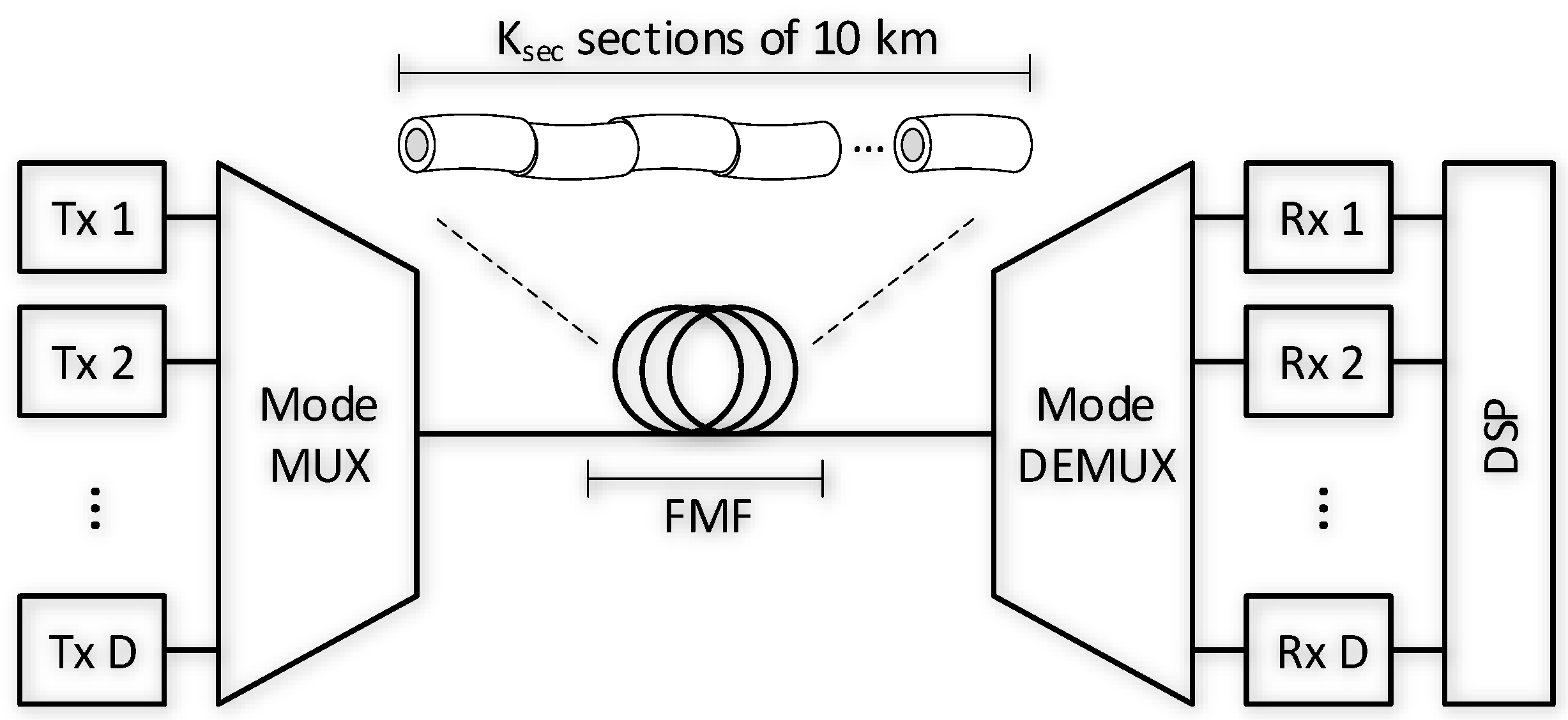
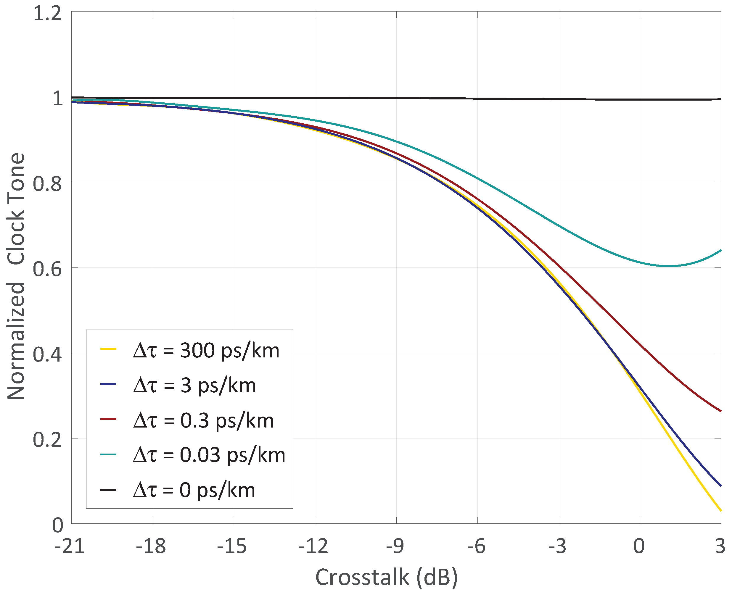
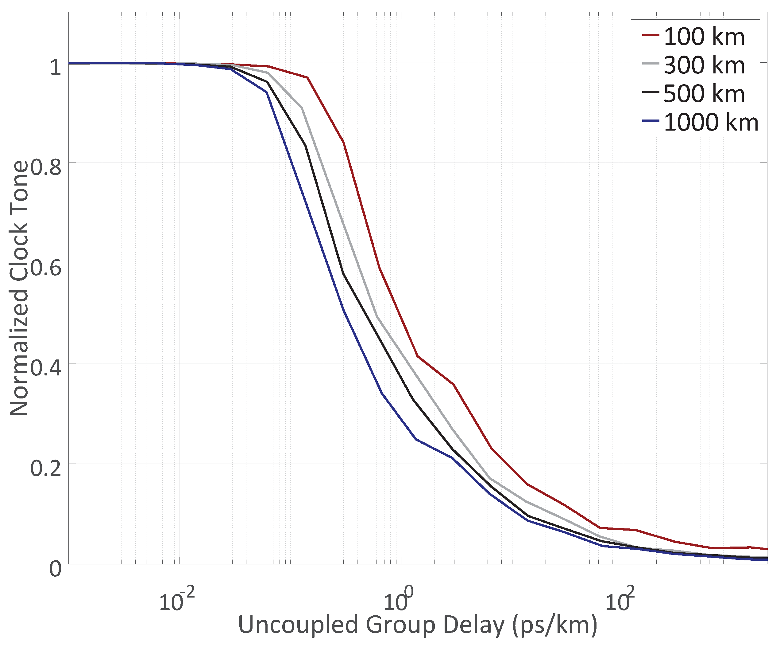
5. Clock Recovery Performance in Multi-Mode Fibers

In order to analyze clock recovery performance in multi-mode systems we used the general configuration as shown in Figure 7. We considered 32 GBd NRZ-QPSK modulated signals spatially multiplexed in $Z=6$ degrees of freedom. The transmission link was simulated numerically and consisted of a 3-mode FMF divided in sections of 10 km, with two degrees of freedom per mode. In the receiver DSP, the clock extraction and resampling was performed before dynamic MIMO equalization to enable the equalizer to keep up with slow timing drifts in steady state operation. The clock extraction was performed per mode, so we had one value of clock tone magnitude for each of the modes.

To evaluate the behavior of timing synchronization in different coupling regimes, we swept the rotation distribution of the unitary matrices ${\mathbf{V}}^{\left(k\right)}$ and ${\mathbf{U}}^{\left(k\right)}$ in Equation (17), measuring the crosstalk into the fundamental mode group due to high order mode groups. The parameters used in this simulation are summarized in

Table 3. Parameters for evaluation of CTA due to PMD in single-mode fiber transmission.

Parameter	Value
Modulation format	NRZ-QPSK
Symbol rate	32 GBd
Number of degrees of freedom	6
Fiber length per section	10 km
Total fiber length (Figure 8)	1000 km
Total fiber length (Figure 9)	100, 300, 500 and 1000 km
Uncoupled group delay (Figure 8)	0, 0.03, 0.3, 3 and 300 ps/km
Uncoupled group delay interval (Figure 9)	$[0.001,1000]$ ps/km
Rotation angle per section	zero-mean normal distribution
Rotation angle variance interval	$[0,2000°]$
Transmitter time skew	0
Receiver time skew	0

. For simplicity we did not distinguish between inter- and intra-mode group coupling. We are not considering any losses, non-linearities and chromatic dispersion.

We show in Figure 8 the results for a 1000 km transmission of 3-mode FMF. This fiber has two mode groups, two degrees of freedom (one mode) on fundamental group and four degrees of freedom (two modes) in the second group. Here, the crosstalk is the ratio of the contribution of the second mode group into the fundamental mode. We define a strong coupling regime when the crosstalk is approximately 3 dB, the weak coupling regime when the crosstalk is lower than −18 dB and refer to intermediate coupling regime for the region in-between. The results shown are the average of 10 random simulations for each crosstalk value in a system with no losses or chromatic dispersion.

Here, we parametrize the curves using the uncoupled group delay, $\Delta \tau$, which is the time difference between the fastest and the slowest modes’ group velocities. As expected for zero group delay, the clock tone remained unchanged at the maximum value irrespective of the crosstalk. However, increasing the uncoupled group delay, we saw a dramatic drop in the clock tone quality. In the strong coupling case, an uncoupled group delay of less than 0.03 ps/km was required in order to still have a detectable clock tone higher than 50% of the maximum value.

We also evaluated the behavior of clock tone quality for strong coupling regime as a function of uncoupled group delay for different transmission distances. Results are shown in Figure 9. The clock tone quality drops for smaller values of uncoupled group delay as the transmission distance increases, so for long-haul MDM transmission the delay spread requirements are even tighter.

6. Conclusions

We showed through simulations that the inter-polarization time skew, polarization rotation, and PMD can be compensated in optical systems employing single-mode fibers and, therefore, will not affect the performance of clock synchronization. Particularly, it would need more than 10,000 km of a modern fiber with DGD of 0.1 ps/$\sqrt{\mathrm{km}}$ in order to be able to see some impact of DGD on the clock recovery performance. However, in multi-mode systems the mode coupling and delay spread could have a impact much worse in the performance of timing synchronization. It was demonstrated although strong coupling reduces the coupled group delay spread [11] and nonlinearities [19], the clock tone will completely vanish even for very low group delays, making timing synchronization unfeasible. In order to have a detectable clock tone higher than 50% of the maximum value, the multi-mode optical fiber would need to have an impractical uncoupled group delay of less than $0.03$ ps/km. Also, we showed that increasing the transmission distance will reduce the group delay tolerance of MDM systems even more under strong coupling regime. Possible solutions could be use of pilot tones for timing synchronization or operation in weak coupling regime with sparsity managed MIMO equalizers [17,18]. Other transmission impairments such as the equalization enhanced phase noise [31] and fiber nonlinearities [32] could possibly impact the clock recovery performance and are planned to be analyzed in future works.

References

1. Agrell, E.; Karlsson, M.; Chraplyvy, A.R.; Richardson, D.J.; Krummrich, P.M.; Winzer, P.; Roberts, K.; Fischer, J.K.; Savory, S.J.; Eggleton, B.J.; et al. Roadmap of optical communications. J. Opt. 2016, 18, 063002. [Google Scholar] [CrossRef] [Green Version]
2. Savory, S.J. Digital Coherent Optical Receivers: Algorithms and Subsystems. IEEE J. Sel. Top. Quantum Electron. 2010, 16, 1164–1179. [Google Scholar] [CrossRef]
3. Zibar, D.; Bianciotto, A.; Wang, Z.; Napoli, A.; Spinnler, B. Analysis and Dimensioning of Fully Digital Clock Recovery for 112 Gb/s Coherent Polmux QPSK Systems. In Proceedings of the 2009 35th European Conference on Optical Communication (ECOC), Vienna, Austria, 20–24 September 2009. [Google Scholar]
4. Sun, H.; Wu, K.T. A novel dispersion and PMD tolerant clock phase detector for coherent transmission systems. In Proceedings of the Optical Fiber Communication Conference (OFC), Los Angeles, CA, USA, 6–10 March 2011. [Google Scholar]
5. Zibar, D.; de Oliviera, J.C.R.; Ribeiro, V.B.; Paradisi, A.; Diniz, J.C.; Larsen, K.J.; Monroy, I.T. Experimental Investigation of Digital Compensation of DGD for 112 Gb/s PDM-QPSK Clock Recovery. In Proceedings of the European Conference on Optical Communication (ECOC), Geneva, Switzerland, 18–22 Septmner 2011. [Google Scholar]
6. Zibar, D.; de Olivera, J.C.R.F.; Ribeiro, V.B.; Paradisi, A.; Diniz, J.C.; Larsen, K.J.; Monroy, I.T. Experimental investigation and digital compensation of DGD for 112 Gb/s PDM-QPSK clock recovery. Opt. Express 2011, 19, B429–B439. [Google Scholar] [CrossRef] [PubMed]
7. Stojanović, N.; Xie, C.; Zhao, Y.; Mao, B.; Guerrero Gonzalez, N. A Circuit enabling Clock Extraction in Coherent Receivers. In Proceedings of the European Conference on Optical Communication (ECOC), Amsterdam, Netherlands, 16–20 September 2012. [Google Scholar]
8. Birk, M.; Gerard, P.; Curto, R.; Nelson, L.E.; Zhou, X.; Magill, P.; Schmidt, T.J.; Malouin, C.; Zhang, B.; Ibragimov, E.; et al. Coherent 100 Gb/s PM-QPSK field trial. IEEE Commun. Mag. 2010, 48, 52–60. [Google Scholar] [CrossRef]
9. Winzer, P. Spatial Multiplexing: The Next Frontier in Network Capacity Scaling. In Proceedings of the European Conference on Optical Communication (ECOC), London, UK, 22–26 September 2013. [Google Scholar]
10. Winzer, P.J.; Neilson, D.T. From Scaling Disparities to Integrated Parallelism: A Decathlon for a Decade. J. Lightwave Technol. 2017, 35, 1099–1115. [Google Scholar] [CrossRef]
11. Arik, S.O.; Ho, K.P.; Kahn, J.M. Group Delay Management and Multiinput Multioutput Signal Processing in Mode-Division Multiplexing Systems. J. Lightwave Technol. 2016, 34, 2867–2880. [Google Scholar] [CrossRef]
12. Randel, S.; Ryf, R.; Sierra, A.; Winzer, P.J.; Gnauck, A.H.; Bolle, C.A.; Essiambre, R.J.; Peckham, D.W.; McCurdy, A.; Lingle, R. 6×56-Gb/s mode-division multiplexed transmission over 33-km few-mode fiber enabled by 6 × 6 MIMO equalization. Opt. Express 2011, 19, 16697–16707. [Google Scholar] [CrossRef] [PubMed]
13. Randel, S.; Sierra, A.; Mumtaz, S.; Tulino, A.; Ryf, R.; Winzer, P.; Schmidt, C.; Essiambre, R. Adaptive MIMO signal processing for mode-division multiplexing. In Proceedings of the Optical Fiber Communication Conference and Exposition (OFC), Los Angeles, CA, USA, 4–8 March 2012. [Google Scholar]
14. Randel, S.; Winzer, P. DSP for mode division multiplexing. In Proceedings of the OptoElectronics and Communications Conference/Photonics in Switching (OECC/PS), Kyoto, Japan, 30 June–4 July 2013. [Google Scholar]
15. Arik, S.O.; Askarov, D.; Kahn, J.M. Adaptive Frequency-Domain Equalization in Mode-Division Multiplexing Systems. J. Lightwave Technol. 2014, 32, 1841–1852. [Google Scholar] [CrossRef]
16. Asif, R.; Ye, F.; Morioka, T. Equalizer complexity for 6-LP mode 112 Gbit/s m-ary DP-QAM space division multiplexed transmission in strongly coupled Few-Mode-Fibers. In Proceedings of the 2015 European Conference on Networks and Communications (EuCNC), Paris, France, 29 June–2 July 2015. [Google Scholar]
17. Shi, K.; Thomsen, B.C. Sparse Adaptive Frequency Domain Equalizers for Mode-Group Division Multiplexing. J. Lightwave Technol. 2015, 33, 311–317. [Google Scholar] [CrossRef] [Green Version]
18. Lee, D.; Shibahara, K.; Kobayashi, T.; Mizuno, T.; Takara, H.; Sano, A.; Kawakami, H.; Nakagawa, T.; Miyamoto, Y. A Sparsity Managed Adaptive MIMO Equalization for Few-Mode Fiber Transmission with Various Differential Mode Delays. J. Lightwave Technol. 2016, 34, 1754–1761. [Google Scholar] [CrossRef]
19. Ferreira, F.; Suibhne, N.M.; Sánchez, C.; Sygletos, S.; Ellis, A.D. Advantages of Strong Mode Coupling for Suppression of Nonlinear Distortion in Few-Mode Fibers. In Proceedings of the Optical Fiber Communications Conference and Exhibition (OFC), Anaheim, CA, USA, 20–22 March 2016. [Google Scholar]
20. Antonelli, C.; Mecozzi, A.; Shtaif, M. Scaling of inter-channel nonlinear interference noise and capacity with the number of strongly coupled modes in SDM systems. In Proceedings of the Optical Fiber Communications Conference and Exhibition (OFC), Anaheim, CA, USA, 20–22 March 2016; pp. 1–3. [Google Scholar]
21. Diniz, J.C.M.; Piels, M.; Zibar, D. Performance Evaluation of Clock Recovery for Coherent Mode Division Multiplexed Systems. In Proceedings of the Optical Fiber Communication Conference, Los Angeles, CA, USA, 19–23 March 2017. [Google Scholar]
22. Diniz, J.C.M.; Da Ros, F.; da Silva, E.P.; Jones, R.T.; Zibar, D. Optimization of DP-M-QAM Transmitter Using Cooperative Coevolutionary Genetic Algorithm. J. Lightwave Technol. 2018, 36, 2450–2462. [Google Scholar] [CrossRef] [Green Version]
23. Mueller, K.; Muller, M. Timing Recovery in Digital Synchronous Data Receivers. IEEE Trans. Commun. 1976, 24, 516–531. [Google Scholar] [CrossRef]
24. Gardner, F. A BPSK/QPSK Timing-Error Detector for Sampled Receivers. IEEE Trans. Commun. 1986, 34, 423–429. [Google Scholar] [CrossRef]
25. Godard, D. Passband Timing Recovery in an All-Digital Modem Receiver. IEEE Trans. Commun. 1978, 26, 517–523. [Google Scholar] [CrossRef]
26. Huang, L.; Wang, D.; Lau, A.P.T.; Lu, C.; He, S. Performance analysis of blind timing phase estimators for digital coherent receivers. Opt. Express 2014, 22, 6749–6763. [Google Scholar] [CrossRef] [PubMed]
27. Agrawal, G.P. Fiber-Optic Communication Systems; John Wiley & Sons, Inc.: Hoboken, NJ, USA, 2010. [Google Scholar]
28. Ho, K.P.; Kahn, J.M. Mode Coupling and its Impact on Spatially Multiplexed Systems. In Optical Fiber Telecommunications; Kaminow, I., Li, T., Willner, A., Eds.; Academic Press: Cambridge, MA, USA, 2013; Volume VIB, Chapter 11; pp. 491–568. [Google Scholar]
29. Givens, W. Computation of Plain Unitary Rotations Transforming a General Matrix to Triangular Form. J. Soc. Ind. Appl. Math. 1958, 6, 26–50. [Google Scholar] [CrossRef]
30. Ip, E.; Kahn, J.M. Power spectra of return-to-zero optical signals. J. Lightwave Technol. 2006, 24, 1610–1618. [Google Scholar] [CrossRef]
31. Colavolpe, G.; Foggi, T.; Forestieri, E.; Secondini, M. Impact of Phase Noise and Compensation Techniques in Coherent Optical Systems. J. Lightwave Technol. 2011, 29, 2790–2800. [Google Scholar] [CrossRef] [Green Version]
32. Czegledi, C.B.; Liga, G.; Lavery, D.; Karlsson, M.; Agrell, E.; Savory, S.J.; Bayvel, P. Digital backpropagation accounting for polarization-mode dispersion. Opt. Express 2017, 25, 1903. [Google Scholar] [CrossRef] [PubMed] [Green Version]
Figure 1. Timing recovery implementation.
Futureinternet 10 00059 g001
Figure 2. (a) QPSK constellation, in red, with its intersymbol transitions, in black; (b) In-phase component eye-diagram; (c) Power eye-diagram; (d) S-curve, in red, and all values e G a r d n e r can assume in a QPSK signal, in black.
Futureinternet 10 00059 g002
Figure 3. Strong-coupling optical fiber model as the concatenation of shorter fiber sections.
Futureinternet 10 00059 g003
Figure 4. Normalized clock tone amplitude as function of rotation angle and transmitter-side inter-polarization time skew.
Futureinternet 10 00059 g004
Figure 5. General set-up for numerical simulation model of polarization multiplexed systems.
Futureinternet 10 00059 g005
Figure 6. Normalized clock tone amplitude as function of resulting DGD for a single-mode fiber.
Futureinternet 10 00059 g006
Figure 7. General set-up for numerical simulation model of multi-mode multiplexed systems.
Futureinternet 10 00059 g007
Figure 8. Normalized clock tone amplitude as a function of crosstalk between mode groups in a 1000 km transmission of a 3-mode FMF for different values of uncoupled group delay.
Futureinternet 10 00059 g008
Figure 9. Normalized clock tone amplitude as a function of uncoupled group delay between mode groups in a 3-mode FMF for distinct transmission distances.
Futureinternet 10 00059 g009