Abstract
American chestnut (Castanea dentata Borkh.) was a dominant tree species in its native range in eastern North America until the accidentally introduced fungus Cryphonectria parasitica (Murr.) Barr, that causes chestnut blight, led to a collapse of the species. Different approaches (e.g., genetic engineering or conventional breeding) are being used to fight against chestnut blight and to reintroduce the species with resistant planting stock. Because of large climatic differences within the distribution area of American chestnut, successful reintroduction of the species requires knowledge and consideration of local adaptation to the prevailing environmental conditions. Previous studies revealed clear patterns of genetic diversity along the northeast-southwest axis of the Appalachian Mountains, but less is known about the distribution of potentially adaptive genetic variation within the distribution area of this species. In this study, we investigated neutral and potentially adaptive genetic variation in nine American chestnut populations collected from sites with different environmental conditions. In total, 272 individuals were genotyped with 24 microsatellite (i.e., simple sequence repeat (SSR)) markers (seven genomic SSRs and 17 EST-SSRs). An FST-outlier analysis revealed five outlier loci. The same loci, as well as five additional ones, were significantly associated with environmental variables of the population sites in an environmental association analysis. Four of these loci are of particular interest, since they were significant in both methods, and they were associated with environmental variation, but not with geographic variation. Hence, these loci might be involved in (temperature-related) adaptive processes in American chestnut. This work aims to help understanding the genetic basis of adaptation in C. dentata, and therefore the selection of suitable provenances for further breeding efforts.
1. Introduction
American chestnut (Castanea dentata Borkh.) has been a dominant tree species in its distribution range in eastern North America and one of the ecologically and economically most important species in that region [1,2,3]. The accidentally introduced fungus Cryphonectria parasitica (Murr.) Barr, that causes chestnut blight, dramatically reduced the number and vitality of chestnut trees, so that the species nowadays occurs mainly as a vegetative propagating (from stump sprouts) understory shrub [1,3,4]. Mainly three different approaches have been used to fight against chestnut blight [1]: inoculation of diseased trees with hypovirulent strains of C. parasitica, genetic engineering, and breeding of resistant trees. Treatment of cankers with hypoviruses is effective in intensively managed plantations or orchards and hypoviruses naturally occur in Michigan (USA), but biological control with hypovirulence has not been successful in forest populations in North America [5]. Genetic engineering of resistant trees has made substantial progress, but is currently limited by public acceptance and regulatory and legal restrictions. For instance, genetically modified trees to be grown in North America must be sterile or have some other means to control flowering [6], and hence, natural repopulation by sexual reproduction is impossible. Large efforts have also been made in conventional breeding to establish blight resistant chestnut trees. Specifically, backcross breeding was used to incorporate blight resistance from Chinese chestnut (Castanea mollissima Blume) into C. dentata, resulting in hybrid trees that show a lower disease incidence [7,8,9]. The development of new genomic resources [10,11,12,13,14] for different Castanea species will help to enhance breeding success for disease resistance.
Because of large climatic differences within the distribution area of American chestnut, a successful reintroduction of the species requires knowledge and consideration of local adaptation to the prevailing environmental conditions. For instance, there are indications that hybrid backcrossed chestnut trees are less cold tolerant than pure American chestnut trees [15]. Different studies investigated the distribution of genetic diversity based on different genetic markers in American chestnut populations in North America. Thus, the highest genetic diversity was detected in southwestern populations with a decrease along the Appalachian Mountains to the northeast [16,17]. Furthermore, a clinal variation of allele frequencies was observed along the Appalachian axis [16,17,18]. The observed distribution of genetic variation is most likely an effect of postglacial recolonization. Refugial areas of American chestnut were likely located far south along the Gulf Coast and the species re-migrated comparatively slowly to the north arriving in Connecticut (northeast USA) only about 2000 years ago [19,20]. Less is known, however, about the distribution of potentially adaptive genetic variation within the distribution area of American chestnut. Therefore, we investigated neutral and potentially adaptive genetic variation in nine American chestnut populations growing under different climatic conditions. The same populations were analyzed previously by Gailing and Nelson [16] with partly overlapping markers (17 EST-SSR markers as well as five chloroplast SSR markers). They found a decrease of genetic diversity from southwest to northeast but also a high genetic diversity of a population from Ontario (Canada). This population clustered together with southwestern populations from the USA. Furthermore, allele frequencies were strongly associated with longitude, and population pairs east and west of the Appalachian axis showed pronounced allele frequency differences over a small geographic range. In this study, seven additional putatively neutral SSR markers were included to separate neutral from potentially adaptive variation patterns. In total, 272 individuals were genotyped with 24 SSR markers (seven genomic SSRs (g-SSRs) and 17 genic EST-SSRs). The objectives of the study were: (1) to identify markers with signatures of selection by means of outlier tests, and (2) to associate these markers with environmental variables of the population sites.
2. Materials and Methods
2.1. Plant Material and Environmental Variables
DNA samples of nine American chestnut populations covering a wide portion of the species’ native range were described in a previous study [16] (Figure 1, Table 1). The original sampling of the populations (dormant buds or expanded leaves) was conducted as described in Kubisiak and Roberds [17]. A total of 272 individuals (with 25 to 32 individuals per population) were investigated in the present study.
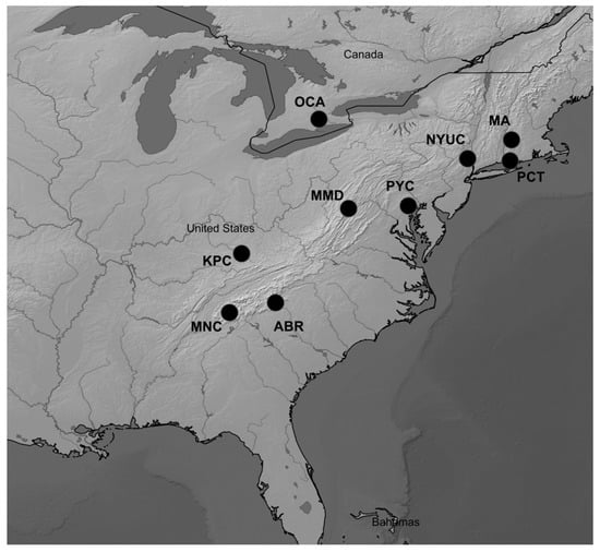
Figure 1.
Locations of the sampled chestnut populations, OCA—Ontario, MA—Massachusetts, PCT—Portland, NYUC—New York, PYC—Pennsylvania, MMD—Maryland, KPC—Kentucky, ABR—Asheville, MNC—Murphy; the map was created with SimpleMappr [21].

Table 1.
Population characteristics.
Climate data (19 bioclimatic variables “bioclim”, period 1950–2000, resolution: 30 arc sec) for the sampling sites were obtained from the WorldClim database [22] using the Data Extraction Tool of the Senckenberg Research Society (http://dataportal-senckenberg.de/dataExtractTool/). Based on the WorldClim data, two additional variables were calculated that may be important for adaptation in tree species: mean growing season temperature and mean growing season precipitation, where the growing season was considered to last from May 1 to 30 September. The former ranged from 16.5 °C for the Maryland population to 21 °C for the Kentucky population, whereas the latter ranged from 404 mm (Ontario population) to 628 mm (Asheville population) (Table 1). An overview of all environmental variables can be found in Table S1.
2.2. SSR Genotyping
Populations were characterized at a total of 24 SSRs (17 EST-SSRs and 7 g-SSRs; Table S2). All markers (except for QaCA022) were used for genetic mapping in C. mollissima [11], and cover 10 different linkage groups (LGs) (Table S2). Genotype data for the 17 EST-SSRs were obtained from a previous study [16]. The EST-SSRs were originally developed in C. mollissima [11]. In order to have a better representation of putatively neutral genetic variation, further genotyping was conducted for the remaining seven g-SSRs. Six of these g-SSRs were originally developed for Castanea sativa (CsCAT1, CsCAT3, CsCAT7, CsCAT8, CsCAT14 and CsCAT24) and one (QaCA022) was originally derived from Quercus alba but successfully tested in Castanea dentata [17]. For cost-efficient PCR, a M13-specific sequence (5′-CACGACGTTGTAAACGAC-3′) was added to the 5′ end of each forward primer, so that only the M13 primer had to be labeled with fluorescent dyes [11,23]. For more accurate genotyping we further added a PIG-tail sequence (5′-GTTTCTT-3′) to the 5′ end of each reverse primer [24]. The primer CsCAT24 was analyzed in a separate PCR, while for the other primers multiplex reactions were established and analyzed (multiplex 1: CsCAT8 and CsCAT14; multiplex 2: CsCAT3 and QaCA022; and multiplex 3: CsCAT1 and CsCAT7). A touchdown PCR program comprised of the following steps was used for all reactions: an initial denaturation of 95 °C for 15 min, followed by 10 touchdown cycles of 94 °C for 1 min, 60 °C (−1 °C per cycle) for 1 min, and 72 °C for 1 min, 25 cycles of 94 ° for 1 min, 50 °C for 1 min, and 72 °C for 1 min, followed by a final extension step of 72 °C for 20 min. The PCR mix consisted of 1µL DNA (ca. 0.6 ng/µL), 1.5 µL 10x reaction buffer B (Solis BioDyne, Tartu, Estonia), 1.5 µL MgCl2 (25 mM), 1 µL dNTPs (2.5 mM each dNTP), 0.2 µL (5 U/µL) HOT FIREPol Taq DNA polymerase (Solis BioDyne, Tartu, Estonia), 0.2 µL (5 picomole/µL) tailed forward primer, 0.5 µL (5 picomole/µL) PIG-tailed reverse primer, 1 µL (5 picomole/µL) dye labeled (6-FAM or 6-HEX) M13 primer and 5.5 µL H2O. Fragments were separated on an ABI 3130xl Genetic Analyzer (Applied Biosystems, Foster City, CA, USA) using GS 500 ROX (Applied Biosystems, Foster City, CA, USA) as an internal size standard. Microsatellite genotyping was conducted with the GeneMapper 4.0 software (Applied Biosystems, Foster City, CA, USA). All genotypic data can be found in data file S1.
2.3. Data Analysis
A principle component analysis (PCA) was conducted on the climate variables to obtain principle components (PCs) for the association analysis (see below). In addition to the 19 bioclim variables, longitude, latitude, altitude, mean growing season temperature, and mean growing season precipitation were included in the analysis. The PCA was performed with the “prcomp” function in R 3.4.3 [25]. For the PCA the variables were standardized to a mean of 0 and a standard deviation of 1. For an interpretation of the PCs we calculated Spearman’s rank correlation coefficients among environmental variables and PCs using the “corr.test” function in the psych 1.7.8 R package [26] with correction for multiple testing (false discovery rate (FDR) [27] with a threshold of 5%).
The GenAlEx 6.5 software [28,29] was used to calculate the number of alleles (Na), the mean number of private alleles (Pa), the observed heterozygosity (Ho), and the expected heterozygosity (He) separately for the seven g-SSRs and the 17 EST-SSRs as well as across all markers. The inbreeding coefficient (FIS) [30] and linkage disequilibrium (LD) were calculated with the Genepop software 4.7 [31] using 10,000 demorizations, 100 batches and 5000 iterations per batch for Markov chain parameters. Presence and frequency of null alleles were determined with the Micro-Checker software 2.2.3 [32]. Population structure was inferred with the STRUCTURE 2.3.4 software [33]. Two different analyses were performed: the first one based on the complete marker set, and the second one based only on potentially neutral SSR markers (markers CmSI0495, CmSI0527, CmSI0537, CmSI0559, CmSI0561, CmSI0608, CmSI0611, CsCAT7 and CsCAT24). Markers were considered as neutral when they did not show deviations from neutrality in the outlier analyses, and when they were not associated with the PCs based on the environmental variables (see below). For both analyses, the admixture model and correlated allele frequencies were selected. A burn-in period of 50,000 and Markov chain Monte Carlo (MCMC) replicates of 100,000 were used. Potential clusters (K) from 1 to 16 were tested using 10 iterations. The Δ K method by Evanno et al. [34] was applied to determine the most likely number of K using the STRUCTURE HARVESTER 0.6.94 program [35]. The CLUMPAK software [36] was used for summation and graphical representation of the STRUCTURE results.
Outlier analyses were conducted for all loci using LOSITAN 1.0 [37] with 70,000 simulations, a FDR of 0.1, and the stepwise mutation model. Additionally, the BayeScan software 2.1 [38] was used to detect outlier loci. We used default parameters including 100,000 iterations after a burn-in of 50,000. A q-value threshold of 10% was applied to determine significant outliers. The markers used in this study were not directly derived from Castanea dentata. Therefore, sequences in which the outlier loci and loci that were significantly associated with the PCs of the environmental variables (see results) were located, were used for sequence similarity searches against Castanea dentata transcripts using the BLAST search option on the hardwood genomics homepage (https://www.hardwoodgenomics.org/blast).
A general linear model (GLM) implemented in the TASSEL 2.1 software [39] was used to detect marker-environment associations. In association studies, it is necessary to account for neutral population structure [40]. The outlier analysis revealed not only significant EST-SSRs, but also two significant g-SSR loci (see below). Furthermore, loci under weak selection may not be detected by outlier approaches [40,41]. Thus, in the final association analysis only markers without signatures of selection in the outlier and initial association analyses (see below) were used to infer neutral population structure. Initially, only populations among which no population structure was detected using all markers were included in the association analyses (analysis 1: Ontario, Maryland, Kentucky, Asheville and Murphy; analysis 2: Massachusetts, New York and Portland), and hence, no Q-matrix was used as covariate in the model to correct for population structure. Tested were associations between all markers and the first three PCs (PC1, PC2 and PC3) obtained from the PCA of the environmental variables. In the final association analysis, loci that showed significant associations in the initial analyses and outlier loci were tested for associations with the three PCs in all populations. The remaining neutral loci were used to calculate the Q-matrix in STRUCTURE as covariate to account for population structure. The reported p-values are based on 1000 permutations and correction for multiple testing based on the methods by Churchill and Doerge [42] and Ge et al. [43] implemented in the TASSEL software.
3. Results
3.1. Environmental Variables
The PCA showed that the first three PCs (hereafter PC1, PC2 and PC3) had eigenvalues higher than 1 and explained 92.01% of the variance of the environmental variables. For a better interpretation of the different PCs, they were correlated with the environmental variables. PC1 showed a significant negative correlation with latitude, temperature seasonality (bio4), and temperature annual range (bio7), but also a positive correlation with several climatic variables such as annual mean temperature (bio1), minimum temperature of the coldest month (bio6), or annual precipitation (bio12) (Table 2). PC2 was significantly positively correlated with the maximum temperature of the warmest month (bio5), and PC3 was significantly negatively correlated with altitude.
Table 2.
Correlation between principal components and environmental variables.
3.2. Genetic Diversity and Population Structure
The number of alleles (Na) ranged from 4.1 in the Portland population to 7.3 in the Murphy population, and the mean number of private alleles ranged from 0 (Portland) to 0.833 (Murphy) (Table 3). The observed heterozygosity (Ho) ranged from 0.521 (Kentucky) to 0.586 (Murphy), whereas the expected heterozygosity (He) ranged from 0.469 (Portland) to 0.610 (Murphy). The mean fixation index (FIS) was 0.0157 and it was significantly different from zero in six populations (Table 3), albeit no population showed consistently positive or negative FIS values for all markers (Table S3). The mean genetic diversity indices (except Pa) were lower based on EST-SSRs than on g-SSRs (Table 3), even though several EST-SSRs also showed high values of Na, Ho and He (Table 4). The percentage of loci pairs in linkage disequilibrium ranged from 2.5% in the New York population to 9.8% in the Kentucky population, with a mean of 5.6% among all populations (Table S4). Only few markers showed evidence for the presence of null-alleles in the different populations (Table S5).
Table 3.
Genetic diversity indices.
Table 4.
Genetic diversity indices for each marker over all populations.
The STRUCTURE analysis revealed the most likely number of K = 2 based on the ΔK method [34] and the complete marker set, and the most likely number of K = 3 based on only potentially neutral markers (Figure S1). Based on the complete marker set, the northeastern populations Massachusetts, New York and Portland formed one cluster, and the remaining populations a second cluster (Figure 2). Only the Pennsylvania population was not clearly assigned to one of the two clusters, but reveals a high degree of admixture. Based on potentially neutral loci, a similar clustering was observed, albeit the Pennsylvania population showed a similar admixture level as the southern populations and Ontario (Figure S2).
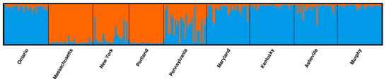
Figure 2.
Clustering of individuals based on the complete marker set.
3.3. Outlier and Environmental Association Analysis
The LOSITAN analysis revealed five outlier loci that showed higher FST values than expected under neutral assumptions (CsCAT1, CsCAT3, CmSI0031, CmSI0600, and CmSI0594). With BayeScan no significant outlier loci were detected.
Association analysis 1, in which the populations from Ontario, Maryland, Kentucky, Asheville, and Murphy (second cluster as identified by STRUCTURE) were included, revealed 8 loci significantly associated with at least one of the PCs (Table S6), whereas association analysis 2, in which the populations from Massachusetts, New York, and Portland (first cluster) were included, revealed 11 significant loci (Table S6). A total of nine markers revealed no signatures of selection in the outlier and initial association analyses and were used to calculate the Q-matrix as covariate to be used in the final association analysis based on all populations. In this analysis, 10 significant loci were found, including the loci that were also significant in the outlier analysis (Table 5).
Table 5.
SSR markers significantly associated with principal components.
The phenotypic variation explained by markers (R2) ranged from 0.014 for marker CmSI0594 to 0.45 for marker CsCAT3, and was on average higher for markers significantly associated with the PCs than for non-significant markers (Figure 3). In total, 7 of the 10 significant loci were successfully assigned to Castanea dentata transcripts using BLAST against the C. dentata UniGene-transcript database (Table S7).
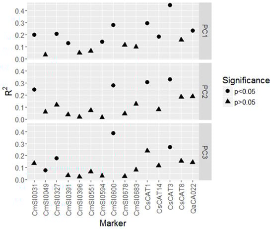
Figure 3.
Phenotypic variation explained by markers (R2). Filled circles represent markers that are significantly associated with the respective PC.
4. Discussion
Seven g-SSRs were used to complement EST-SSR-based genotypic data of nine American chestnut populations sampling the native range that were previously investigated by Gailing and Nelson [16]. Compared to the EST-SSRs, g-SSRs revealed higher genetic diversity values (Na, Ho, He), which was expected due to the usually higher variability of the latter marker type [44]. Only the mean number of private alleles (Pa) was higher for EST-SSRs. These private alleles may present adaptive beneficial variants, but this remains open. The reported distribution of genetic variation among the analyzed populations by Gailing and Nelson [16] could be confirmed with both the newly applied g-SSRs and the complete marker set (g-SSRs and EST-SSRs): populations from further south as well as the Ontario population in Canada showed a higher allelic diversity than populations further northeast in the USA. Furthermore, FIS values were positive for (south) western populations and negative for northeastern populations. One exception was the Massachusetts population that showed a significantly positive FIS value based on g-SSRs, while the FIS value was not significantly different from zero based on EST-SSRs. Also the population structure among populations was similar to that revealed by Gailing and Nelson [16]. The northeastern populations of Massachusetts, New York and Portland formed one cluster and the remaining populations a second cluster. Only the Pennsylvania population reveals a high level of admixture between both clusters. Since all SSR-markers were transferred from related tree species, we tested for the presence of null alleles. Only a few SSRs showed evidence for null alleles in the populations (Table S5), and hence, did likely not bias the results of our study. Further, only 5.6% of marker pairs were found to be in LD among all populations. This could be expected, since the markers have previously been mapped to 10 different LGs in C. mollissma [11].
The outlier analysis based on the Fdist approach [45] implemented in the LOSITAN software [37] revealed five outlier loci, whereas no outlier loci were detected with a Bayesian method implemented in the BayeScan software [38]. BayeScan has been shown to be more conservative in detecting outliers compared to other methods before [46,47,48].
All five FST-outlier loci were significantly associated with PC1, four with PC2 and only two with PC3. Additionally, five more loci were associated with at least one of the PCs. The phenotypic variation explained by markers (R2) was higher for significant loci (in the outlier and association analysis; R2: 0.08 to 0.45, mean of 0.25) compared to neutral loci (R2: 0.01 to 0.24, mean 0.09). The R2 values were relatively high and at the top end of other reported values for tree species summarized in Lind et al. [49]. In association analyses, population structure can lead to spurious associations [50]. Therefore, neutral population structure is usually included as a covariate in models searching for significant marker-trait associations. Likewise, population structure based on potentially neutral markers was considered in our association analysis, but with our marker set it was challenging to reliably identify neutral loci. Since PC1 was significantly correlated with several environmental variables, but also with latitude, the associations of markers with PC1 may be biased by population structure related to geography. PC2, however, was only correlated with bio5 (maximum temperature of the warmest month), and PC3 was only (negatively) correlated with altitude. Hence, loci associated with these two PCs may indeed be involved in adaptive processes related to environmental conditions. In total, four of the six loci that were associated with PC2 and PC3 were also significant in the FST-outlier analysis, and hence, detected by two different approaches. Therefore, the four loci CmSI0031 (LG_H, 25.3 cM), CmSI0600 (LG_J, 55.4 cM), CsCAT1 (LG_C; ~45.7 cM), and CsCAT3 (LG_J; ~39.0 cM) [11,51] might be the most promising ones for further analyses. Loci CsCAT1 and CsCAT3 are g-SSRs originally developed in C. sativa. Usually, g-SSRs are located within non-coding genomic regions, and hence, they are likely not directly involved in adaptive processes, but rather linked with loci under selection. Locus CsCAT1, however, was successfully assigned to a Castanea dentata transcript (AC454_contig17130_v3; uncharacterized protein) using BLAST (Table S7). Thus, this locus might be located next to or within a coding region, and therefore be directly involved in adaptive processes. Also the other two loci were successfully assigned to C. dentata transcripts: locus CmSI0031 showed similarities with the transcript “AC454_contig35613_v3,” which shows homology to a Tubulin alpha chain, and locus CmSI0600 was assigned to transcript “AC454_contig7150_v3,” for which no specific protein could be inferred (“uncharacterized protein”). Thus, the specific function of the genes, in which the outliers are located, remains open. Nevertheless, PC2 and PC3 are almost exclusively related to the maximum temperature of the warmest month or altitude. Hence, the loci associated with these PCs may be involved in temperature-related adaptive processes. Temperature can play an important role in the performance and adaptation of American chestnut provenances. For instance, C. dentata growth was (among others) negatively correlated with previous year August temperature [52]. In addition, Schaberg et al. [53] showed that height growth was correlated with winter shoot injury. In general, American chestnut is vulnerable to winter injury in its northern distribution area [15], and provenances differ in cold hardiness [53,54].
5. Conclusions
The wider genomic coverage represented by the enlarged marker set compared to Gailing and Nelson [16] revealed similar distribution patterns of genetic diversity and differentiation among the populations. By means of outlier and environmental association analysis, ten markers were identified that are significantly associated with environmental variables of the population sites. Four of these markers are of particular interest and could be involved in temperature-related adaptive processes in American chestnut. Future studies may take advantage of genomic resources that have recently been developed for chestnut species [10,11,13,14] to get a better understanding of adaptation patterns in C. dentata.
Supplementary Materials
The following are available online at http://www.mdpi.com/1999-4907/9/11/695/s1, Data file S1: Genotypic data, Figure S1: Plots of delta K and log likelihood for each K based on the complete marker set (a), and potentially neutral markers that did not show deviations from neutrality in the outlier analysis (b), Figure S2: Clustering of individuals for K = 3 based on potentially neutral markers, Table S1: Environmental variables of the analyzed populations, Table S2: Primer information, Table S3: FIS values of the SSR markers in the different populations, Table S4: Percentage of SSR pairs with significant linkage disequilibrium, p < 0.05, Table S5: Frequency of null alleles, Table S6: SSR-markers significantly associated with principal components within the two different population clusters (a) Ontario, Maryland, Kentucky, Asheville, and Murphy; (b) Massachusetts, New York, and Portland, Table S7: BLAST results and linkage groups of the loci significantly associated with the environmental variables.
Author Contributions
Conceptualization, O.G. and C.D.N.; methodology, M.M. and O.G.; validation, M.M., O.G. and C.D.N.; formal analysis, M.M.; investigation, M.M.; resources, O.G. and C.D.N.; data curation, M.M.; writing—original draft preparation, M.M.; writing—review and editing, M.M., O.G. and C.D.N.; visualization, M.M.; supervision, O.G.; project administration, O.G.; funding acquisition, O.G. and C.D.N.
Funding
This research was partly funded by The American Chestnut Foundation.
Acknowledgments
We thank Christine Radler for help with the lab work.
Conflicts of Interest
The authors declare no conflict of interest. The funders had no role in the design of the study; in the collection, analyses, or interpretation of data; in the writing of the manuscript, or in the decision to publish the results.
References
- Jacobs, D.F.; Dalgleish, H.J.; Nelson, C.D. A conceptual framework for restoration of threatened plants: The effective model of American chestnut (Castanea dentata) reintroduction. New Phytol. 2013, 197, 378–393. [Google Scholar] [CrossRef] [PubMed]
- Ellison, A.M.; Bank, M.S.; Clinton, B.D.; Colburn, E.A.; Elliott, K.; Ford, C.R.; Foster, D.R.; Kloeppel, B.D.; Knoepp, J.D.; Lovett, G.M.; et al. Loss of foundation species: Consequences for the structure and dynamics of forested ecosystems. Front. Ecol. Environ. 2005, 3, 479–486. [Google Scholar] [CrossRef]
- Anagnostakis, S.L. The effect of multiple importations of pests and pathogens on a native tree. Biol. Invasions 2001, 3, 245–254. [Google Scholar] [CrossRef]
- Kubisiak, T.L.; Hebard, F.V.; Nelson, C.D.; Zhang, J.; Bernatzky, R.; Huang, H.; Anagnostakis, S.L.; Doudrick, R.L. Molecular mapping of resistance to blight in an interspecific cross in the genus Castanea. Phytopathology 1997, 87, 751–759. [Google Scholar] [CrossRef] [PubMed]
- Milgroom, M.G.; Cortesi, P. Biological control of chestnut blight with hypovirulence: A critical analysis. Annu. Rev. Phytopathol. 2004, 42, 311–338. [Google Scholar] [CrossRef] [PubMed]
- Merkle, S.A.; Andrade, G.M.; Nairn, C.J.; Powell, W.A.; Maynard, C.A. Restoration of threatened species: A noble cause for transgenic trees. Tree Genet. Genomes 2007, 3, 111–118. [Google Scholar] [CrossRef]
- Hebard, F. The backcross breeding program of the American Chestnut Foundation. J. Am. Chestnut Found. 2005, 19, 55–77. [Google Scholar]
- Bauman, J.M.; Keiffer, C.H.; McCarthy, B.C. Growth performance and chestnut blight incidence (Cryphonectria parasitica) of backcrossed chestnut seedlings in surface mine restoration. New For. 2014, 45, 813–828. [Google Scholar] [CrossRef]
- Clark, S.L.; Schlarbaum, S.E.; Saxton, A.M.; Hebard, F.V. Establishment of American chestnuts (Castanea dentata) bred for blight (Cryphonectria parasitica) resistance: Influence of breeding and nursery grading. New For. 2016, 47, 243–270. [Google Scholar] [CrossRef]
- Barakat, A.; Staton, M.; Cheng, C.H.; Park, J.; Yassin, N.B.; Ficklin, S.; Yeh, C.C.; Hebard, F.; Baier, K.; Powell, W.; et al. Chestnut resistance to the blight disease: Insights from transcriptome analysis. BMC Plant Biol. 2012, 12, 38. [Google Scholar] [CrossRef] [PubMed]
- Kubisiak, T.L.; Nelson, C.D.; Staton, M.E.; Zhebentyayeva, T.; Smith, C.; Olukolu, B.A.; Fang, G.C.; Hebard, F.V.; Anagnostakis, S.; Wheeler, N.; et al. A transcriptome-based genetic map of Chinese chestnut (Castanea mollissima) and identification of regions of segmental homology with peach (Prunus persica). Tree Genet. Genomes 2013, 9, 557–571. [Google Scholar] [CrossRef]
- Bodénès, C.; Chancerel, E.; Gailing, O.; Vendramin, G.G.; Bagnoli, F.; Durand, J.; Goicoechea, P.G.; Soliani, C.; Villani, F.; Mattioni, C.; et al. Comparative mapping in the Fagaceae and beyond with EST-SSRs. BMC Plant Biol. 2012, 12, 153. [Google Scholar] [CrossRef] [PubMed]
- Staton, M.; Zhebentyayeva, T.; Olukolu, B.; Fang, G.C.; Nelson, D.; Carlson, J.E.; Abbott, A.G. Substantial genome synteny preservation among woody angiosperm species: Comparative genomics of Chinese chestnut (Castanea mollissima) and plant reference genomes. BMC Genom. 2015, 16, 744. [Google Scholar] [CrossRef] [PubMed]
- Cheng, L.; Huang, W.; Lan, Y.; Cao, Q.; Su, S.; Zhou, Z.; Wang, J.; Liu, J.; Hu, G. The complete chloroplast genome sequence of the wild Chinese chestnut (Castanea mollissima). Conserv. Genet. Resour. 2017. [Google Scholar] [CrossRef]
- Gurney, K.M.; Schaberg, P.G.; Hawley, G.J.; Shane, J.B. Inadequate cold tolerance as a possible limitation to American chestnut restoration in the Northeastern United States. Restor. Ecol. 2011, 19, 55–63. [Google Scholar] [CrossRef]
- Gailing, O.; Nelson, C.D. Genetic variation patterns of American chestnut populations at EST-SSRs. Botany 2017, 95, 799–807. [Google Scholar] [CrossRef]
- Kubisiak, T.L.; Roberds, J.H. Genetic Structure of American Chestnut Populations Based on Neutral DNA Markers; U.S. Department of the Interior, National Park Service, National Capital Region, Center for Urban Ecology: Washington, DC, USA, 2006.
- Huang, H.; Dane, F.; Kubisiak, T.L. Allozyme and RAPD analysis of the genetic diversity and geographic variation in wild populations of the American chestnut (Fagaceae). Am. J. Bot. 1998, 85, 1013–1021. [Google Scholar] [CrossRef] [PubMed]
- Davis, M.B. Quaternary history of deciduous forests of eastern North America and Europe. Ann. Mo. Bot. Gard. 1983, 70, 550–563. [Google Scholar] [CrossRef]
- Li, X.; Dane, F. Comparative chloroplast and nuclear DNA analysis of Castanea species in the southern region of the USA. Tree Genet. Genomes 2012, 9, 107–116. [Google Scholar] [CrossRef]
- Shorthouse, D. SimpleMappr, an Online Tool to Produce Publication-Quality Point Maps. Available online: http://www.simplemappr.net (accessed on 27 April 2018).
- Hijmans, R.J.; Cameron, S.E.; Parra, J.L.; Jones, P.G.; Jarvis, A. Very high resolution interpolated climate surfaces for global land areas. Int. J. Climatol. 2005, 25, 1965–1978. [Google Scholar] [CrossRef]
- Schuelke, M. An economic method for the fluorescent labeling of PCR fragments. Nat. Biotechnol. 2000, 18, 233–234. [Google Scholar] [CrossRef] [PubMed]
- Brownstein, M.J.; Carpten, J.D.; Smith, J.R. Modulation of non-templated nucleotide addition by Taq DNA polymerase: Primer modifications that facilitate genotyping. BioTechniques 1996, 20, 1004–1006, 1008–1010. [Google Scholar] [CrossRef] [PubMed]
- R Core Team. R: A Language and Environment for Statistical Computing. Available online: http://www.R-project.org/ (accessed on 2 July 2018).
- Revelle, W. Psych: Procedures for Personality and Psychological Research. Available online: https://CRAN.R-project.org/package=psych (accessed on 31 October 2018).
- Benjamini, Y.; Hochberg, Y. Controlling the false discovery rate: A practical and powerful approach to multiple testing. J. R. Stat. Soc. Ser. B Methodol. 1995, 57, 289–300. [Google Scholar]
- Peakall, R.; Smouse, P.E. Genalex 6: Genetic analysis in Excel. Population genetic software for teaching and research. Mol. Ecol. Notes 2006, 6, 288–295. [Google Scholar] [CrossRef]
- Peakall, R.; Smouse, P.E. GenAlEx 6.5: Genetic analysis in Excel. Population genetic software for teaching and research—An update. Bioinformatics 2012, 28, 2537–2539. [Google Scholar] [CrossRef] [PubMed]
- Weir, B.S.; Cockerham, C.C. Estimating F-statistics for the analysis of population structure. Evolution 1984, 38, 1358–1370. [Google Scholar] [CrossRef] [PubMed]
- Rousset, F. Genepop’007: A complete re-implementation of the genepop software for Windows and Linux. Mol. Ecol. Resour. 2008, 8, 103–106. [Google Scholar] [CrossRef] [PubMed]
- Van Oosterhout, C.; Hutchinson, W.F.; Wills, D.P.M.; Shipley, P. Micro-checker: Software for identifying and correcting genotyping errors in microsatellite data. Mol. Ecol. Notes 2004, 4, 535–538. [Google Scholar] [CrossRef]
- Pritchard, J.K.; Stephens, M.; Donnelly, P. Inference of population structure using multilocus genotype data. Genetics 2000, 155, 945–959. [Google Scholar] [PubMed]
- Evanno, G.; Regnaut, S.; Goudet, J. Detecting the number of clusters of individuals using the software STRUCTURE: A simulation study. Mol. Ecol. 2005, 14, 2611–2620. [Google Scholar] [CrossRef] [PubMed]
- Earl, D.A.; vonHoldt, B.M. STRUCTURE HARVESTER: A website and program for visualizing STRUCTURE output and implementing the Evanno method. Conserv. Genet. Resour. 2012, 4, 359–361. [Google Scholar] [CrossRef]
- Kopelman, N.M.; Mayzel, J.; Jakobsson, M.; Rosenberg, N.A.; Mayrose, I. CLUMPAK: A program for identifying clustering modes and packaging population structure inferences across K. Mol. Ecol. Resour. 2015, 15, 1179–1191. [Google Scholar] [CrossRef] [PubMed]
- Antao, T.; Lopes, A.; Lopes, R.J.; Beja-Pereira, A.; Luikart, G. LOSITAN: A workbench to detect molecular adaptation based on a Fst-outlier method. BMC Bioinform. 2008, 9, 323. [Google Scholar] [CrossRef] [PubMed]
- Foll, M.; Gaggiotti, O. A genome-scan method to identify selected loci appropriate for both dominant and codominant markers: A Bayesian perspective. Genetics 2008, 180, 977–993. [Google Scholar] [CrossRef] [PubMed]
- Bradbury, P.J.; Zhang, Z.; Kroon, D.E.; Casstevens, T.M.; Ramdoss, Y.; Buckler, E.S. TASSEL: Software for association mapping of complex traits in diverse samples. Bioinformatics 2007, 23, 2633–2635. [Google Scholar] [CrossRef] [PubMed]
- Rellstab, C.; Gugerli, F.; Eckert, A.J.; Hancock, A.M.; Holderegger, R. A practical guide to environmental association analysis in landscape genomics. Mol. Ecol. 2015, 24, 4348–4370. [Google Scholar] [CrossRef] [PubMed]
- Narum, S.R.; Hess, J.E. Comparison of FST outlier tests for SNP loci under selection. Mol. Ecol. Resour. 2011, 11, 184–194. [Google Scholar] [CrossRef] [PubMed]
- Churchill, G.A.; Doerge, R.W. Empirical threshold values for quantitative trait mapping. Genetics 1994, 138, 963–971. [Google Scholar] [PubMed]
- Ge, Y.; Dudoit, S.; Speed, T.P. Resampling-based multiple testing for microarray data analysis. Test 2003, 12, 1–77. [Google Scholar] [CrossRef]
- Ellis, J.R.; Burke, J.M. EST-SSRs as a resource for population genetic analyses. Heredity 2007, 99, 125. [Google Scholar] [CrossRef] [PubMed]
- Beaumont, M.A.; Nichols, R.A. Evaluating loci for use in the genetic analysis of population structure. Proc. R. Soc. B Biol. Sci. 1996, 263, 1619–1626. [Google Scholar] [CrossRef]
- Zhan, X.; Dixon, A.; Batbayar, N.; Bragin, E.; Ayas, Z.; Deutschova, L.; Chavko, J.; Domashevsky, S.; Dorosencu, A.; Bagyura, J.; et al. Exonic versus intronic SNPs: Contrasting roles in revealing the population genetic differentiation of a widespread bird species. Heredity 2015, 114, 1–9. [Google Scholar] [CrossRef] [PubMed]
- Henry, P.; Russello, M.A. Adaptive divergence along environmental gradients in a climate-change-sensitive mammal. Ecol. Evol. 2013, 3, 3906–3917. [Google Scholar] [CrossRef] [PubMed]
- Huang, K.; Whitlock, R.; Press, M.C.; Scholes, J.D. Variation for host range within and among populations of the parasitic plant Striga hermonthica. Heredity 2012, 108, 96–104. [Google Scholar] [CrossRef] [PubMed]
- Lind, B.M.; Menon, M.; Bolte, C.E.; Faske, T.M.; Eckert, A.J. The genomics of local adaptation in trees: Are we out of the woods yet? Tree Genet. Genomes 2018, 14. [Google Scholar] [CrossRef]
- Lander, E.; Schork, N. Genetic dissection of complex traits. Science 1994, 265, 2037–2048. [Google Scholar] [CrossRef] [PubMed]
- Marinoni, D.; Akkak, A.; Bounous, G.; Edwards, K.J.; Botta, R. Development and characterization of microsatellite markers in Castanea sativa (Mill.). Mol. Breed. 2003, 11, 127–136. [Google Scholar] [CrossRef]
- McEwan, R.W.; Keiffer, C.H.; McCarthy, B.C. Dendroecology of American chestnut in a disjunct stand of oak–chestnut forest. Can. J. For. Res. 2006, 36, 1–11. [Google Scholar] [CrossRef]
- Schaberg, P.G.; Saielli, T.M.; Hawley, G.J.; Halman, J.M.; Gurney, K.M. Winter Injury of American Chestnut Seedlings Grown in A Common Garden at The Species’ Northern Range Limit; Miller, G.W., Schuler, T.M., Gottschalk, K.W., Brooks, J.R., Grushecky, S.T., Spong, B.D., Rentch, J.S., Eds.; U.S. Department of Agriculture, Forest Service, Northern Research Station: Morgantown, WV, USA, 2013; pp. 72–79.
- Saielli, T.M.; Schaberg, P.G.; Hawley, G.J.; Halman, J.M.; Gurney, K.M. Nut cold hardiness as a factor influencing the restoration of American chestnut in northern latitudes and high elevations. Can. J. For. Res. 2012, 42, 849–857. [Google Scholar] [CrossRef]
© 2018 by the authors. Licensee MDPI, Basel, Switzerland. This article is an open access article distributed under the terms and conditions of the Creative Commons Attribution (CC BY) license (http://creativecommons.org/licenses/by/4.0/).