
Characterizing Habitat Elements and Their Distribution over Several Spatial Scales: The Case of the Fisher

1
Department of Geography, University of California, Santa Barbara, CA 93106, USA
2
U.S. Forest Service, Land Management Planning, San Francisco, CA 94111, USA
*
Author to whom correspondence should be addressed.
Forests 2017, 8(6), 186; https://doi.org/10.3390/f8060186
Submission received: 11 February 2017
/
Revised: 20 May 2017
/
Accepted: 24 May 2017
/
Published: 28 May 2017
(This article belongs to the Special Issue Management Strategies for Forest Ecosystem Services)
Abstract
:In past studies of the fisher (Pekania pennanti) most researchers have concluded that fisher habitat must consist of mostly mature to late-seral forest with few, if any, openings. Without doubt, certain elements found in mature to late-seral forests are required by females to successfully rear their young, but some recent work casts doubt on the extent that a continuous canopy of tree coverage and a preponderance of older stands are necessary as long as certain components exist. This paper explores this issue with an attempt to better characterize essential elements of habitat for the female fisher. This characterization is based upon fine-scale inventory plot data that is analyzed across several spatial scales that represent a small neighborhood about den sites, the forest of the 75% kernel density estimate for female home ranges, and the forested region as a whole. We present results of a test of significance in comparing habitat elements across these three scales. Our findings suggest that certain habitat elements typically found in mature to late seral forests must be present at a certain fraction of the landscape for the fisher. The approach described here may be of considerable value in developing guidelines for conservation agreements.
1. Introduction
One of the biggest challenges facing conservation biologists and ecologists is the development of a knowledge base that is sufficient to make cogent management decisions in protecting threatened species. Often, expert opinion is used to address the key question: What comprises suitable habitat for key species and how large an area is necessary? Such opinion, and even modeling, tends to support what is commonly known but does not always capture needed spatial composition. For example, the ideal habitat of the San Joaquin Kit Fox (Vulpes macrotis mutica) is a grassy plain that has not been plowed or cultivated and tends to avoid riparian areas. Conventional wisdom suggests that they would avoid urban areas as they would end up as road kill [1,2,3,4,5]. However, the kit fox has recently been found in sizable numbers living in urban areas [6], including the town of Bakersfield, CA—burrowing under portable school buildings, hunting on school grounds and even eating the leftovers from McDonald’s and other fast food restaurants [7]. One might then ask oneself, “What is wrong with this picture?” The Kit Fox is doing what expert opinion had once thought impossible: living in an urban area. However, upon a closer look at school grounds, one can see habitat elements that were less understood, but are now brought into better focus. There are large open grassy spaces, protected den areas under portable classrooms, food sources such as mice, squirrels, etc. within easy reach, and quiet school grounds at night. Thus, some of the key habitat elements exist in an urban area for the Kit Fox.
How a species uses or avoids a landscape is dependent upon the distribution and spatial configuration of habitat elements within it. Significant habitat elements are typically ascertained based upon a species recurrent use of a landscape feature, usually constructed as a landscape classification. For instance, if a species is found to den in large trees with cavities such as the fisher (Pekania pennanti; formerly Martes pennanti [8]), and trees with cavities tend to be in forest classes consisting of mature to late-seral forest [9], there is a tendency to include this classification (mature to late-seral stands) as the requisite for habitat, rather than understanding the needed distribution of such structures. This is partly due to the fact that large trees with cavities (structure trees) are certain to exist in mature forest classes. However, a scattering of older structure trees with cavities over a more heterogeneous landscape containing younger stands on the average could be just as suitable as those that are homogeneous and old. Thus, broad habitat characterizations by experts should be tested in a manner for which habitat significance may be assessed [10]. Understanding that mature to late seral stand elements are necessary, has significant implications for forest management (for example, thinning and removing fuels for promoting fire resilience [11]).
This paper proposes a statistical framework to identify significant structural components (like large trees) and their distribution within the landscape to help support such management implications. An evaluation procedure, which we call k-Max-l, is developed in conjunction with the well-known Kolmogorov-Smirnov significance test as an indicator function to evaluate habitat element distribution across several spatial scales. We apply this approach as a means to better characterize the needs of female fishers during the spring to early summer denning season, a critical time for successful reproduction. In the next section we describe our study area, the fisher, and the three spatial scales of analysis.
2. Study Area and Methods
2.1. The Forest, the Fisher and the Three Scales of Our Modeling Effort
The objective of our study was to characterize the spatial distribution of important structures for the fisher (Pekania pennanti [8]) in an interior northern California forest. The forested study area lies within the center-east portion of Trinity County, California (Figure 1), and represents approximately 182 km2 (45,000 acres). Of this total, 78% is private industrial timberland, 15% lies within Shasta-Trinity national forest, and 7% is held by private non-industrial landowners. The location and the size of the study area is like that analyzed in Buck et al. [12], though the level of public-private ownership is reversed. The forest is a mixed conifer-hardwood forest consisting of Douglas-fir (Psuedotsuga menziesii), ponderosa pine (Pinus ponderosa), incense-cedar (Calocedrus decurrens), white fir (Abies concolor), black oak (Quercus kelloggii) and canyon live oak (Quercus chrysolepis). This forest is heterogeneous in the sense that the forest consists of smaller younger conifer and hardwood trees, with scattered individuals or groups of much larger conifer or hardwood trees, with many forest openings. The forest has generally low biomass volume per acre and the average basal area per acre in trees >20.32 cm (>8 inches) diameter at breast height (dbh) is 24.105 m2 per hectare (105 ft2 per acre) for conifers and 10.331 m2 per hectare (45 ft2 per acre) for hardwoods. Some of the hardwood trees are >40.64 cm (>16 inches) dbh and have grown and persisted in areas where conifers were logged. This variation is due to logging activity conducted in the 1950’s and 1970s, several wildfires that burned into the area in 1964, 1974, 1991, and 1992, and severe weather events (hail and wind) that denuded some of the trees.
This forest area has been inventoried with 10,615 fine scale sample plots by Sierra Pacific Industries. The resultant inventory plot data set was collected in 2006 by registered professional foresters and generated using an angle gauge and variable plot cruising. The angle gauge was used to identify trees to include and collect attribute information on, for each sample plot. The data set is a systematic sample with a random starting point. The plot dataset consists of 10,615 unique plot points containing several attributes (Table 1 for a sample of measured attributes). Aggregate measures, such as basal area of conifers and basal area of hardwoods includes all species of that type. Plot points are generally established every 80.4672 m (264 ft) along North-South transects, which are systematically spaced every 201.1680 m (660 ft) in East-West transects. The plot sampling design was established such that there is a plot sample for approximately every 1.61874 ha (4 acres, 80.4672 m by 201.1680 m (264 ft by 660 ft) rectangle), while also accounting for topography and ownership. The resulting plot data set is similar to U.S. Forest Service Forest Inventory Analysis plots [13] in their characterization of forest areas. Furthermore, a population of fishers is known to inhabit the area represented by the detailed plot data.
The population of fishers was identified in a joint tracking project undertaken by the California Department of Fish and Wildlife (CDFW) and Sierra Pacific Industries (SPI). The trapping effort had three primary objectives: to document the presence of male and female fishers; to identify and describe the home ranges of female fishers; and to identify natal dens, where parturition occurred, and maternal dens, where kits were reared [10,15]. Monitoring and trapping of fishers occurred over a period of two years. Specifically, fishers were trapped and collared from 21 February through 14 March 2006; 5 February through 2 March 2007; and 25 February through 14 March 2008 to remove collars. Telemetry points were obtained using VHF transmitters from Advanced Telemetry Systems (model M1930). Telonics model TR-2 receivers with 14K and 2AK “H” style antennas were used for relocations. Telemetry data was collected over a two week span each month from 22 February 2006 through 14 December 2007. We used only fisher relocations that were made by helicopter, or on the ground personnel. Only data-points where fishers had a strong and consistent signal for at least 15 min were determined to be at rest [15]. Of the fishers trapped within the study area (13 males and 7 females), only 5 females provided telemetry data for an extended period as two of the females slipped their collars during the tracking effort. Females were tracked since they are likely to be more sensitive to the availability of den habitat than males [16]; no attempt at further tracking males using VHF transmitters was made. For the five females tracked over the extended period, a total of 243 telemetry points was recorded, an average of 48 points per individual over the 2006 and 2007 seasons. In addition to the telemetry points, natal and maternal den site data were obtained for the five females, and for one of the two females who slipped their collars before she lost her collar. Den types were determined using telemetry data and audio-visual cues placed in the area (cameras and microphones) and verified by personnel. A total of 46 den sites were found; the average of average moves is 459 m with STD of 211 m (0.285 miles, STD 0.131 miles) and the average of all moves is 402 m with STD of 344 m (0.250 miles, STD 0.214 miles).
Two fishers had kits in 2006, and five had kits in 2007. The average number of den trees used by each female fisher in 2006 was 8 (STD 2) and in 2007 was 6 (STD 1). A total of 46 unique natal and maternal den sites were identified for the 6 female fishers. One of the dens was in a live oak limb-fall and because of this no measure of size at dbh was taken. Information related to species of the den tree, diameter at breast height, and height of the tree was recorded for the remaining 45 den sites. In contrast, a recent study by Zhao et al. [17] used a data set of 28 natal and maternal den sites in a study of the fisher in the Sierra National Forest. Home ranges for each of the five fully tracked females were defined as the 75th percentile contour of a kernel density estimate [18,19]. Using the 75th percentile of the kernel density estimate strikes a balance between inclusion of areas for which the fisher was observed to be, as well as areas it is likely to have also frequented. Using an estimate of the 50th percentile is likely to include only the densest areas in which a fisher was observed, and a 95th percentile is likely to include most of the observed locations, but could also over-estimate areas for which the fisher may have frequented. Assessment of landscape features measured in our plot inventory data is made in reference to the home ranges.
Several landscape features that are thought to be important elements of fisher habitat are included in our plot inventory data. The fisher is known to use large trees for resting [20], and it appears that this is also true for denning [17]. Aubry et al. [21] have identified significant fisher habitat components using meta-analyses. They found that overhead canopy cover, log volume, basal area of large snags, conifers and hardwoods, and the average dbh for conifers and hardwoods are among the significant resting habitat components of pacific coastal region fishers. It is important to note that even though each of these studies have found significant components, none of them specified a needed spatial configuration or needed minimum amounts of these components that are sufficient to support a population. Our data also includes the measure, Relative Resting Habitat Suitability (RRHS) score that was derived for each inventory plot in this study using the method of Zielinski et al. [14] developed for U.S. Forest Service FIA plots. They defined a poor RRHS score as being less than 0.15, neutral habitat between 0.15 and 0.35, and good habitat to be greater than 0.35. The RRHS score has been used to map suitable habitat in Northern California [14]. Across the 18,211 hectares (~45,000 acres) of our study area, 81.95% of the plots have a score of 0.15 or less, suggesting that the landscape consists primarily of inventory units that are considered less than desirable for the fisher.
It is important to note that Raley et al. [22] suggested that understanding habitat selection by fishers at multiple spatial scales, particularly the home range scale, is important. They proposed that a multiple scale approach would improve our understanding of fisher habitat quality as well as guide us in how one might manage lands where fishers reside. The fact that our study area has one on-the-ground inventory plot every 1.619 ha (4 acres) means that we can model fisher habitat at a fine scale as well as a range of scales which is not possible when inventory plots are infrequent (e.g., 1 FIA plot every 6000 acres) or when fine scale high resolution light detection and ranging (LIDAR) and hyperspectral imagery is not available. This is especially true when home range territories of the fisher range from ~527 ha (1302 ac) and ~5806 ha (14,347 acres) [23].
Female fishers move their dens periodically during the natal-maternal season [24,25]. They do this primarily to avoid detection and predation of their young (kits) by other animals as well as male fishers. As a den is occupied over time, kits’ waste tends to increase the smell and odor, increasing the probability of detection and predation. Also there may be a need to move to a larger den to accommodate their kit’s growth in size. The average moves between den sites (natal and maternal) for each female were approximately 0.402 km (0.25 miles). Others have observed a similar average movement distance as well (McCann et al. [26]; Klaus Barber, pers. comm.). One can think of the immediate area surrounding a den site as that area that is approximately 0.201 km (an eighth of a mile) from the den or half of the 0.402 km (quarter mile) distance separating subsequent den sites. The approximate area of such a 0.201 km (eighth-mile) circle is 16.19 ha (40 acres). This represents a crucial area that helps to support a female rearing her young and resting about a den. Since 16.19 ha (40 acres) represents the area spanned by 10 inventory plots, we clustered plots into neighboring groups of 10 plots, creating what we call neighborhood clusters (NCs). We programmed a method in the R statistics software package 2.15 (The R Foundation, Vienna, Austria) to create these neighborhoods of 10 plots each with an attempt to minimize the overlap of any of the NCs. In general NCs consist of 5 North-South plots by 2 East-West plots which represent a “square” area. Fewer than one out of ten neighborhood clusters overlapped by one plot. The scales of our analysis then encompass: the group of ten plot neighborhood clusters containing den sites, the group of all clusters within the 75% kernel density estimates of the female home ranges, and the group of all clusters within remaining forest, where all neighborhood clusters are represented by a compact group of 10 inventory plots. Given this set of scales, we will present a method to identify significant features on the landscape, with respect to fisher use.
Before we launch into the details of this approach, it is important to note that our study area contained some sizable non-forested areas. We eliminated such areas by excluding any contiguous areas of a size larger than 16.19 ha (40 acres) of non-forested land. We removed these areas so as to test only forested areas and not bias results. If these areas are included, mathematical significance is even greater, but is a function of including units that are thought to have no substantial function in supporting a fisher. This means the resulting forest being analyzed had openings, but that such openings were less than 16.19 ha (40 acres) in size.
2.2. The k-Max-l Approach to Study a Varying Landscape and Selective Use
The basis of the k-Max-l technique is predicated upon the assumption that species use those elements within a landscape that contain the best habitat features. The k-Max-l approach is designed to evaluate fine scale habitat selection within a larger landscape when there exists a range of forest attributes and is an extended form of the k-Max technique [10]. If one has detailed underlying data, such as fine scale landscape plot data, and a species with known movement and den or nesting sites, a neighborhood set distribution can be built. The female fisher selects a location for a maternal den, usually in the cavity of a tree [16]. In order for a cavity to form, the tree needs to be mature in the sense of size of tree (for hardwoods the dbh > 25.4 cm (>10 in) and conifers dbh > 76.2 cm (> 30 in)) and of an age that is sufficient to have produced a cavity. Furthermore, the female needs to move her den periodically (e.g., [14,16]). Presumably the area surrounding the den site is suitable with respect to rearing of kits, while also enabling her to forage within the larger landscape to provide for her young. This means that the neighborhood scale is of significant importance. As we noted above, for the female fisher this is approximately 16.19 ha (40 acres) and is represented by the neighborhood clusters (10 plots of 4 acres each). Such neighborhoods would differ in size for other territorial species.
These NCs can be grouped into a larger spatial distribution, such that each neighborhood can be compared to a similar spatial distribution. We can classify each NC as whether it contains a den site, is part of a home range, or is part of the remaining forest. Thus, the k-plot NCs represent specific portions of the landscape. Groups of NCs then represent different spatial extents, e.g., NCs containing dens; NCs that make up a home range; and NCs that comprise the entire forest. We can rank order the k-plots within an NC based upon some attribute, e.g., largest tree present or the number of large trees that have a dbh greater than 50.8 cm (20 inches). Of importance here is the fact that we can define a distribution for each ranking across some spatial extent of the plots in NCs. For example, we can define the distribution of the second best plot values in each NC containing a den site, or a distribution of the second best plot in each NC among the 75% home range kernels, etc. The ranking l spans from 1 to k, where 1 is the highest ranked plot and k is the lowest ranked plot. For example, 10-Max-1 represents the best ranked plot out of a NC of 10 plots.
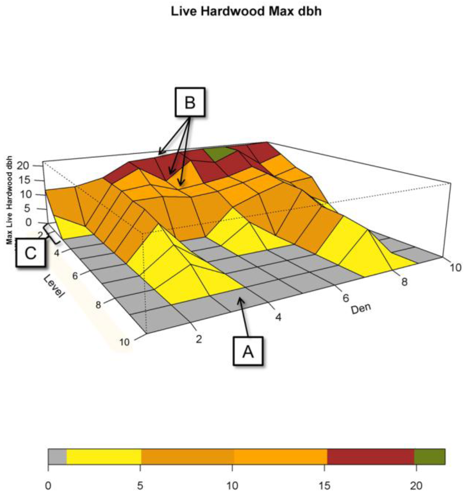
Figure 2 presents a sample of 10 NCs, where each NC is a cluster of 10 neighboring plots (k = 10). Each of these NCs contains a den site. The “Level” axis represents the sorted levels of each of the NCs where l = 1 is the highest valued attribute plot (the “best”) and l = 10 is the lowest valued attribute plot (the “worst”) within an NC. The Den axis represents these 10 NCs, where we have arranged NCs starting with the lowest l = 1 attribute to the den NC with the highest l = 1 attribute. The z-axis (Max Live Hardwood dbh) represents the measured attribute (in this case the dbh of the largest live hardwood found in each level in a given NC). The “topography” in the figure represents the performance of each of the ranked 10 plots associated with respect to this measured attribute. Each facet of the topography represents a given plot and is colored based upon the size of the largest live hardwood found within the plot. In Figure 2, “A” points to a gray colored plot, which indicates that the lowest scoring plot in the fourth NC of this set did not have a live hardwood. “B” represents the maximum values in live hardwood dbh for den NC five at the best (l = 1), second best (l = 2), and third best (l = 3) plots. “C” indicates the region for which most of the largest measured attribute values may be found (l = 1, 2, 3).
Assessment of whether a landscape feature is selective by a fisher takes the form of a test of statistical significance. For a specific landscape measure (e.g., dbh), the test can be used to evaluate whether the distribution of l-th best values in the set of NCs (of k plots each) for a morphological feature (e.g., den sites) is different from the distribution of l-th best values in the set of NCs that do not share that morphological feature (e.g., forest outside home ranges). Evaluation of each l-th ranked landscape measure requires a pairwise test of difference in distribution. The specific approach implemented here, and described fully in Niblett et al. [10] for a simpler form of k-Max-l, uses a non-parametric permutation-based test with the Komolgorov-Smirnov measure of distributional difference. We report p-values for each test based on 9999 permutations and consider results with p-value < 0.05 to be statistically significant. Because there is relatively little overlap between NCs, we did not employ the Bonferroni method [27].
3. Results
Our results presented here are based upon comparing the distribution of l-th ranked plots (for some attribute) within NCs of some spatial extent (for example NCs containing dens) to a distribution of l-th ranked plots of NCs of a different spatial extent (for example forest NCs excluding all den NCs). Table 2 lists the p-values for each attribute listed in Table 1 when comparing NCs containing dens to NCs in the rest of the forest. For many of the attributes, the highest ranked attribute within den NCs was better than what occurred in forest NCs with a p-value of 0.05. Several of the attributes were significant from the best plot attributes (l = 1) through the fifth best (l = 5) for the compared NC distributions. After the l = 6 level, significance of many of the tested attributes were not reported because there was insufficient data to make a valid comparison. This is mainly due to the fact that the comparison distributions have very few attribute features present to compare. In most cases where significance was not reported, far fewer than 50% of the NCs had a measured attribute present. Table 3 presents a comparison between NCs within kernels of female fisher territories vs. NCs of the forest outside all kernels. Table 4 presents a similar comparison, except as applied to den NCs vs. kernel NCs (excluding den NCs). The following three subsections further break down the results presented in these three tables.
3.1. Dens vs. Forest (Table 2)
Most our tests of habitat attributes between Den NCs and Forest NCs excluding dens were significantly different (p ≤ 0.05). The most notable exceptions to significance occur when the level equals or exceeds 3 (l ≥ 3). Attributes that were not significant at some point in this range include: QUADMEAN, BASAL_HW8, TREES_HW, TREES_HW8, and CANOPY. CONIFER_LIVE was not significant where l ≥ 5. Figure 3 depicts three views of the 46 den NCs. The NCs in the top two panels have been sorted based upon the maximum size of the largest live hardwood (dbh in inches) found among the best of the k-plots (where l = 1). They are arranged from left to right (smallest to largest live hardwood tree size for level 1) on the x-axis, or Den axis, in all three panels of the figure. The top panel shows that some den NCs contained few plots with live hardwoods and that in some the largest size was relatively small (25.4 cm, 10 inches dbh). Note the den NCs with the largest live hardwood was approximately 127 cm (50 inches) dbh. The middle plot shows the same ordering of den NCs, but depicts the plots of each NC ordered in terms of the largest live conifer (dbh in inches) found. Note in the case where a large hardwood is not present, a large conifer appears to be present. The bottom panel shows the Den NCs ordered in terms of the size of the maximum live confer (at dbh) found (l = 1). For each NC, the plots are ordered from l = 1 to l = k based upon their rank as to the largest conifer found. It is important to observe here that for many plots associated with den NCs, trees were often not present at levels 8, 9, and 10 and the largest trees, those greater than 50.8 cm (20 inches) were confined principally in the top three levels (l = 1, 2, 3).
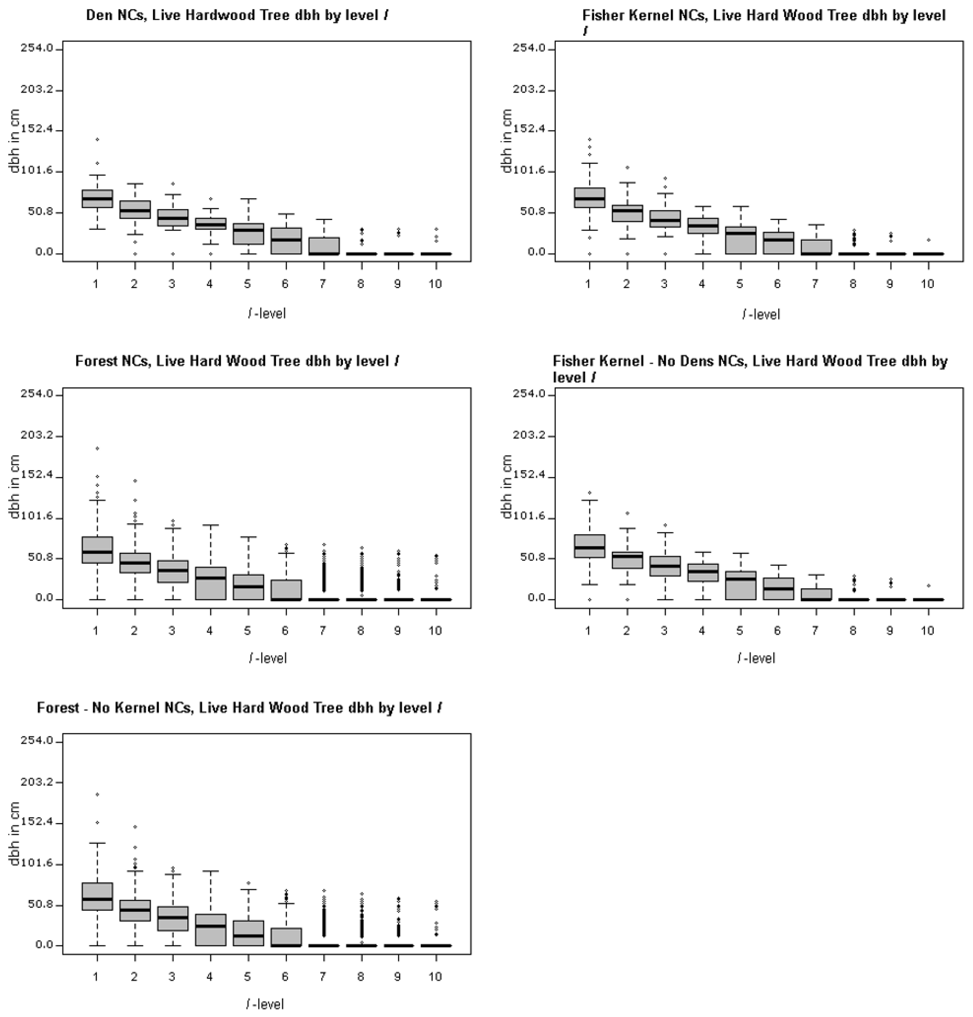
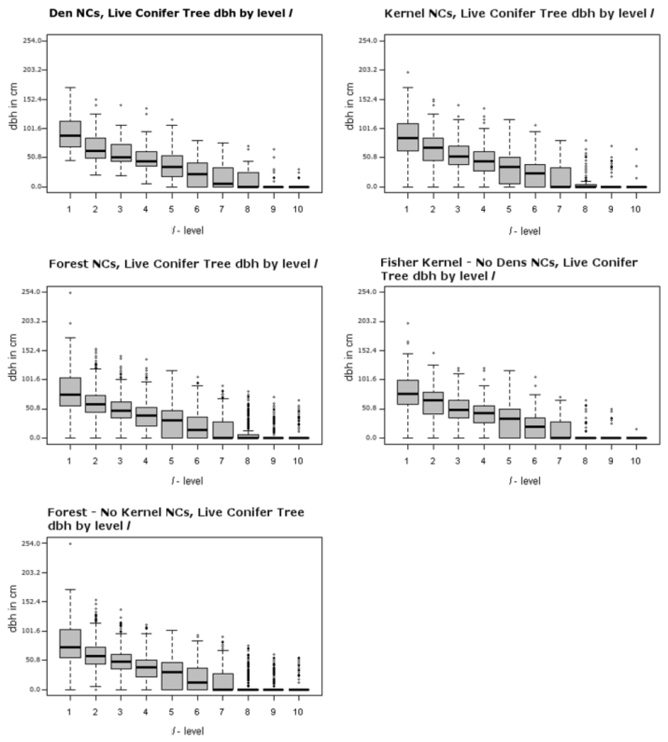
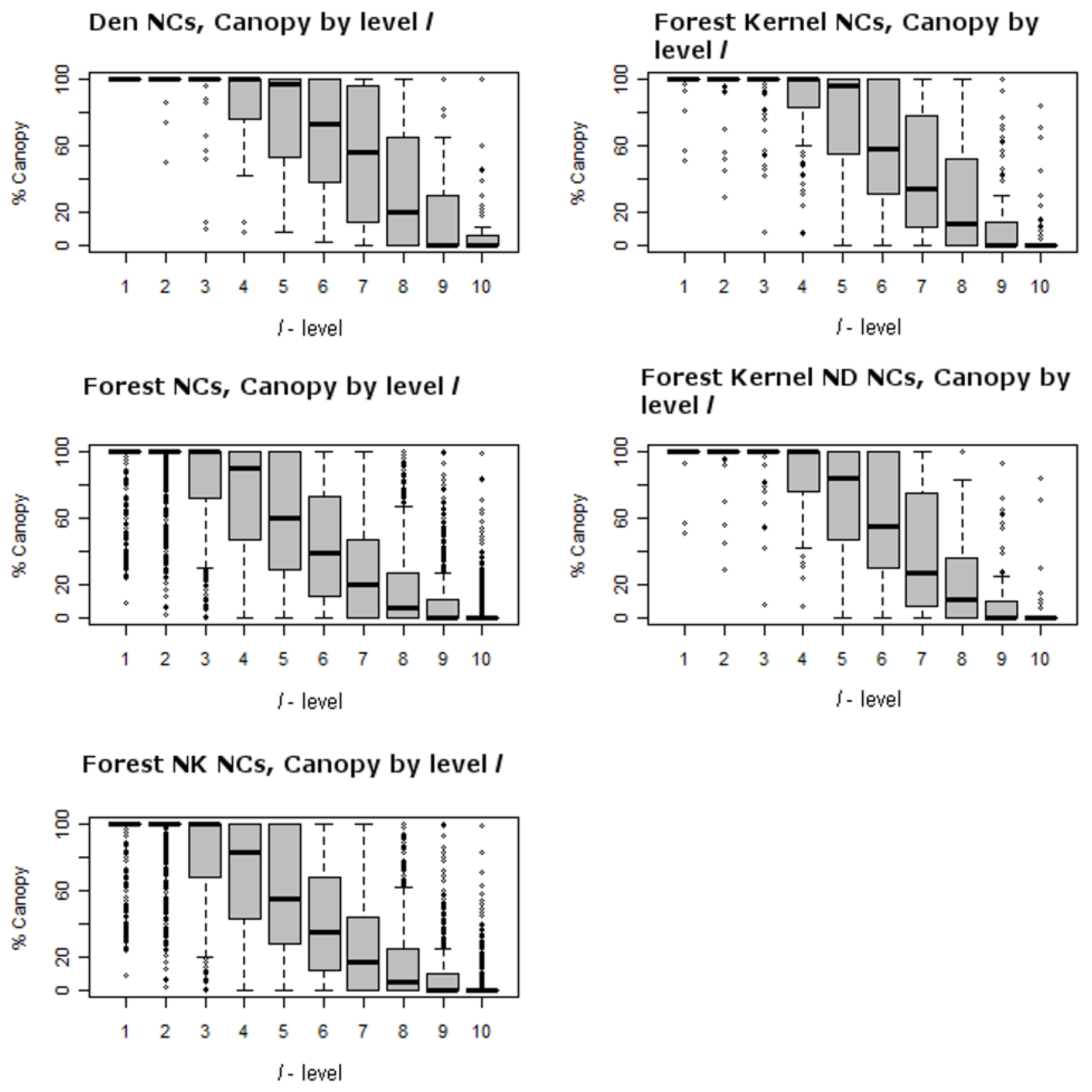
Figure 4 and Figure 5 illustrate the ranges of the largest trees (maximum dbh in cm) found for live hardwoods and conifers across different segments of the forest. There are 5 panels in each of these two figures, including one for den NCs, one for kernel NCs, one for forest NCs, one for kernels excluding den NCs, and one for forest NCs outside kernels. Figure 4 illustrates the largest dbh (in cm) hardwood tree in plot level l for each NC distribution. For example, the top left panel of Figure 4 presents the range of the largest live hardwood trees found across the den NCs. There is a box-whisker plot for each ranking of plots with the den NCs. Similarly, Figure 5 represents the distributions associated with the largest live conifer found based upon plot rankings within NCs. Figure 6 illustrates the Canopy Cover distributions in the same format as Figure 4 and Figure 5. These figures illustrate the presence of the many small openings proximal to den sites, but also across the forest as a whole. For example, the plots ranked as 8 or 9 often contain no sizable or even measurable live conifers or hardwoods for den NCs, kernel NCs, and forest NCs. This means that 8 acres of most 40 acre NCs are either open or have shrubs. Note the median percent canopy is zero for the lowest two ranked plots in NCs, even including den NCs. For example, Table 5 lists the averages for each attribute of each spatial comparison for the ten l level rankings. The den and kernel NC distributions all have higher average attribute measures at all l levels than the remaining forest NC distributions, which is supported by significant selection towards attributes with greater measures (Table 5). The RRHS score was found to be significant at all but the best level (l = 1) for den NCs compared to kernel NCs excluding dens. Unfortunately this specific result is somewhat misleading and this is discussed further in the discussion section.
3.2. Home Range vs. Remaining Forest
Significance testing (Table 3) suggests that the largest measured conifer tree is not a significant component of fisher habitat beyond the fourth level. All of the other measured attributes suggest that these habitat measures are significant. The top right panels of Figure 4, Figure 5 and Figure 6 show the home range (75% KDE) NC distributions over the 10 levels for largest living (dbh) hardwood and conifer, as well as canopy coverage. These panels show that there are similar levels of canopy cover and tree sizes as found in den NC distributions, though often in lower amounts than those measured for den NCs. Table 5 shows this difference in the averages of the NCs representing the various spatial extents. In general, den NCs contain greater amounts of measured attributes than home range NCs than forest NCs (e.g., den NCs > home-range NCs > forest NCs).
3.3. Dens vs Remaining Home Range
All tests comparing den NCs to remaining home range NCs (Table 4) were not significant at the l = 1 level, with the exception of the BIOMASS_AG attribute. At the l = 2 level, TREES_HW, TREES_HW8, and CANOPY were not significant attributes as well. The CONIFER_LIVE attribute was not significant where l ≥ 5. Measured attributes from the den NCs are in general greater in value than home range NCs excluding the dens (Table 5).
4. Discussion
We must first acknowledge that our study area contains a relatively small number of fishers, having only five females tracked over a two-year time span, although our data set contains almost two times the number of den sites as the recent study of Zhao et al. [17]. However, measured den locations and tree sizes in our study area are similar to tree sizes reported in other fisher studies. The results have clearly shown that highly detailed plot data in conjunction with radio-telemetry and other observational data can be used to better understand habitat composition. In this case, habitat that would generally be considered poor using existing models can be shown to contain important distributional compositions using the k-Max-l technique. By utilizing a common analysis unit, the Neighborhood Cluster (NC), a more complete picture emerges with regard to forest habitat use. This technique demonstrates that there is a significant selection by females for those NCs that contain at least a few plots with large trees, even when the landscape is not a continuous canopy covered mature to late seral forest. The fact that most NCs contain at least 2 plots that have few trees suggest that numerous open areas exist even within the neighborhoods chosen by females for denning. Zhao et al. [17] concluded that, “denning structures were associated with forested areas with relatively high canopy cover, large trees, and high levels of vertical structural diversity.” Although it is true that a den site is often surrounded by large trees (based upon a special inventory conducted around each den tree) and perhaps vertical structural diversity, such den sites may not be surrounded by forested stands of high canopy closure within the context of the broader forest area. This is something that Zhao et al. [17] did not address, and that this paper does—how to evaluate a broader area with regard to identifying significant habitat within the broad landscape.
The results help to support the notion that an infrequent inventory plot sampling (e.g., FIA plots of 1 per 2428 ha (6000 acres)) may not be sufficient in estimating or describing habitat suitability for a species like the fisher. It also supports the view that particular features within a matrix of general habitat can be more important, even when not spatially extensive. Within the context of the fisher, those portions of the forest that are older and contain larger trees are indeed significant components of fisher habitat, particularly for den use. Such structures are clearly important for their survival, in that they require such structures for reproduction. However, it is important to understand that large structures are simply not present over great spatial extents and that forest areas consisting of smaller trees with greater canopy openings often occur outside of the best three plots (l > 3) within most NCs. More importantly, it appears that many habitat components are only present in the top 6 levels, leaving the bottom 4 levels to be less than desirable (equivalent to an average of 6.475 ha (16 acres) out of 16.187 ha (40 acres)). This is an important finding, when attempting to define habitat suitability for the fisher. However, the spatial connectivity and clustering of these elements that are core elements of fisher habitat should be further studied. There are several points that need to be further addressed in this discussion.
First, it is important to address a short-coming of the approach related to significance testing with regard to computing the Zielinski RRHS [14] score using plot data attributes. While the Zielinski RRHS score was found to be statistically significant at many levels, the significance may be somewhat misleading in levels that exceed 3 or 4. This is because at such levels the values of the measured attributes are often low, resulting in a low Zielinski score (a score that depicts something that may be avoided). Statistical significance at these levels can also be found when plots with low values of attributes are compared to plots with very low values of attributes, even when one would characterize all such plots as not supportive of the needs of the fisher with respect to dens and resting habitat. That is, comparing poor to very poor is not very informative. While the scores may be subtly different, it is still considered to be poor resting habitat. This suggests that an overall composite score of resting habitat may be less meaningful than considering the attributes themselves. Therefore, while these results are significant as computed using our significance test, they are not meaningful within the context of overall forest composition beyond levels 3 or 4. The major take-away from this is that on the average, stands and cover tend to be low for nearly half the landscape, even for areas close to den and resting sites.
Second, it is important to discuss the findings here with regard to other studies of the fisher, and highlight some of the important implications of this methodology applied at three important scales: comparison of den neighborhoods to a reference potential den neighborhood (den NCs compared to remaining forest NCs), home range components to other remaining potential home range components (home range NCs compared to remaining forest NCs), and how areas surrounding den sites differ from surrounding home range areas (den NCs compared to remaining home range NCs). As one might expect, several attributes of den NCs were significant as compared to NCs in the rest of the forest (Table 2). Many of the attributes related to tree size such as maximum dbh of the largest conifer and the largest hardwood tree, basal area, and tree volume are significant measured at the ranked plot level, l. Notable exceptions that were not significant at the l = 1 level are quadratic mean diameter and the number of hardwood trees greater than or equal to 20.32 cm (8 inches). This indicates that the size distribution of trees, as measured by quadratic mean diameter, is the same as that which is distributed within the forest at the best level (l = 1) in general. However, if one is looking at the largest trees found in den NCs, they are significantly different than what you would find in an average forest NC. That is, the larger hardwood and conifer trees within the forest are generally found in den NCs. Figure 4, Figure 5 and Figure 6 show the ranges for which attribute values occur by level for each of the test and reference distributions. One can think of each of the panels contained within them as being a collapsed version of Figure 3 that shows the overall distribution by level. Figure 4 and Figure 5, top left panels, show that the distribution of large hardwood and conifer structure trees, those with larger dbh, within den NCs is much higher than the remaining forest NCs. For the den NCs where l ≤ 3 (the best three plots), the average size of the largest conifers found is 76.5 cm (30.1 inches) dbh in size. The average largest conifer dbh over the range of significance in den NCs (levels 1:4) is 70.2 cm (27.6 in). Similarly, the largest hardwood found in den NCs where l ≤ 3 average dbh is 55.9 cm (22.0 in), and 40.8 cm (16.1 in) over the range of significance (levels 1 through 6). Typically, the best plot (l = 1) had a conifer at least 76.2 cm (30.0 inches) or a hardwood that was at least 50.8 cm (20.0 inches). These were in line with the measured attributes of known den trees (Table 6). The average black oak hardwood den tree, the tree used for a majority of den sites, was 53.3 cm (21.0 inches). In general, black oaks used for denning appear to have lower average dbh (53.3 cm, 21.0 inches) than other hardwood species dbh used for denning which average 65.2 cm (25.7 inches). Both of these averages, black oak and other hardwood den trees, are less than the average resting hardwood dbh (69.0 cm, 27.17 inches) reported by Zielinski et al. [20] for California fisher in northern California coastal and Sierra Nevada ranges.
Dens in live conifer trees, in this case Douglas fir, were in larger trees where average dbh was 129.79 cm (51.10 inches), though there was a total of just three dens in this type of tree (they measured 189.99, 134.11, and 65.28 cm (74.80, 52.80, and 25.70 inches)). Thus, the confidence in the average size of a potentially suitable Douglas fir den tree is not high as there is great variability in tree size. Nevertheless, the average dbh size of living Douglas fir (129.79 cm, 51.10 inches) and snag (119.43 cm, 47.02 inches) den trees are similar in size to resting live conifer (117.3 cm, 46.18 inches) and snag (119.8 cm, 47.17 inches) trees described by Zielinski et al. [20]. The den conifers size found in this study are also larger than the average dbh for live conifer (97.40 cm, 38.35 inches) and snag (98.83 cm, 38.91 inches) resting trees described by Purcell et al. [28] for a Sierra Nevada fisher population. This is similar to the average dbh of the largest living conifer tree found at the best level (l = 1) in the den NCs of our study area (94.26 cm, 37.11 inches). Zhao et al. [17] used LiDAR data in a Sierra Nevada forest to determine forest structure tree size and density about fisher den sites for 20, 30, and 50 m. ranges. They found that den structure trees in their study area tended to be clustered with other large trees within circles of those radii. Our result appears to confirm this, albeit in a forest with greater fragmentation. Given that the top 3 l-levels contain a large live conifer tree (>50.8 cm, 20 inches), a greater proportion of total basal area, and Scribner volume which are indicative of the presence of other large trees, it is likely that there are other large structures near the largest measured tree.
Figure 4 and Figure 5, top left panel, illustrate the range of largest dbh of live hardwood and conifer trees for dens over the l-levels. The middle left panels of Figure 4 and Figure 5 illustrate the range for the forest NCs excluding dens over the l-levels. They clearly illustrate that the largest trees are generally concentrated in the best ranked plots; tree size drops off dramatically as one moves toward lower ranked l levels starting around the 4th and 5th levels. In addition to the larger trees, there appears to be greater amounts of measured above ground biomass in average den NCs as compared to average forest NCs (Table 5). The average above ground biomass difference between the top three levels (l ≥ 3) of den NCs to forest NCs exceeds 100 metric tons per hectare; for mid-levels (l = 4, …, 8) it is between 100 and 50 metric tons per hectare; and for the lower levels (l = 9 and 10) it is less than 50 tons per hectare. This suggests that den NCs generally contain greater portions of forest than an average forest NC where above ground biomass is generally much less. It is no surprise then that canopy cover is significant for fisher home ranges, but for l = 4, …, 8, there is likely to be a greater portion of forest openings. Significance of canopy is found when comparing den NCs to home range NCs at levels 3–8. This suggests that canopy cover for den NCs is greater than that of home range NCs. This is also confirmed by the higher levels of canopy cover generally found for den and home range NCs as compared to the general forest found in Table 5.
Third, it is important to understand how this forest differs from that of other studies that suggest that extensive moderate to dense canopy cover is an important predictor of fisher habitat and where fisher home ranges consisted of less than 5% forest openings (e.g., [22]). Level of canopy cover has been termed dense (100–60%), moderate (59–40%), open (39–25%), and sparse (<25%) using the California Wildlife Habitat Relationship (CWHR) system by Mayer and Laudenslayer [29]. Our study area contains a much greater proportion of forest area that is open, 24% of the study area, than what has been suggested as essential. For example, total canopy closure within den NCs drops below 40% after the l = 6 level (Table 5). Figure 6 (top left panel) shows the canopy cover distributions for ranked plots (l-level) within NCs as box-whisker plots. For l = 1 to 5, canopy is dense. In l = 6 and 7 canopy cover is moderate and for l = 8, 9, and 10 it is open to sparse. It is clear that for other NC comparisons where l = 8, 9, and 10, a majority of the NCs contain sparse to open canopy cover as well. This suggests that fisher indeed requires dense canopy for portions of their home range and den sites. This is similar to what Zhao [17] observed. Heterogeneous forests are also likely to contain greater numbers of hardwoods, which appear to be critical den structures—they were the greatest types of structures used for denning in this study area, and how den cavities form [30].
Finally, it should be underscored here that a suitable unit of analysis and methodology for understanding portions of that unit must be used when attempting to understand broad scale habitat requirements for a species. This is especially true within the context of developing rules for environmental planning and analysis. We also believe that the framework of this paper may be used to evaluate other species habitat requirements to make informed policy based upon best science.
5. Conclusions
This research has significant implications for management strategies for the future provision and current protection of habitat, especially fisher habitat. This is a first attempt at addressing the spatial extent to which habitat must be an older, mature forest, generally accepted as a major habitat requirement. To address this question, we developed a framework called k-Max-l. Using this approach we are able to determine significant habitat components even when they are not spatially abundant. One key finding is that fishers occupied neighborhood clusters that often contained open areas of up to 25%, and their den sites often involved one of the largest available trees in the cluster, even when such sites were scarce and close to plots that were classified as open. This new k-Max-l approach can help to identify and understand the distribution of critical habitat elements as well as help in developing metrics for analyzing and managing habitat over time. It is necessary that long-term spatially extensive management considerations account for these types of habitat complexities in order to ensure long term fisher occupation.
In this study, we have analyzed an area where significant portions of the forest contain few large trees and where there are numerous openings in significantly greater proportions than previously reported in the literature [22] as being needed for fisher habitat. However, we have also shown that the few large trees that do exist, particularly those in areas where their numbers are higher, tend to be near den locations and within home ranges. This appears to agree with the recent work of Zhao et al. [17] which involved LiDAR to determine the density of other large trees in close proximity to known den sites in an area inhabited by the fisher. Our approach is the first such study that has used detailed fine scale plot data collected over a large forested area. Because of this, we could group this fine scale data into larger, meaningful spatial units, called Neighborhood Clusters or NCs. Neighborhood Clusters could then be classified as to whether they contain a Den site, are part of known habitat as defined by kernel density estimates of female fisher territories, or part of the remaining landscape. Distributions of habitat elements within each neighborhood cluster can then be compared to test significance even when larger average forest measures lack explanatory power.
There are three elements not addressed in this study but which are of great concern. The first is that there is an assumption that a large tree contains a suitable cavity. While this is likely to be true for our study area given its prior land use, if forest conditions change due to increased logging activity and management, caution should be used when using this measure. The reason for this concern is as follows. Though large trees, either at or exceeding the size of current ones, can be produced faster in an industrial forest it is unknown if a cavity potentially useful to denning will be produced in that same length of time as in less managed areas. It seems clear that maintaining suitable conditions for the fisher, when an area may be subject to logging, will require a significant effort to maintain older and larger trees, even in areas being cut, to ensure that regenerated stands exist over time that have a number of suitable structures, canopy, and that the density of such stands is high enough to support movement between suitable “denning site” neighborhood clusters. These constraints may be significant in controlling the spatial arrangements in harvesting while maintaining a landscape suitable for the fisher, as well as potentially extend rotation schedules significantly beyond 100 or more years. Thus, attention should be focused on understanding how to use data such as this to evaluate plans that alter the landscape, such as logging activities, in order to maintain and provide future conditions suitable for species habitat.
The second element is that existing hardwoods present in the forest have played an important role in supporting the fisher, as they have provided many suitable denning sites. If the area is managed so that hardwoods are eliminated in the regeneration process with a move to replant only conifers, larger and older conifers will be necessary to support this function over time.
The third is that while the k-Max-l method shows that the proportion of large trees suitable for resting and denning are not spatially extensive, and are likely clustered, there is no information related to connectivity. This is an important area of future research that should be explored as this is likely to provide greater insight into how a home range is connected, and thus supportive of the fisher. Such an understanding would aid in estimating the impacts of proposed management activities on possible habitat. Understanding this third point is of great importance as a majority of a fisher home range appears to be connected in some way with canopy cover and the presence of suitable den and rest trees. Even though there are numerous openings surrounded by forest stands of varying age, we have assumed here that there is a matrix of forest stands that are reasonably connected. An initial analysis of this tends to bear this out. We suspect that isolated NCs, regardless of their quality, should not be considered viable for denning or as part of a possible home-range.
Future work will help to further characterize the needs of the fisher, but several elements have been uncovered in this work that have significant management implications. We found that fishers select areas of denser forest with large trees for den site areas, and that to maintain fisher populations on their lands, and reduce adverse impacts, private timberland owners may wish to take this into account when planning logging activities.
Acknowledgments
We wish to acknowledge a generous gift from the California Forestry Association that helped support this research. We also would like to thank Sierra Pacific Industries for providing inventory data and also want to acknowledge the use of traps, tracking, and den site data collected under the supervision of the California Department of Fish and Wildlife.
Author Contributions
M.R.N., S.H.S., and R.L.C. conceived and designed the methodology used in this paper. K.H.B. provided technical consultation. M.R.N. and S.H.S. analyzed the data. M.R.N. wrote the initial draft of the paper, and R.L.C., S.H.S., and K.H.B. helped edit it.
Conflicts of Interest
The authors declare no conflict of interest. The funding sponsors had no role in the design of the study; in the analyses, or interpretation of data; in the writing of the manuscript, and in the decision to publish the results.
References
- Gerrard, R.; Stine, P.; Church, R.; Gilpin, M. Habitat evaluation using GIS: A case study applied to the San Joaquin Kit Fox. Landsc. Urban Plan. 2001, 52, 239–255. [Google Scholar] [CrossRef]
- Koopman, M.E.; Scrivner, J.H.; Kato, T.T. Patterns of den use by San Joaquin kit foxes. J. Wildl. Manag. 1998, 62, 373–379. [Google Scholar] [CrossRef]
- Morrell, S.H. The Life History of the San Joaquin Kit Fox. Master’s Thesis, Department of Zoology, University of California, Santa Barbara, CA, USA, 1971. [Google Scholar]
- Ralls, K.; White, P.J. Predation on San Joaquin kit foxes by larger canids. J. Mammal. 1995, 76, 723–729. [Google Scholar] [CrossRef]
- White, P.J.; Ralls, K. Reproduction and spacing patterns of kit foxes relative to changing prey availability. J. Wildl. Manag. 1993, 57, 861–867. [Google Scholar] [CrossRef]
- Bjurlin, C.D.; Cypher, B.L.; Wingert, C.M.; Van Horn Job, C.L. Urban Roads and the Endangered San Joaquin Kit Fox; Final Report Submitted to the California Department of Transportation by the California State University, Stanislaus Endangered Species Recovery Program; California Department of Transportation: Sacramento, CA, USA, 2005; pp. 1–47.
- Chawkins, S. Kit Foxes Make Themselves at Home within Bakersfield City Limits; Los Angeles Times: Los Angeles, CA, USA, 2012. [Google Scholar]
- Sato, J.J.; Mieczyslaw, W.; Prevosti, F.J.; D'Elía, G.; Begg, C.; Begg, K.; Hosoda, T.; Campbell, K.; Suzuki, H. Evolutionary and biogeographic history of weasel-like carnivorans (Musteloidea). Mol. Phylogenet. Evol. 2012, 63, 745–757. [Google Scholar] [CrossRef] [PubMed]
- Zielinski, W.J.; Truex, R.L.; Schmidt, G.A.; Schlexer, F.V.; Schmidt, K.N.; Barrett, R.H. Home range characteristics of fishers in California. J. Mammal. 2004, 85, 649–657. [Google Scholar] [CrossRef]
- Niblett, M.R.; Sweeney, S.H.; Church, R.L.; Barber, K.H. Structure of fisher (Pekania pennanti) habitat in a managed forest in an interior northern California coast range. For. Sci. 2015, 61, 481–493. [Google Scholar] [CrossRef]
- Sweitzer, R.A.; Furnas, B.J.; Barrett, R.H.; Purcell, K.L.; Thompson, C.M. Landscape fuel reduction, forest fire, and biophysical linkages to local habitat use and local persistence of fishers (Pekania pennanti) in Sierra Nevada mixed-conifer forests. For. Ecol. Manag. 2016, 361, 208–225. [Google Scholar] [CrossRef]
- Buck, S.G.; Mullis, C.; Mossman, A.S.; Show, I.; Coolahan, C. Habitat use by fishers in adjoining heavily and lightly harvested forest. In Martens, Sables, and Fishers: Biology and Conservation; Buskirk, S.W., Harestad, A.S., Raphael, M.G., Powell, R.A, Eds.; Cornell University Press: Ithaca, NY, USA, 1994; pp. 368–376. [Google Scholar]
- The United States Department of Agriculture (USDA). Forest Inventory and Analysis National Program. 2013. Available online: http://www.fia.fs.fed.us/library/fact-sheets/data-collections/Phase2_3 (accessed on 11 February 2017).
- Zielinski, W.J.; Dunk, J.R.; Gray, A.N. Estimating habitat value using forest inventory data: The fisher (Martes pennanti) in northwestern California. For. Ecol. Manag. 2012, 275, 35–42. [Google Scholar] [CrossRef]
- Reno, M.A.; Rulon, K.R.; James, C.E. Fisher Monitoring within Two Industrially Managed Forests of Northern California: Progress Report to the California Department of Fish and Game; Sierra Pacific Industries: Anderson, CA, USA, 2008. [Google Scholar]
- Lofroth, E.C.; Raley, C.M.; Higley, J.M.; Truex, R.L.; Yaeger, J.S.; Lewis, J.C.; Happe, P.J.; Finley, L.L.; Naney, R.H.; Hale, L.J.; et al. Conservation of Fishers (Martes pennanti) in South-Central British Columbia, Western Washington, Western Oregon, and California; Volume I: Conservation Assessment; Bureau of Land Management, United States Department of the Interior: Denver, CO, USA, 2010.
- Zhao, F.; Sweitzer, R.; Guo, Q.; Kelly, M. Characterizing habitats associated with fisher den structures in the Southern Sierra Nevada, California using discrete return LiDAR. For. Ecol. Manag. 2012, 280, 112–119. [Google Scholar] [CrossRef]
- Diggle, P.J. A kernel method for smoothing point process data. Appl. Stat. 1985, 34, 138–147. [Google Scholar] [CrossRef]
- Diggle, P.J. Statistical Analysis of Spatial Point Patterns, 2nd ed.; Hodder Education Publishers: London, UK, 2003. [Google Scholar]
- Zielinski, W.J.; Truex, R.L.; Schmidt, G.A.; Schlexer, F.V.; Schmidt, K.N.; Barrett, R.H. Resting habitat selection by fishers in California. J. Wildl. Manag. 2004, 68, 475–492. [Google Scholar] [CrossRef]
- Aubry, K.B.; Raley, C.M.; Buskirk, S.W.; Zielinski, W.J.; Schwartz, M.K.; Golightly, R.T.; Purcell, K.L.; Weir, R.D.; Yaeger, J.S. Meta-analyses of habitat selection by fishers at resting sites in the Pacific Coastal Region. J. Wildl. Manag. 2013, 77, 965–974. [Google Scholar] [CrossRef]
- Raley, C.M.; Lofroth, E.C.; Truex, R.L.; Yaeger, J.S.; Higley, J.M. Habitat ecology of fishers in western north America. In Biology and Conservation of Martens, Sables, and Fishers: A New Synthesis; Aubry, K.B., Zielinski, W.J., Raphael, M.G., Proulx, G., Buskirk, S.W., Eds.; Cornell University Press: Ithaca, NY, USA, 2012; pp. 231–254. [Google Scholar]
- Davis, F.W.; Seo, C.; Zielinski, W.J. Regional variation in home-range-scale habitat models for fisher (Martes pennanti) in California. Ecol. Appl. 2007, 17, 2195–2213. [Google Scholar] [CrossRef] [PubMed]
- Matthews, S.M.; Higley, J.M.; Rennie, K.M.; Green, R.E.; Goddard, C.A.; Wengert, G.M.; Gabriel, M.W.; Fuller, T.K. Reproduction, recruitment, and dispersal of fishers (Martes pennanti) in a managed Douglas-fir forest in California. J. Mammal. 2013, 94, 100–108. [Google Scholar] [CrossRef]
- Sweitzer, R.A.; Popescu, V.D.; Barrett, R.H.; Purcell, K.L.; Thompson, C.M. Reproduction, abundance, and population growth for a fisher (Pekania pennanti) population in the Sierra National Forest, California. J. Mammal. 2015, 96, 772–790. [Google Scholar] [CrossRef]
- McCann, N.P.; Zollner, P.A.; Gilbert, J.H. Bias in the use of broadscale vegetation data in the analysis of habitat selection. J. Mammal. 2014, 95, 369–381. [Google Scholar] [CrossRef]
- Cabin, R.J.; Mitchell, R.J. To Bonferroni or not to Bonferroni: When and how are the questions. Bull. Ecol. Soc. Am. 2000, 81, 246–248. [Google Scholar]
- Purcell, K.L.; Mazzoni, A.K.; Mori, S.R.; Boroski, B.B. Resting structures and resting habitat of fishers in the southern Sierra Nevada, California. For. Ecol. Manag. 2009, 258, 2696–2706. [Google Scholar] [CrossRef]
- Mayer, K.E.; Laudenslayer, W.F. A Guide to Wildlife Habitats of California; California Department of Fish and Game: Sacramento, CA, USA, 1988.
- Weir, R.D.; Phinney, M.; Lofroth, E.C. Big, sick, and rotting: Why tree size, damage, and decay are important to fisher reproductive habitat. For. Ecol. Manag. 2012, 265, 230–240. [Google Scholar] [CrossRef]
Figure 1.
Forest study area in Trinity County, California, CA, USA.
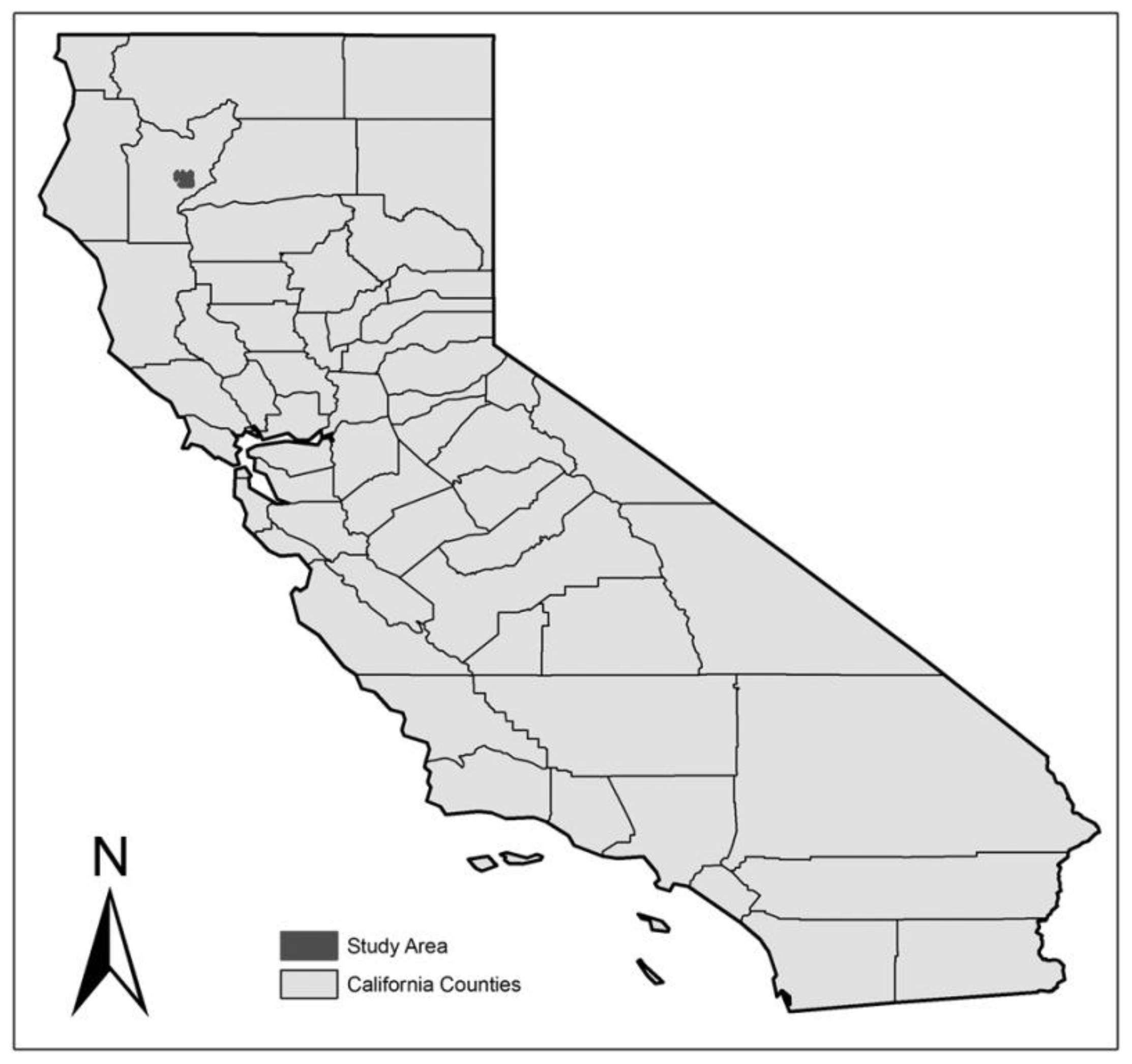
Figure 2.
Example of NCs of size k = 10 plots (10-Max) that contain den sites where plots within each NC are ranked from l = 1 to 10. The Den axis represents 10 such den NCs. The Level axis represents the ranked plots within each NC from best (1) to worst (10). (A) shows the lowest ranked areas that have low attribute measures; The “topography” (B) represents the size of Maximum Live Hardwood, dbh, found across plots within each NC. The color scale represents the size of the largest live hardwood in a given plot based upon the diameter at breast height (measured in inches); (C) shows the top 3 ranks.

Figure 3.
Sorted Den NCs for Live Hardwood Maximum dbh and Live Conifer Maximum dbh, in inches. The top panel shows the Live Hardwood Maximum dbh sorted by Den from low to high for the highest ranked plot in each NC (that is, l = 1). The middle panel shows Live Conifer Maximum dbh using the same Den sorting from the top panel. The bottom panel shows the den NCs sorted by the highest ranked plot in each NC in terms of the largest conifer found.
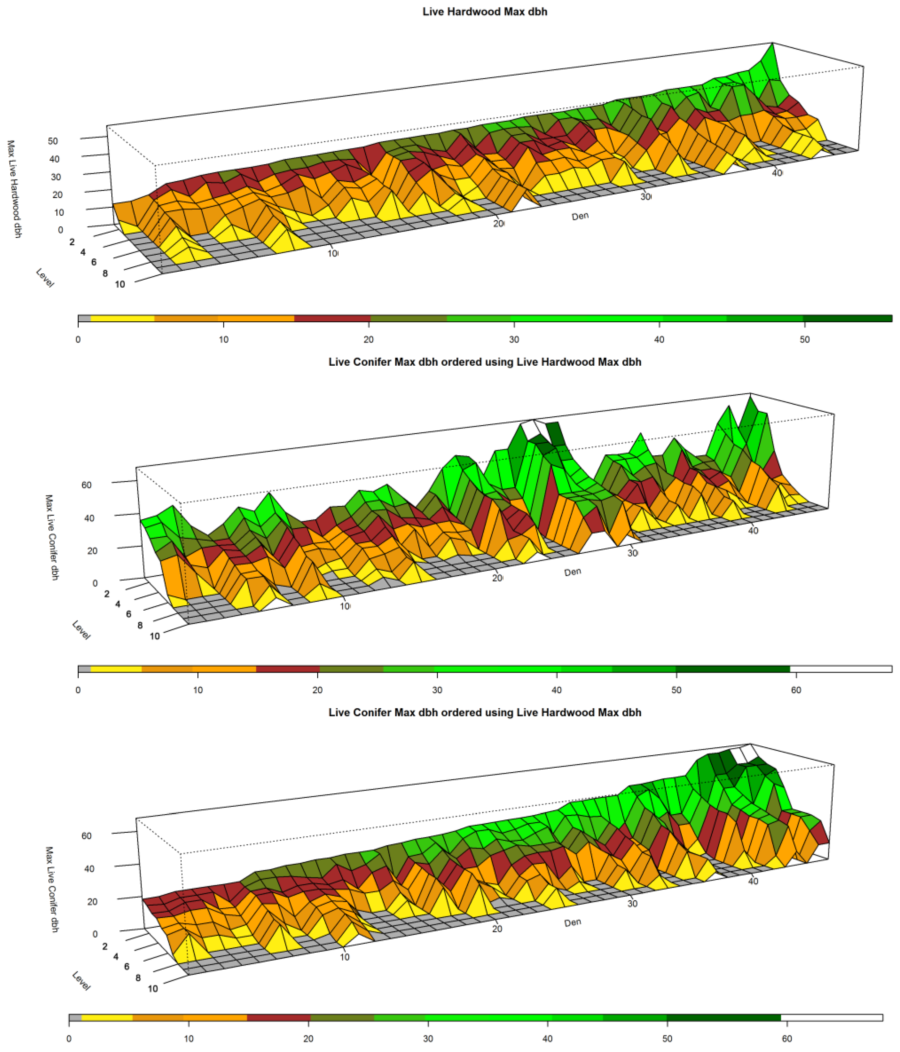
Figure 4.
Largest dbh hardwood tree in plot level l for each NC distribution from left to right: Den, Kernel, Forest, Kernel excluding den NCs, and Forest excluding kernel NCs. Solid bar represents the median, gray box represents the 25% quartile above and below the mean, and the whiskers represent 3.5 times the upper and lower values of the gray box. The dots are individual values that lie outside the whiskers.

Figure 5.
Largest dbh conifer tree in plot level l for each quadrature distribution from left to right: Den, Kernel, Forest, Kernel excluding den NCs, and Forest excluding kernel NCs. Solid bar represents the median, gray box represents the 25% quartile above and below the mean, and the whiskers represent 3.5 times the upper and lower values of the gray box. The dots are individual values that lie outside the whiskers.

Figure 6.
Canopy distributions over each k-Max-l level for each spatial distribution set. NC spatial sets are from top left to right: den, kernel, forest, forest excluding den sites, and forest excluding kernel. Solid bar represents the median, gray box represents the 25% quartile above and below the mean, and the whiskers represent 3.5 times the upper and lower values of the gray box. The dots are individual values that lie outside the whiskers.


Table 1.
A selected subset of attributes collected at each plot as well as the Relative Resting Habitat Suitability (RRHS) scores derived from these attributes using the method of Zielinski et al. [14].
Table 1.
A selected subset of attributes collected at each plot as well as the Relative Resting Habitat Suitability (RRHS) scores derived from these attributes using the method of Zielinski et al. [14].
| Attribute | Attribute Code | Measurement Unit |
|---|---|---|
| Quadratic mean dbh | QUADMEAN | cm |
| Douglas fir basal area | BASAL_DF | m2 ha−1 |
| Hardwood basal area | BASAL_HW | m2 ha−1 |
| Hardwood basal area where dbh ≥ 20.32 cm | BASAL_HW8 | m2 ha−1 |
| Snag basal area | BASAL_SNAG | m2 ha−1 |
| Douglas fir Scribner volume | SCRIB_DF | Board-feet per acre |
| Canopy cover | CANOPY | Percent canopy cover (100% = complete cover) |
| Number of Douglas fir trees | TREES_DF | Trees per hectare |
| Number of hardwood trees | TREES_HW | Trees per hectare |
| Number of hardwood trees ≥ 20.32 cm | TREES_HW8 | Trees per hectare |
| Largest dbh conifer tree in plot | CONIFER_LIVE | cm |
| Largest dbh hardwood in plot | HARDWOOD_LIVE | cm |
| Above ground biomass | BIOMASS_AG | Metric tons ha−1 |
| RRHS Score | z_RRHS | Values range from 0 to 1 |
Table 2.
p-Values for attributes at level l for den NCs compared to forest NCs.
| Attribute | Level l | |||||||||
|---|---|---|---|---|---|---|---|---|---|---|
| 1 | 2 | 3 | 4 | 5 | 6 | 7 | 8 | 9 | 10 | |
| QUADMEAN | 0.264 | 0.005 | 0.002 | 0.001 | 0.001 | 0.001 | 0.001 | 0.009 | - | - |
| BASAL_DF | 0.002 | 0.002 | 0.001 | 0.001 | 0.001 | - | - | - | - | - |
| BASAL_HW | 0.004 | 0.050 | 0.023 | 0.001 | 0.001 | 0.001 | - | - | - | - |
| BASAL_HW8 | 0.010 | 0.066 | 0.004 | 0.001 | 0.001 | - | - | - | - | - |
| SCRIB_DF | 0.001 | 0.001 | 0.001 | 0.001 | 0.001 | - | - | - | - | - |
| TREES_DF | 0.002 | 0.001 | 0.001 | 0.001 | 0.002 | - | - | - | - | - |
| TREES_HW | 0.006 | 0.089 | 0.018 | 0.001 | 0.001 | 0.001 | - | - | - | - |
| TREES_HW8 | 0.235 | 0.231 | 0.013 | 0.001 | 0.001 | - | - | - | - | - |
| CANOPY | 0.050 | 0.065 | 0.060 | 0.028 | 0.005 | 0.003 | 0.001 | 0.001 | - | - |
| BASAL_SNAG | 0.001 | - | - | - | - | - | - | - | - | - |
| BIOMASS_AG | 0.001 | 0.001 | 0.001 | 0.001 | 0.001 | 0.001 | 0.001 | 0.001 | - | - |
| z_RRHS | 0.003 | 0.001 | 0.001 | 0.001 | 0.001 | 0.001 | 0.001 | 0.001 | 0.001 | 0.003 |
| CONIFER_LIVE | 0.042 | 0.050 | 0.043 | 0.032 | 0.061 | 0.253 | - | - | - | - |
| HARDWOOD_LIVE | 0.009 | 0.005 | 0.003 | 0.001 | 0.018 | 0.004 | - | - | - | - |
An-indicates insufficient data to determine statistical significance (fewer than 50% of an attribute of the comparison distribution were present).
Table 3.
p-Values for attributes at level l for kernel NCs compared to forest NCs excluding kernels.
Table 3.
p-Values for attributes at level l for kernel NCs compared to forest NCs excluding kernels.
| Attribute | Level l | |||||||||
|---|---|---|---|---|---|---|---|---|---|---|
| 1 | 2 | 3 | 4 | 5 | 6 | 7 | 8 | 9 | 10 | |
| QUADMEAN | 0.001 | 0.001 | 0.001 | 0.001 | 0.001 | 0.001 | 0.002 | 0.003 | - | - |
| BASAL_DF | 0.001 | 0.001 | 0.001 | 0.001 | 0.001 | - | - | - | - | - |
| BASAL_HW | 0.006 | 0.001 | 0.001 | 0.001 | 0.001 | 0.001 | - | - | - | - |
| BASAL_HW8 | 0.007 | 0.001 | 0.001 | 0.001 | 0.001 | - | - | - | - | - |
| SCRIB_DF | 0.001 | 0.001 | 0.001 | 0.001 | 0.001 | - | - | - | - | - |
| TREES_DF | 0.001 | 0.001 | 0.001 | 0.001 | 0.001 | - | - | - | - | - |
| TREES_HW | 0.002 | 0.011 | 0.001 | 0.001 | 0.001 | 0.001 | - | - | - | - |
| TREES_HW8 | 0.009 | 0.001 | 0.001 | 0.001 | 0.001 | - | - | - | - | - |
| CANOPY | 0.047 | 0.001 | 0.001 | 0.001 | 0.001 | 0.001 | 0.001 | 0.006 | - | - |
| BASAL_SNAG | 0.001 | - | - | - | - | - | - | - | - | - |
| BIOMASS_AG | 0.001 | 0.001 | 0.001 | 0.001 | 0.001 | 0.001 | 0.001 | 0.001 | - | - |
| z_RRHS | 0.002 | 0.001 | 0.001 | 0.001 | 0.001 | 0.001 | 0.001 | 0.001 | 0.001 | 0.004 |
| CONIFER_LIVE | 0.050 | 0.002 | 0.020 | 0.009 | 0.060 | 0.211 | - | - | - | - |
| HARDWOOD_LIVE | 0.001 | 0.003 | 0.002 | 0.001 | 0.001 | 0.001 | - | - | - | - |
An-indicates insufficient data to determine statistical significance (fewer than 50% of an attribute of the comparison distribution were present).
Table 4.
p-Values for attributes at level l for den NCs compared to kernel NCs excluding den NCs.
| Attribute | Level l | |||||||||
|---|---|---|---|---|---|---|---|---|---|---|
| 1 | 2 | 3 | 4 | 5 | 6 | 7 | 8 | 9 | 10 | |
| QUADMEAN | 0.548 | 0.002 | 0.001 | 0.001 | 0.001 | 0.001 | 0.001 | 0.001 | - | - |
| BASAL_DF | 0.174 | 0.001 | 0.001 | 0.001 | 0.001 | - | - | - | - | - |
| BASAL_HW | 0.107 | 0.023 | 0.007 | 0.001 | 0.001 | 0.001 | - | - | - | - |
| BASAL_HW8 | 0.164 | 0.016 | 0.002 | 0.001 | 0.001 | - | - | - | - | - |
| SCRIB_DF | 0.119 | 0.001 | 0.001 | 0.001 | 0.001 | - | - | - | - | - |
| TREES_DF | 0.230 | 0.001 | 0.001 | 0.001 | 0.002 | - | - | - | - | - |
| TREES_HW | 0.209 | 0.079 | 0.008 | 0.001 | 0.001 | 0.001 | - | - | - | - |
| TREES_HW8 | 0.985 | 0.102 | 0.003 | 0.001 | 0.001 | - | - | - | - | - |
| CANOPY | 0.169 | 0.059 | 0.021 | 0.008 | 0.001 | 0.001 | 0.001 | 0.003 | - | - |
| BASAL_SNAG | 0.121 | - | - | - | - | - | - | - | - | - |
| BIOMASS_AG | 0.002 | 0.001 | 0.001 | 0.001 | 0.001 | 0.001 | 0.001 | 0.001 | - | - |
| z_RRHS | 0.190 | 0.001 | 0.001 | 0.001 | 0.001 | 0.001 | 0.001 | 0.001 | 0.001 | 0.002 |
| CONIFER_LIVE | 0.446 | 0.023 | 0.026 | 0.037 | 0.056 | 0.209 | - | - | - | - |
| HARDWOOD_LIVE | 0.464 | 0.002 | 0.003 | 0.001 | 0.003 | 0.002 | - | - | - | - |
An-indicates insufficient data to determine statistical significance (fewer than 50% of an attribute of the comparison distribution were present).
Table 5.
Average of attributes over all l levels for each spatial comparison: Den NCs, kernel NCs, kernel NCs excluding dens (Kernels ND), forest excluding kernels (Forest NK), and the forest.
Table 5.
Average of attributes over all l levels for each spatial comparison: Den NCs, kernel NCs, kernel NCs excluding dens (Kernels ND), forest excluding kernels (Forest NK), and the forest.
| Level l | Quadratic Mean Diameter | Douglas Fir Basal Area | ||||||||
|---|---|---|---|---|---|---|---|---|---|---|
| Den | Kernels | Kernels ND | Forest NK | Forest | Den | Kernels | Kernels ND | Forest NK | Forest | |
| 1 | 65.3050 | 68.3211 | 67.7915 | 64.8644 | 65.1384 | 42.22 | 36.64 | 33.83 | 26.91 | 28.15 |
| 2 | 52.1170 | 51.1282 | 50.4853 | 46.9232 | 47.4318 | 28.21 | 23.79 | 20.05 | 15.75 | 16.85 |
| 3 | 45.2104 | 41.6991 | 40.4339 | 38.6240 | 39.0080 | 22.13 | 17.34 | 14.53 | 9.88 | 10.92 |
| 4 | 38.5410 | 35.8297 | 34.8374 | 31.7737 | 32.3168 | 15.79 | 11.99 | 10.21 | 6.39 | 7.16 |
| 5 | 32.9805 | 30.3389 | 29.9172 | 26.6710 | 27.1301 | 10.48 | 8.42 | 7.43 | 4.09 | 4.71 |
| 6 | 27.9789 | 25.8853 | 25.0440 | 21.9296 | 22.4401 | 8.02 | 5.94 | 4.74 | 2.31 | 2.81 |
| 7 | 23.2950 | 20.3291 | 18.6134 | 17.0014 | 17.4266 | 4.95 | 3.71 | 2.68 | 1.14 | 1.50 |
| 8 | 17.2574 | 15.1629 | 13.8147 | 11.6828 | 12.1332 | 2.84 | 2.08 | 1.30 | 0.55 | 0.76 |
| 9 | 10.5334 | 9.2376 | 8.4207 | 7.0595 | 7.3483 | 1.39 | 0.91 | 0.57 | 0.12 | 0.22 |
| 10 | 5.4918 | 3.2463 | 2.6177 | 2.7027 | 2.7979 | 0.78 | 0.32 | 0.13 | 0.05 | 0.09 |
| Average | 31.8711 | 30.1178 | 29.1976 | 26.9232 | 27.3171 | 13.68 | 11.11 | 9.55 | 6.72 | 7.32 |
| Level l | Hardwood basal area | Hardwood ≥ 20.32cm basal area | ||||||||
| Den | Kernels | Kernels ND | Forest NK | Forest | Den | Kernels | Kernels ND | Forest NK | Forest | |
| 1 | 64.70 | 60.31 | 59.00 | 48.40 | 49.95 | 43.44 | 39.60 | 37.85 | 32.50 | 33.47 |
| 2 | 36.87 | 36.85 | 36.80 | 27.99 | 29.22 | 25.70 | 26.47 | 26.58 | 19.83 | 20.76 |
| 3 | 24.91 | 25.82 | 25.38 | 17.87 | 18.96 | 20.77 | 19.00 | 18.51 | 13.14 | 13.93 |
| 4 | 19.77 | 17.55 | 16.68 | 11.61 | 12.45 | 15.34 | 13.65 | 13.13 | 8.49 | 9.19 |
| 5 | 14.13 | 12.19 | 12.05 | 6.91 | 7.68 | 10.03 | 8.49 | 8.63 | 4.81 | 5.35 |
| 6 | 9.17 | 8.18 | 8.07 | 3.64 | 4.32 | 6.22 | 5.50 | 5.11 | 2.71 | 3.14 |
| 7 | 5.08 | 4.11 | 4.38 | 1.83 | 2.19 | 3.62 | 2.64 | 2.56 | 1.32 | 1.54 |
| 8 | 2.02 | 2.10 | 2.26 | 0.78 | 0.99 | 1.33 | 1.17 | 1.42 | 0.53 | 0.64 |
| 9 | 1.05 | 0.67 | 0.99 | 0.28 | 0.34 | 0.83 | 0.51 | 0.72 | 0.20 | 0.25 |
| 10 | 0.60 | 0.12 | 0.19 | 0.07 | 0.08 | 0.41 | 0.00 | 0.00 | 0.04 | 0.04 |
| Average | 17.83 | 16.79 | 16.58 | 11.94 | 12.62 | 12.77 | 11.70 | 11.45 | 8.36 | 8.83 |
| Level l | Snag basal area | Douglas fir Scribner volume | ||||||||
| Den | Kernels | Kernels ND | Forest NK | Forest | Den | Kernels | Kernels ND | Forest NK | Forest | |
| 1 | 15.43 | 13.21 | 12.37 | 9.08 | 9.67 | 27,078.72 | 25,139.16 | 21,891.88 | 17,733.41 | 18,757.94 |
| 2 | 8.50 | 6.21 | 5.42 | 3.94 | 4.27 | 17,930.30 | 15,719.99 | 13,291.80 | 9676.01 | 10,500.37 |
| 3 | 5.47 | 2.56 | 2.13 | 1.89 | 1.99 | 13,033.00 | 10,774.79 | 8649.25 | 5668.41 | 6364.55 |
| 4 | 2.54 | 1.05 | 0.15 | 0.78 | 0.83 | 9115.36 | 7666.71 | 6276.26 | 3418.93 | 3989.82 |
| 5 | 1.66 | 0.48 | 0.00 | 0.15 | 0.20 | 5906.40 | 5255.33 | 4358.81 | 1956.49 | 2406.94 |
| 6 | 0.39 | 0.00 | 0.00 | 0.03 | 0.03 | 3971.02 | 3273.55 | 2337.14 | 1101.23 | 1394.93 |
| 7 | 0.20 | 0.00 | 0.00 | 0.01 | 0.01 | 2597.55 | 1996.61 | 1386.65 | 495.15 | 691.77 |
| 8 | 0.00 | 0.00 | 0.00 | 0.00 | 0.00 | 1712.77 | 1161.83 | 776.04 | 222.33 | 337.14 |
| 9 | 0.00 | 0.00 | 0.00 | 0.00 | 0.00 | 820.15 | 597.36 | 288.87 | 50.06 | 123.10 |
| 10 | 0.00 | 0.00 | 0.00 | 0.00 | 0.00 | 452.87 | 150.56 | 0.00 | 15.55 | 35.77 |
| Average | 3.42 | 2.35 | 2.01 | 1.59 | 1.70 | 8261.81 | 7173.59 | 5925.67 | 4033.76 | 4460.23 |
| Level l | Canopy cover | Number of Douglas fir trees per hectare | ||||||||
| Den | Kernels | Kernels ND | Forest NK | Forest | Den | Kernels | Kernels ND | Forest NK | Forest | |
| 1 | 100.00 | 98.52 | 97.86 | 95.10 | 95.53 | 2451 | 2666 | 2737 | 1668 | 1789 |
| 2 | 97.53 | 97.22 | 96.86 | 90.32 | 91.19 | 1113 | 1015 | 1070 | 474 | 552 |
| 3 | 91.13 | 94.50 | 93.96 | 82.27 | 83.86 | 503 | 450 | 401 | 185 | 223 |
| 4 | 85.53 | 87.10 | 85.14 | 70.83 | 73.07 | 244 | 194 | 208 | 72 | 90 |
| 5 | 76.70 | 76.07 | 72.16 | 57.27 | 59.91 | 132 | 82 | 76 | 36 | 43 |
| 6 | 65.79 | 61.63 | 58.74 | 41.69 | 44.62 | 80 | 38 | 27 | 17 | 20 |
| 7 | 53.43 | 43.21 | 40.12 | 27.53 | 30.03 | 30 | 15 | 13 | 9 | 10 |
| 8 | 36.62 | 27.50 | 23.91 | 16.68 | 18.41 | 10 | 8 | 6 | 5 | 5 |
| 9 | 22.30 | 13.51 | 12.03 | 8.08 | 8.96 | 3 | 3 | 2 | 2 | 2 |
| 10 | 9.21 | 4.49 | 4.14 | 3.12 | 3.36 | 1 | 1 | 0 | 1 | 1 |
| Average | 63.82 | 60.37 | 58.49 | 49.29 | 50.89 | 145 | 145 | 145 | 145 | 145 |
| Level l | Number of hardwoods per hectare | Zielinski RRHS | ||||||||
| Den | Kernels | Kernels ND | Forest NK | Forest | Den | Kernels | Kernels ND | Forest NK | Forest | |
| 1 | 3611 | 3241 | 3149 | 2462 | 2578 | 0.46 | 0.41 | 0.39 | 0.32 | 0.33 |
| 2 | 1066 | 1356 | 1386 | 878 | 948 | 0.35 | 0.26 | 0.23 | 0.18 | 0.19 |
| 3 | 514 | 652 | 648 | 406 | 442 | 0.27 | 0.18 | 0.16 | 0.11 | 0.12 |
| 4 | 268 | 319 | 318 | 194 | 213 | 0.20 | 0.13 | 0.11 | 0.07 | 0.08 |
| 5 | 159 | 183 | 195 | 89 | 103 | 0.13 | 0.08 | 0.07 | 0.04 | 0.05 |
| 6 | 97 | 99 | 100 | 39 | 48 | 0.08 | 0.05 | 0.04 | 0.02 | 0.03 |
| 7 | 44 | 49 | 53 | 18 | 23 | 0.05 | 0.03 | 0.03 | 0.02 | 0.02 |
| 8 | 24 | 19 | 20 | 6 | 8 | 0.03 | 0.02 | 0.02 | 0.01 | 0.01 |
| 9 | 7 | 4 | 5 | 2 | 2 | 0.02 | 0.01 | 0.01 | 0.01 | 0.01 |
| 10 | 3 | 0 | 1 | 0 | 0 | 0.01 | 0.01 | 0.01 | 0.01 | 0.01 |
| Average | 579 | 592 | 588 | 410 | 437 | 0.16 | 0.12 | 0.11 | 0.08 | 0.08 |
| Level l | Largest live conifer dbh (cm) | Largest live hardwood dbh (cm) | ||||||||
| Den | Kernels | Kernels ND | Forest NK | Forest | Den | Kernels | Kernels ND | Forest NK | Forest | |
| 1 | 94.2621 | 89.5421 | 83.9761 | 80.3746 | 81.5311 | 69.2458 | 69.2400 | 67.3045 | 60.8988 | 62.0523 |
| 2 | 73.5130 | 68.8278 | 63.9325 | 59.9102 | 61.1750 | 53.8448 | 51.3944 | 49.8893 | 43.6403 | 44.7387 |
| 3 | 61.7204 | 53.8465 | 49.0238 | 47.5592 | 48.4272 | 44.6743 | 40.8280 | 40.1486 | 32.8744 | 34.0182 |
| 4 | 51.4258 | 45.5698 | 40.9768 | 37.2310 | 38.3476 | 35.2963 | 31.6641 | 30.5580 | 23.9420 | 25.0424 |
| 5 | 37.9292 | 34.5685 | 31.5085 | 28.0882 | 28.9417 | 24.7920 | 21.7004 | 21.5263 | 16.4062 | 17.2000 |
| 6 | 26.5338 | 25.1122 | 22.6564 | 20.3772 | 21.0279 | 16.9958 | 15.0657 | 14.5704 | 10.2063 | 10.9601 |
| 7 | 18.6458 | 17.7873 | 14.6385 | 13.1832 | 13.7881 | 9.7822 | 7.1213 | 6.6390 | 6.1192 | 6.3620 |
| 8 | 12.8124 | 9.5343 | 6.6865 | 7.6743 | 7.9491 | 4.6223 | 3.8811 | 4.0460 | 3.1972 | 3.3478 |
| 9 | 6.5208 | 5.6883 | 3.2096 | 3.2997 | 3.6016 | 2.2206 | 1.3248 | 1.8398 | 1.7147 | 1.6835 |
| 10 | 2.5033 | 1.1485 | 0.2209 | 1.8795 | 1.8004 | 1.4267 | 0.1482 | 0.2470 | 0.5965 | 0.5393 |
| Average | 38.5867 | 35.1625 | 31.6830 | 29.9577 | 30.6590 | 26.2901 | 24.2368 | 23.6769 | 19.9595 | 20.5944 |
| Level, l | Aggregate biomass | |||||||||
| Den | Kernels | Kernels ND | Forest NK | Forest | ||||||
| 1 | 483.167 | 451.759 | 434.250 | 357.889 | 370.625 | |||||
| 2 | 377.736 | 341.576 | 324.375 | 256.930 | 268.322 | |||||
| 3 | 309.931 | 271.222 | 254.383 | 194.354 | 204.833 | |||||
| 4 | 257.968 | 225.033 | 207.777 | 153.034 | 162.936 | |||||
| 5 | 204.583 | 186.816 | 168.531 | 118.137 | 127.577 | |||||
| 6 | 175.311 | 149.673 | 136.917 | 84.167 | 93.432 | |||||
| 7 | 140.800 | 110.875 | 95.842 | 58.286 | 65.807 | |||||
| 8 | 94.601 | 72.660 | 62.510 | 35.147 | 40.563 | |||||
| 9 | 61.104 | 40.936 | 37.927 | 18.045 | 21.267 | |||||
| 10 | 25.869 | 12.947 | 11.965 | 5.802 | 6.896 | |||||
| Average | 213.107 | 186.350 | 173.448 | 128.179 | 136.226 | |||||
Table 6.
Mean diameter at breast height (dbh) and height of fisher den trees and snags in the study area [10].
Table 6.
Mean diameter at breast height (dbh) and height of fisher den trees and snags in the study area [10].
| Tree Species | Total Number of Dens | Dbh (cm) | Ht (m) |
|---|---|---|---|
| Black oak | 25 | 53.34 | 15.14 |
| Live oak | 8 | 102.10 | 15.27 |
| Big leaf maple | 1 | 30.98 | 13.71 |
| Douglas fir | 3 | 129.79 | 36.78 |
| Black oak snag | 1 | 37.33 | 9.44 |
| Live oak snag | 1 | 43.94 | 4.87 |
| Douglas fir snag | 6 | 119.43 | 20.82 |
Measures are for the 45 dens in trees and exclude the live oak limb-fall used as a den as there is no dbh to measure.
© 2017 by the authors. Licensee MDPI, Basel, Switzerland. This article is an open access article distributed under the terms and conditions of the Creative Commons Attribution (CC BY) license (http://creativecommons.org/licenses/by/4.0/).
Share and Cite
MDPI and ACS Style
Niblett, M.R.; Church, R.L.; Sweeney, S.H.; Barber, K.H. Characterizing Habitat Elements and Their Distribution over Several Spatial Scales: The Case of the Fisher. Forests 2017, 8, 186. https://doi.org/10.3390/f8060186
AMA Style
Niblett MR, Church RL, Sweeney SH, Barber KH. Characterizing Habitat Elements and Their Distribution over Several Spatial Scales: The Case of the Fisher. Forests. 2017; 8(6):186. https://doi.org/10.3390/f8060186
Chicago/Turabian StyleNiblett, Matthew R., Richard L. Church, Stuart H. Sweeney, and Klaus H. Barber. 2017. "Characterizing Habitat Elements and Their Distribution over Several Spatial Scales: The Case of the Fisher" Forests 8, no. 6: 186. https://doi.org/10.3390/f8060186
Note that from the first issue of 2016, this journal uses article numbers instead of page numbers. See further details here.