Article

An Exploratory Spatial Analysis of Social Vulnerability and Smoke Plume Dispersion in the U.S. South

1
USDA Forest Service, Forestry Sciences Lab, 320 Green St., Athens, GA 30602, USA
2
Yale School of Forestry & Environmental Studies, 195 Prospect St., New Haven, CT 06511, USA
3
Department of Forestry, Wildlife & Fisheries, University of Tennessee, 274 Ellington Plant Sciences Building, Knoxville, TN 37996, USA
*
Author to whom correspondence should be addressed.
Forests 2015, 6(5), 1397-1421; https://doi.org/10.3390/f6051397
Submission received: 28 February 2015 / Revised: 10 April 2015 / Accepted: 14 April 2015 / Published: 24 April 2015
(This article belongs to the Special Issue Climate Change and Forest Fire)

Abstract

:
This study explores the spatial association between social vulnerability and smoke plume dispersion at the census block group level for the 13 southern states in the USDA Forest Service’s Region 8. Using environmental justice as a conceptual basis, we use Exploratory Spatial Data Analysis to identify clusters or “hot spots” for the incidence of both higher than average socially marginal populations and plume dispersion. The larger health disparities and environmental justice literature suggests that lower income and minority populations in the U.S. face greater exposure than middle/upper income, non-minority populations to environmental pollutants; however, we are aware of only a few studies examining this relationship in the context of population exposure to wildfires or prescribed fires in the U.S. South, despite the high occurrence of wildfires in the region. Analyses were conducted across five ecoregions in the South and for winter and spring/summer seasons. Results by ecoregion show significant spatial clustering of high social vulnerability block groups in the vicinity of block groups with a high number of smoke plumes (i.e., “hot spots”). Overall, however, socially vulnerable communities are not exposed to more smoke than non-socially vulnerable communities. Data limitations and suggestions for further research are discussed.

1. Introduction

Both wildfire and prescribed fire have been integral to the functioning of communities across the southern U.S. for millennia [1]. Lightning-ignited wildfires occur most frequently in pine woodlands and grasslands in the Piedmont and Coastal Plains and less frequently in the Southern Appalachians [1]. Before Native American settlement, lightning-ignited fires burned predominantly during the spring and summer [2,3]. The history of anthropogenic management of fire in the South can be traced from Native American prehistory through European settlement, industrialization, the fire suppression era, and current fire management policies [1]. While Native American populations and early European settlers primarily set low-intensity brush fires, industrialization and its accompanying timber boom encouraged high intensity, stand-replacing fires, often to clear logging slash [1].
Thus fire, whether initiated by human hands or occurring as a result of natural processes, has figured prominently in both the management and long-range health and balance of regional ecosystems. However, both types of fire can pose risks to local human communities in terms of costly medical, financial, and other burdens. Although prescribed fires typically proceed without negative smoke-related impacts [4], weather shifts or inadequate planning can make this type of controlled forest fire risky as well [4].
We examine the distribution of social vulnerability and smoke plumes across the 13 states of the southern U.S. to determine whether socially vulnerable communities are co-located in areas with greater exposure to smoke from either wildfires or prescribed fire. In addition, we compare smoke exposure for socially vulnerable communities and for non-socially vulnerable communities near National Forests. Social vulnerability refers to a generalized state of human precariousness with respect to material well-being, access to information and technical, medical, or legal services, for example. These and other absolute or relative privations result in a more or less continual state of vulnerability. As such, these perpetual conditions render human populations relatively unable to either anticipate, cope with, or recover from environmental disturbances or stresses like excessive smoke, which may occur either at a particular place in time or over time [5].

2. Socially Vulnerable Populations and Smoke Pollution

Since the early 1980s, the broad environmental justice literature has documented the irregular distribution of environmental threats such as landfills and toxic waste sites across U.S. society [6,7,8]. These have been positively correlated with population-level indicators of social marginality, such as ethnic and racial minority status and lower income and education levels [8,9,10]. Specific to ambient pollutant exposure and socially vulnerable populations, Makri and Stilianakis’ [11] review of the health effects and vulnerability literature (in developed countries) indicated that children and adolescents, the elderly, poor people, ethnic/racial minorities, those with pre-existing diseases and lower education levels, commuters, and those who spend more time outdoors in polluted environments are most vulnerable to air pollution.
In contrast to the large number of studies examining human exposure to air pollutants from industrial and commercial activities, there exists relatively little research exploring links between socially vulnerable populations and smoke pollution from either prescribed or wildland fires in the southeastern U.S., although a number of studies focus on the relationships between information access and property damage from wildfires, on the one hand, and poverty in the U.S. West [12,13,14,15]. This topic is also of considerable concern in the southeastern U.S. given the proximity of human populations in rural and Wildland Urban Interface areas to forests and other wooded areas and the higher likelihood of wildfire and prescribed fire activities on those lands [16,17,18,19]. Indeed, there have been substantial increases in the number of people relocating to the Wildland Urban Interface across the South over the past 30 years [16,20,21,22]. As well, these rural and peri-urban places include long-time, lower income and impoverished populations, particularly in rural counties adjacent to National Forests of the Deep South. For instance, the (mostly lower/moderate income) African American population exceeds 60 percent in some counties directly proximal to the Talladega National Forest in Alabama, the Chattahoochee-Oconee in Georgia (Oconee portion), the Homochito, Delta, and Tombigbee in Mississippi; and the Francis Marion in South Carolina [23]. Globally, Sunderlin [24] also found a positive association between the poverty rate and forest cover in seven developing countries.
In terms of general fire exposure in the region, the 13 states of the South have the highest number of wildfires per year nationally, compared to other regions in the U.S. [16]. The National Interagency Fire Center’s (NIFC) data for 2003–2013 clarifies the relationship between wildfire risk nationally and wildfire risk in the southern region alone. Between 2003 and 2013, the USDA Forest Service Southern Region (R8) experienced 377,631 total wildfires, compared with 805,004 total wildfires nationally [25]. These figures are particularly compelling given that the southern states account for only about a quarter of total national land area [26]. During the same decade, the southern region experienced wildfires on 14,773,858 total acres compared with 81,295,594 total acres nationally [25].
The southern region also has the most forestland burned in prescribed fires annually (4–6 million of the 200 million acres of forestland in the South are subjected to prescribed burning every year) [2]. According to the Southern Group of State Foresters, more than two million acres were treated with prescribed burning in the South in 2003 alone [16]. Such extensive prescribed fire application is necessary both to manage the South’s fire-adapted ecosystems and to maintain fuel reduction efforts in spite of the South’s long growing season [16]. Stanturf and colleagues [2] concur that three environmental conditions in the South may cause “problem smoke” to be particularly chronic in the region—again, relatively high amounts of smoke produced by both wildfires and prescribed fires, the relatively high numbers of people living in the Wildland Urban Interface, and regional meteorological conditions which produce air masses that often trap smoke close to the ground.

2.1. Risks Associated with Wildfire and Prescribed Fire

2.1.1. Air pollution

The health effects of air pollution from wildfires and prescribed fires can be analyzed in terms of wood smoke’s chemical composition, toxicological impacts at the individual level, and epidemiological impacts at the population level [27]. Wood smoke is known to contain toxic chemicals, including known carcinogens (and probable or possible carcinogens), respiratory irritants, and criteria air pollutants [27]. However, while toxicological studies have examined many of wood smoke’s single constituents, Fowler emphasizes that relatively few studies have evaluated the health effects of wood smoke as a whole [1]. At the individual level, studies indicate that this smoke can irritate the eyes, nose, and throat and exacerbate respiratory difficulties or other illnesses [2]. In particular, animal toxicological studies have indicated that wood smoke exposure can result in respiratory immune system impacts and lesions in the lung tissue [27]. Studies have also found associations between wood smoke exposure and particular physical impairments; cognitive impairments; or direct injuries (such as burns or falls), although these effects have been less extensively documented [1]. The existing literature on the health effects of wood smoke produced by wildfires and prescribed fires is equivocal due to variability in fuel conditions, fire behavior, fire intensity, weather patterns, and diversity across affected human populations [1]. However, while the health effects of smoke from wildfires and prescribed fire require further study [27], Naeher and colleagues sum up its potential health risks simply but effectively: “Even though wood smoke is natural, it is not benign” [27].

2.1.2. Water Contamination and Traffic Accidents

Beyond its air pollution-related impacts, wildfires and prescribed fires—and the wood smoke they produce—can also threaten public health by contaminating water supplies. Such water contamination can occur through several pathways, including soil erosion, sedimentation, turbidity, diffusion, nitrification, and application of fire control techniques, among others [1]. Notably, several studies have found prescribed fires to be less damaging to water quality than wildfires [1].
Forest fires also threaten public health by decreasing visibility [28], which can increase the severity of car accidents [29]. In particular, Abdel-Aty and colleagues’ analysis of Florida crash data found that fog and smoke-related crashes tended to involve higher numbers of vehicles and to result in more severe injuries than crashes under clear visibility conditions [29]. The authors also noted an increase in crash frequency in May and attributed it to an increase in smoke-related crashes due to the increased likelihood of wildfires during that time of year. The South may be particularly at risk for such traffic-related impacts due to its relatively higher road network density [4].

3. Experimental Section

The primary goal of this study was to examine the spatial overlay or correlation between an index of social vulnerability and the absolute number of smoke plumes at the community level. Given the nearness of lower income groups to National Forest lands in the South, we also looked at the proximity of “hot spot” communities to National Forests across the USDA Forest Service Region 8 (Southern Region). Hot spots are communities that rank above average in terms of both social vulnerability and plume exposure (explained below). Anecdotal observations suggest that poor communities near some public lands may be more exposed to smoke plumes than more well-off communities because of the greater likelihood that the latter communities voice complaints about prescribed smoke. The plume data are not distinguished by type of fire (wildfire vs. prescribed) or origin, so we cannot determine if a community is exposed to smoke from a prescribed fire or a wildfire or what entity (if prescribed) may have set the fire. However, prescribed fires administered by public agencies such as the USDA Forest Service are more likely to occur during the winter months. The scale of analysis is the U.S. census block group level (CBG). The CBG is a collection of census blocks, which approximates neighborhoods. According to the 2010 decennial census, there were 68,927 (excluding CBGs in Miami-Dade County) census block group contained in the 13 states of the South—Alabama, Arkansas, Florida, Georgia, Kentucky, Louisiana, Mississippi, North Carolina, Oklahoma, South Carolina, Tennessee, Texas, and Virginia.

3.1. Smoke Plume Exposure

The smoke plume data were generated from the National Oceanic and Atmospheric Administration’s (NOAA) Hazard Mapping System (HMS), which is an interactive processing system that allows trained satellite analysts to manually integrate data from a number of satellites to produce a quality-controlled dataset of fires and significant smoke plumes detected by meteorological satellites. Smoke detection is achieved exclusively with visible band imagery. When smoke is identified, the analyst draws contours depicting the plume’s areal extent. The different satellite products used for NOAA’s Hazard Mapping System (HMS) range in resolution from 4 km down to about 500 m. The automated algorithms that detect the fires rely on a fire being large enough and hot enough to cause the sensor to saturate. This precludes smaller fires from being detected. The human analyst also plays a role as all hot spot detections are quality controlled by the analyst, and all plumes are determined through analyst judgment. One trait used to distinguish plumes from vegetation fires from other types of fires is smoke color. Vegetation fires release significant amounts of water which result in plumes that are predominantly white in color.
The measure of smoke plume exposure for each CBG is the number of HMS-detected plumes intersecting any portion of a CBG’s boundary for each month (PLUME). Smoke plumes were counted from 5 August 2005 to 3 November 2011. As well, because the spatial analysis was done for winter and spring/summer months, plumes were counted for both time periods. For example, for the summer months, the total number of plumes detected in a given CBG for May, June, and July from 5 August 2005 to 3 November 2011 were added to generate the total number of smoke plumes for that CBG. Similarly, the total number of plumes for each day in December, January, February, and March were added to arrive at the total number of winter plumes for each CBG.
The seasonal data were further demarcated by eco-region of the southern U.S. These delineations formed the basis of various analyses included in the Southern Forest Futures Assessment [30] and the Climate Change Adaptation and Mitigation Management Options analysis [31], both south wide projects conducted by the U.S. Forest Service, Southern Research Station. Because of differences in chemical, biological, social, and climatic conditions across the South, we conducted analyses within these sub-areas to reveal greater nuances among the various processes impacting both present and future forest conditions. Ecoregions are the Appalachian-Cumberland Plateau, Piedmont, Coastal Plain, Mississippi Alluvial Valley, and Mid-South (Figure 1).
Figure 1. Southern ecoregions.
Forests 06 01397 g001
Certainly, variations in the spatial patterns of smoke plume impacts are tied to variations in land type, climatology, and land management practices. Land use changes across the region, with forests dominating the eastern part of the region, transitioning to predominantly pasture toward the west. For most forest types in the southeast, during the dormant season, prescribed fire is more common than growing season prescribed fires. Most prescribed burning in the South is carried out in the Coastal Plain and Piedmont. The majority of the Piedmont is forested with variations in forest type due to changes in slope, aspect, and elevation. The Coastal Plain is largely forested with an intermix of cropland and pasture. The Mississippi Alluvial Valley is predominantly cropland, with pockets of forest while the Mid-South is comprised of coastal forests in the east, giving way to rangeland inland.
While cropland, rangeland, and pastures can be managed with fire as well as forests, these other land types may not exhibit a preference for winter season burning. Table 1 shows differences in mean plume length and the percent of CBGs that originate plumes by season for each state. Plumes tend to be longer during the summer, reflecting generally drier conditions that increase fuel availability. Higher fuel consumption from a fire results in a plume that is easier for the HMS analyst to track over a longer distance. States located in the Coastal Plain and Piedmont show a higher percentage of CBGs originating plumes during the winter compared to the summer, showing the influence of dormant season prescribed fire.
Table 1. Comparison of percentage of census block groups in each state where a smoke plume originates (by season) and the average plume length for each state by season.
StateWinterSpring
% CBG with Plume OriginAvg Plume Length (km)% CBG with Plume OriginAvg Plume Length (km)
Alabama6.76%64.51.64%150.7
Arkansas4.48%46.34.18%194.0
Florida2.80%67.51.65%166.0
Georgia6.14%45.81.63%250.7
Kentucky0.31%43.30.40%344.0
Louisiana4.92%62.03.18%151.3
Mississippi6.84%50.03.30%131.0
North Carolina1.36%50.81.28%217.3
Oklahoma4.38%61.02.55%201.7
South Carolina4.49%49.01.25%226.3
Tennessee0.48%51.30.43%336.3
Texas2.06%73.01.29%260.7
Virginia0.38%64.50.70%209.3

3.2. Social Vulnerability

Based on prior work involving social vulnerability and wildfire risk [17,19], we created a social vulnerability index comprised of eight socio-demographic variables from the 2010 U.S. Census of Population and Housing and the 2006–2010 American Community Survey [32,33]. Variables from the 2010 decadal census include the proportion of population at the CBG scale: greater than 65 years old; less than 15 years old; American Indian/Alaskan Native; African American; Hispanic; and renters. Variables obtained from the 2006–2010 American Community Survey were poverty status and persons 25 or over without a high school diploma.
Young children and adolescents are more vulnerable than adults to the ill effects of air pollutants because of the former’s relatively undeveloped airways and lung capacities [11]. Older people face greater risks because their health, generally, is more compromised than that of younger adults, which creates a weaker immune system [11]. African Americans and Hispanics are more likely than whites to live near polluting sources generally but may be less likely to have access to or to use information about precautions associated with environmental contaminants. The same may be the case for those with lower income and education levels. The poverty indicator “near poverty” is the ratio of those with incomes ranging from 0.50–1.24 times the official poverty level to the total population for whom poverty status was determined [31]. A more liberal definition of poverty was used than “below poverty” because people with incomes hovering above poverty are likely to experience similar constraints as those who are officially classified as impoverished.
The social vulnerability index (SOVU) was calculated by adding each of the proportions for the individual vulnerability indicators and dividing by the number of vulnerability indicators (eight). None of the variables was given more weight than others because of the difficulty of attributing vulnerability to a single factor [34]. Cardiorespiratory illnesses such as asthma are positively associated with higher vulnerability to air pollution impacts. Also, those with existing illnesses such as diabetes, and those living in communities with poor access to medical services also face greater risks from smoke exposure; however, at the time of writing, we were not able to obtain appropriately-scaled data for these variables.

4. Results and Discussion

4.1. Descriptive Statistics

Mean block group SOVU and PLUME score by forest ecoregion are presented in Table 2, along with standard deviations and maximum and minimum values for each variable. The PLUME mean is presented for the winter and spring/summer months. The SOVU variable ranges from 0–1.00, as it is the mean of the various proportions that comprise the index. Mean SOVU ranged from 0.15 in the Appalachian-Cumberland ecoregion to 0.21 in the Mississippi-Alluvial Valley. Maximum and minimum SOVU values were similar across ecoregions, with 0.54 as a maximum in the Appalachian Cumberland and 0.49 as the maximum in the Mississippi-Alluvial ecoregion (Table 2). In winter, the lowest CBG plume mean was 2.43 in the Appalachian-Cumberland area, and the highest was 18.32 in the Coastal Plain. During spring/summer, plume means ranged from 70.60 in the Appalachian-Cumberland to 121.97 in the Mississippi-Alluvial Valley. All values reported in Table 2 are raw scores. A greater mean number of wildland-based fires are indicated in the warmer months due to dryer weather conditions during this time of year, as discussed. Although prescribed fires are more common than wildfires in winter, meteorological conditions in the summer, such as warmer temperatures and less precipitation, increase the likelihood of wildfires in the spring and summer across the southern region.
Table 2. Mean Census Block Group Values for Social Vulnerability and Number of Smoke Plumes.
EcoregionSOVUPLUME
WinterSpring/Summer
Appalachian-Cumberland (n = 8404)0.15 (s.d. = 0.06)Min: 0.00 Max: 0.542.43 (s.d. = 7.31)Min: 0 Max: 5370.60 (s.d. = 16.58)Min: 39 Max: 108
Piedmont (n = 12,103)0.17 (s.d. = 0.08)Min: 0.0 Max: 0.515.30 (s.d. = 7.35)Min: 0 Max: 13075.88 (s.d. = 12.71)Min: 44 Max: 123
Coastal Plain (n = 28,806)0.18 (s.d. = 0.08)Min: 0.00 Max: 0.5118.32 (s.d. = 16.98)Min: 0 Max: 244120.68 (s.d. = 27.59)Min: 59 Max: 510
Mississippi Alluvial (n = 2492)0.21 (s.d. = 0.09)Min: 0.00 Max: 0.4911.63 (s.d. = 7.61)Min: 2 Max: 69121.97 (s.d. = 11.74)Min: 97 Max: 174
Mid-South (n = 16,248)0.19 (s.d. = 0.08)Min: 0.00 Max: 0.519.46 (s.d. = 8.88)Min: 0 Max: 126117.53 (s.d. = 20.84)Min: 41 Max: 204

4.2. Exploratory Spatial Data Analysis

4.2.1. Global Moran’s I and Univariate LISA

The ultimate aim of these analyses was to examine local-level, spatial associations between social vulnerability and the number of smoke plumes using Anselin’s [35] local indicator of spatial association (LISA). Before identifying local clusters of bivariate, spatial association between SOVU and PLUME, we computed the Pearson’s correlation coefficient for the two variables under the assumption of data stationary. Results indicate little or no correlation across the ecoregions for either season (Table 3). The strongest associations are for the spring/summer in the Mississippi-Alluvial and Mid-South and for the Mississippi-Alluvial, Coastal Plain, and Mid-South in winter, although the statistic indicates an inverse association. All correlations are highly significant, but this is likely due to the large sample sizes in each region. As well, global measures of association may obscure local clusters of positive association. Also, because these data represent the entire population, rather than a sample, we can assume all differences are actually significant. Keeping with the conventional reporting of values significant at p ≤ 0.05, we present significance levels.
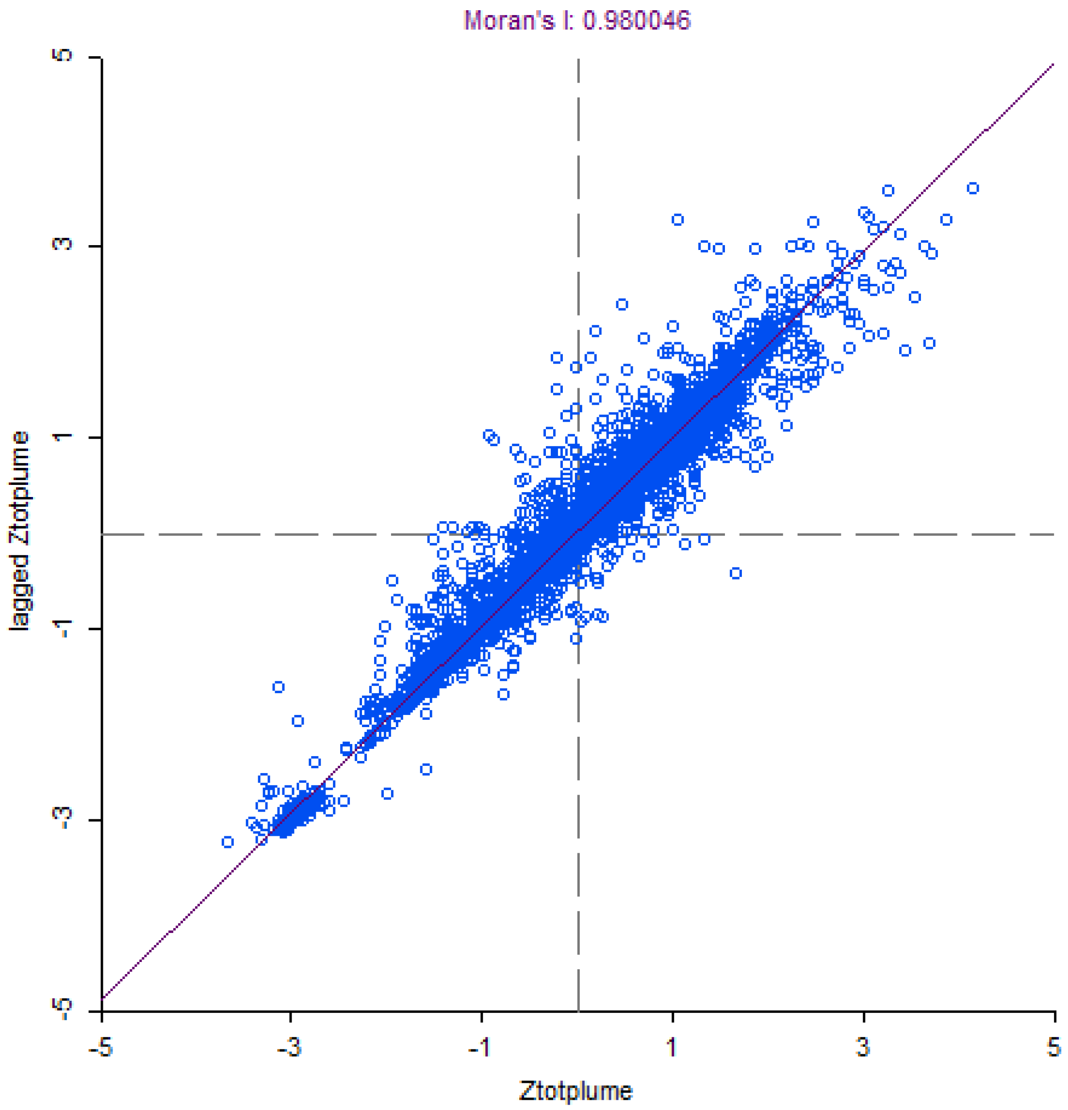
Next, we examined the association between SOVU and PLUME, again at the aggregate level, looking for an indication of spatial autocorrelation, using the global Moran’s I statistic (software GeoDaTM 1.6.61). Global Moran’s I is an indicator of aggregate spatial clustering (or dispersion). Values range between −1 (perfect dispersion) and +1 (perfect correlation). A value of zero indicates no spatial autocorrelation or a random spatial pattern. Table 3 shows results very similar to those for the r statistic for both the cooler and warmer months. All spatial analyses were conducted on z-scores for SOVU and PLUME.
The univariate, global Moran’s I values were also computed for SOVU and PLUME, respectively. The univariate indicator provides a measure of how well a variable clusters (or disperses) with itself. In Table 3, the values for SOVU across all regions suggest a considerable degree of spatial lag. In other words, we would expect to find either high socially vulnerable CBGs clustered together or low socially vulnerable clusters. The Moran’s I for PLUME shows near perfect autocorrelation for all regions in both seasons. To illustrate, Figure 2 and Figure 3 graph the global Moran’s I for SOVU (Mid-South) and PLUME (Mid-South spring/summer), respectively. In Figure 2, observations graphed in the top right quadrant indicate that high SOVU values in a given CBG i are surrounded by high SOVU values in neighboring CBGs; bottom left indicates that low SOVU observations in a CBG i are surrounded by low SOVU values in neighboring CBGs. The two spatial outlier quadrants are the low/high quadrant (top left) and bottom right (high/low).
Table 3. Pearson correlations and bivariate and univariate global Moran’s I for SOVU and PLUME by ecoregion and season of year.
EcoregionPearson Correlation (r)Bivariate Global Moran’s I (SOVU and PLUME)Univariate Global Moran’s I (SOVU)Univariate Global Moran’s I (PLUME)
WinterSpring/SummerWinterSpring/SummerWinterSpring/Summer
Appalachian-Cumberland (n = 8404)0.06 ***0.08 ***0.070.090.590.911.00
Piedmont (n = 12,103)0.06 ***0.19 ***0.070.200.650.940.99
Coastal Plain (n = 28,806)−0.14 ***−0.13 ***−0.13−0.130.630.930.98
Mississippi Alluvial (n = 2492)−0.24 ***−0.32 ***−0.23−0.300.540.920.92
Mid-South (n = 16,248)−0.14 ***−0.26 ***−0.13−0.250.690.920.98
*** p ≤ 0.0001.
Figure 2. Global Moran’s I for SOVU.
Forests 06 01397 g002
Figure 3. Global Moran’s I for PLUME.
Forests 06 01397 g003

4.2.2. LISA Bivariate Analysis

While Moran’s I indicates spatial clustering generally in the data, it does not reveal where this clustering appears across a study site. Again, a global statistic may conceal significant clustering. To determine how such clustering may manifest between two variables at the “local” level, we calculated the bivariate, local indicator of spatial association (LISA) statistic [35]. The analysis is based on the First Law of Geography which assumes that all things in space are related, but those things closer in space are more strongly related [30]. Therefore, we might expect certain social or biological/physical variables to cluster or hover together across space [24]. The null hypothesis in LISA analysis assumes that there is no spatial autocorrelation between the two variables examined. In other words, the relationship between two variables is random. However, if the null is rejected, this indicates that the relationship is not random, and that there is just a small chance (depending on the p-value) of obtaining the observed LISA statistic, if in the population the two variables are not co-located.
Spatial associations are based on clusters or the “neighborhood” of areal units adjacent to the areal unit of interest, i (in our case CBGs). We specified the neighborhood of CBG i based on a first order, queen contiguity weight matrix, which includes CBGs adjacent to CBG i that shared a common border length or vertex. Bivariate LISA is calculated by the equation from Sunderlin [30]:
I l = z x i j = 1 ,   j i N w i j   z y j  
where, Il is the LISA statistic; x is the SOVU value, and y is the PLUME value for CBG i and neighborhood j, respectively. Similarly, zx represents the standardized value for social vulnerability, and zy represents the standardized value for number of smoke plumes. The variable wij is the weight matrix that defines CBGs comprising neighborhood j (also generated using GeoDa™ 1.6.61). Because of difficulties in obtaining a LISA distribution, an ad hoc distribution is created each time the LISA analysis is performed. This is done by permutation of LISA values a specified number of times (e.g., 99, 999, 9999). Critical values are then selected for pseudo-p values. The LISA for a given CBG is compared with the critical value at a given significance level. For our analysis, significant clusters are those at the 0.05 level, with 999 permutations. Again, p values are presented for illustrative purposes.

4.2.3. Sub-Regional Results of Bivariate Analysis

In Figure 4, Figure 5, Figure 6, Figure 7, Figure 8, Figure 9, Figure 10, Figure 11, Figure 12 and 
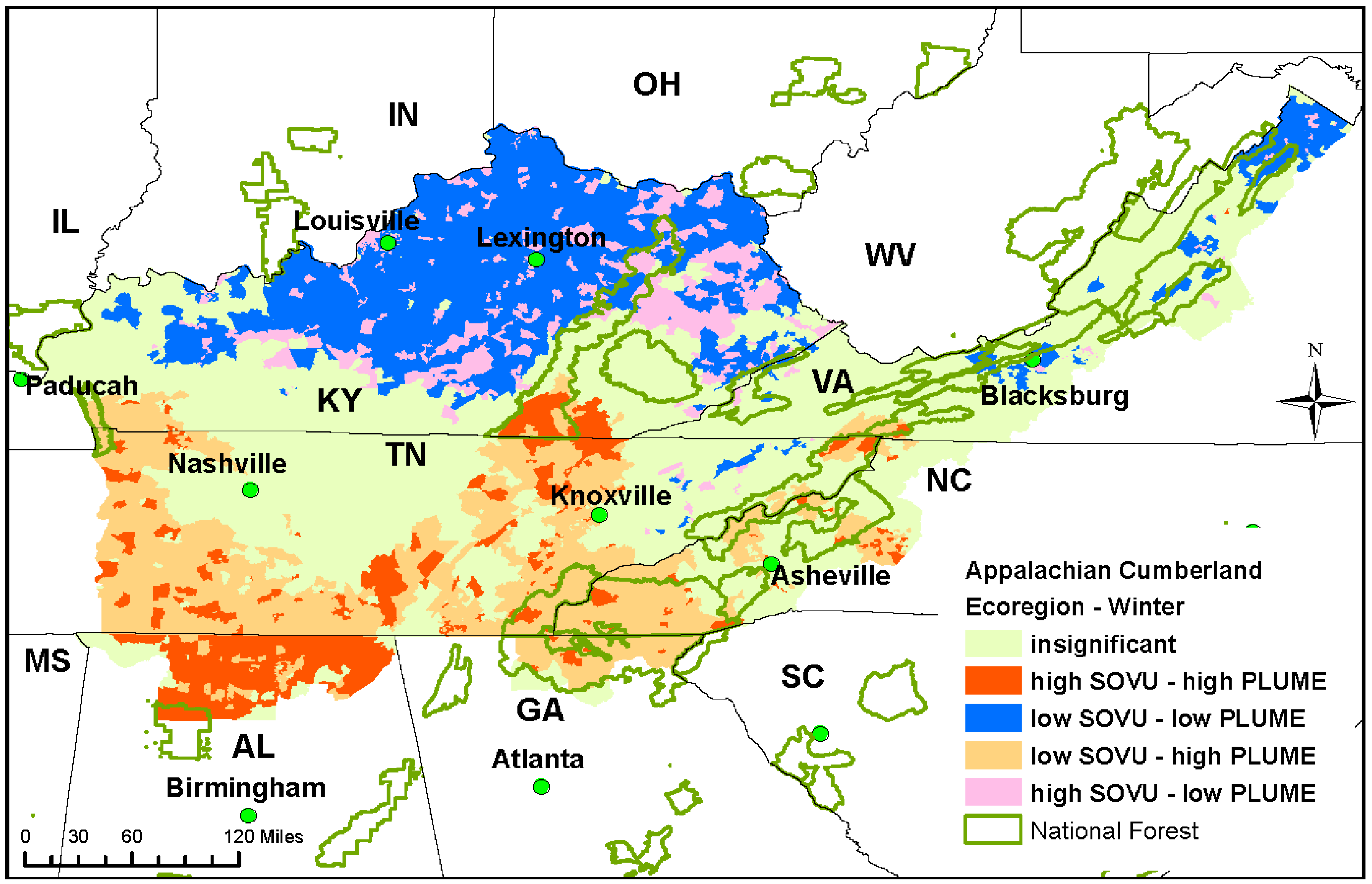
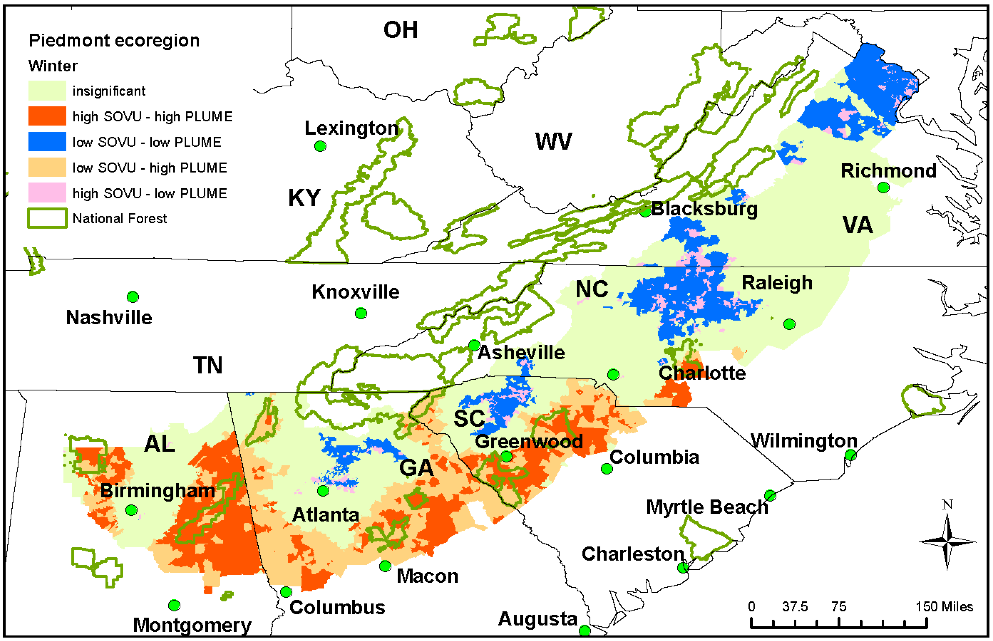
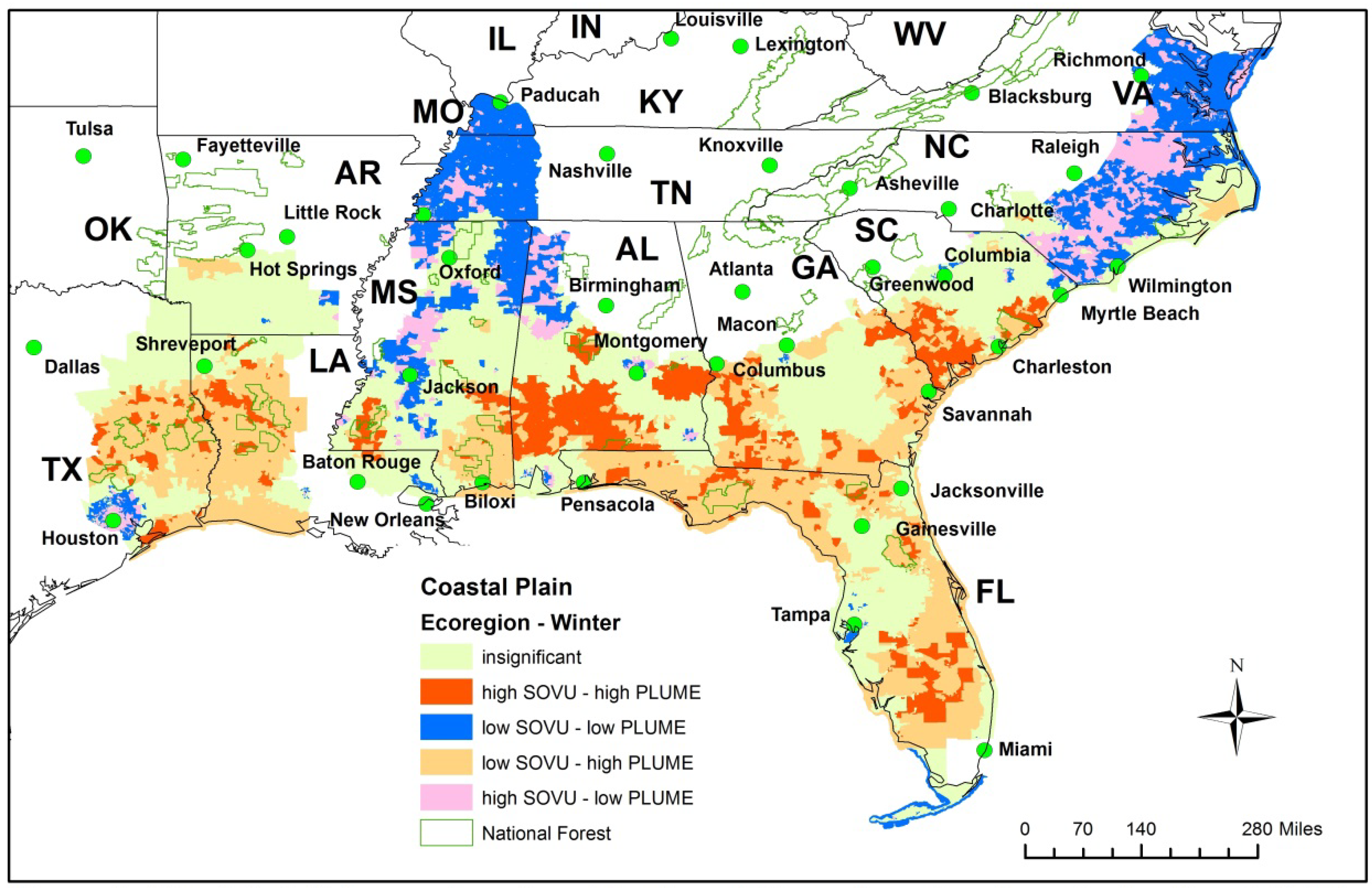
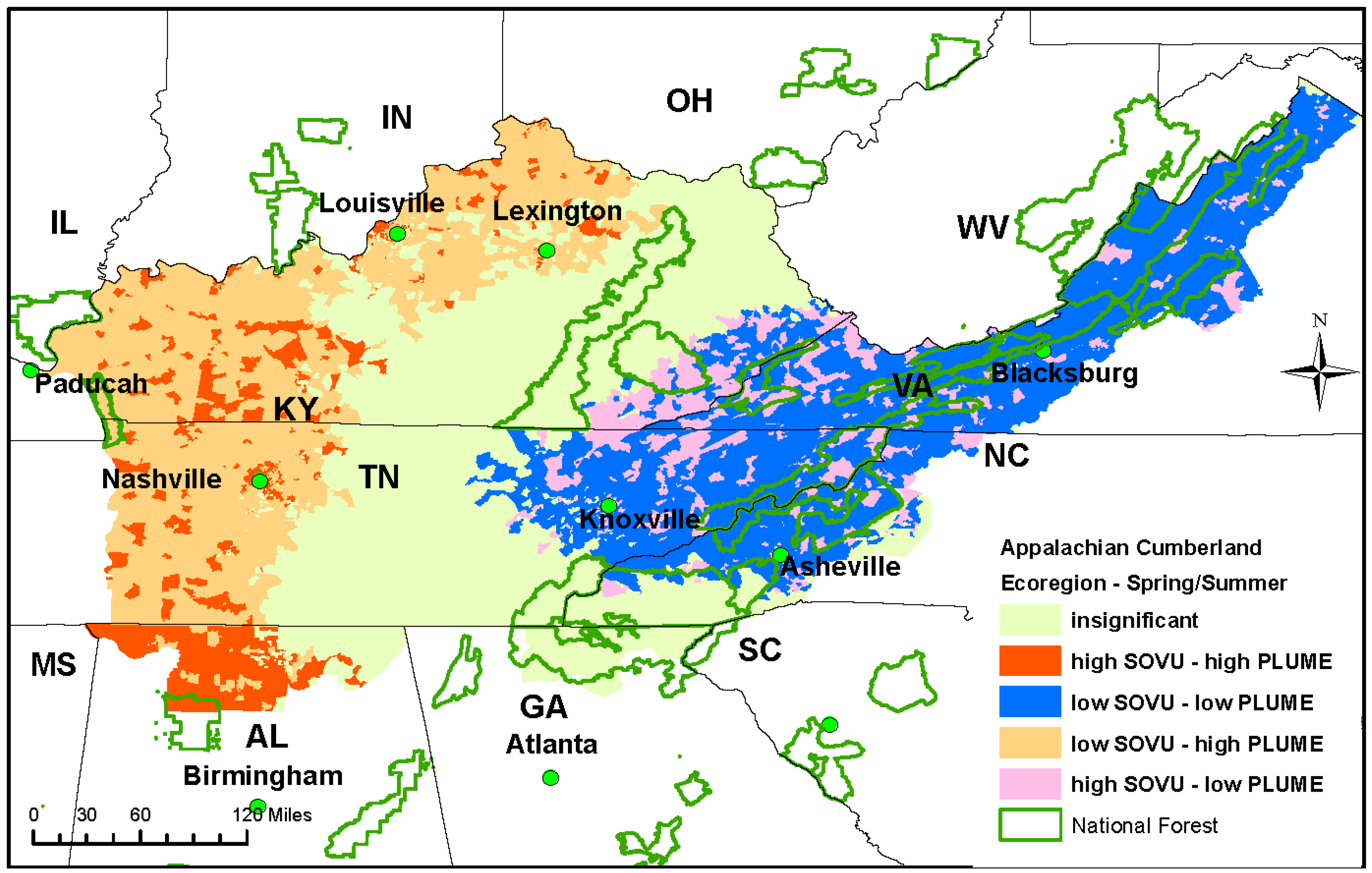
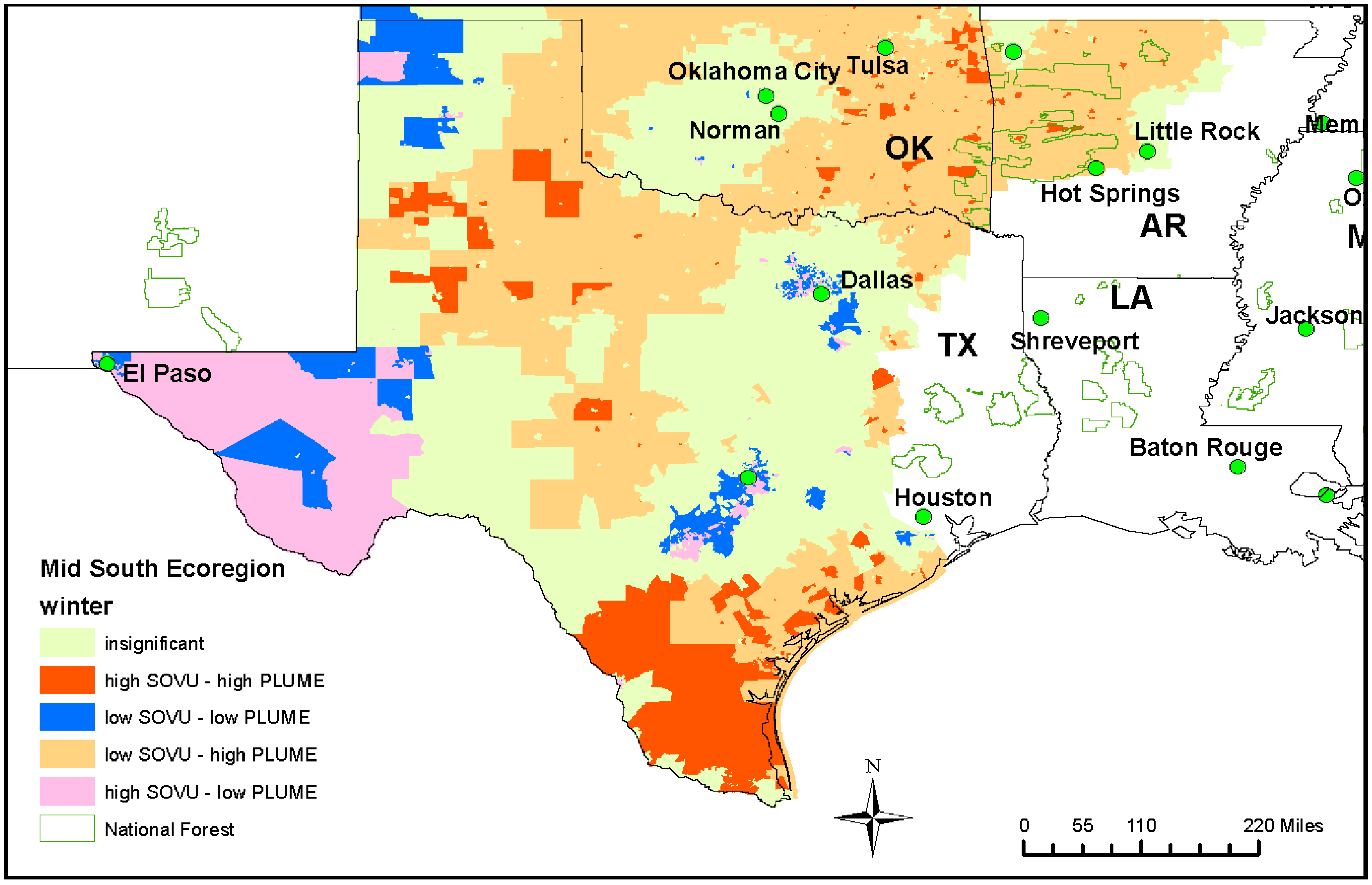
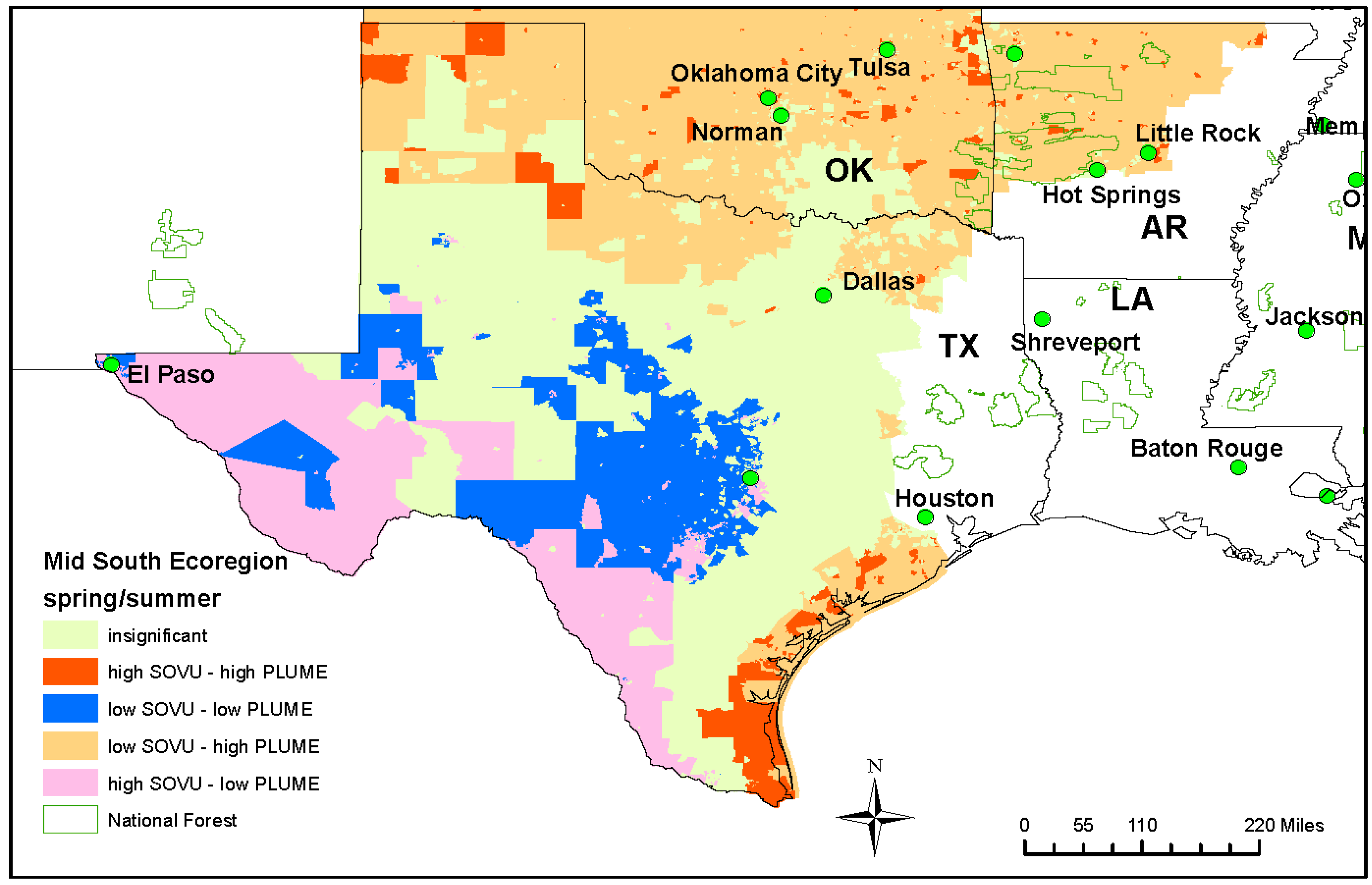
Figure 13, the LISA cluster mapping shows significant values for SOVU and PLUME grouped into four distinct clusters. These associations are described as either: high-high (high SOVU/high PLUME or “hot spots”); low-low (low SOVU/low PLUME or “cold spots”); low SOVU/high PLUME; or high SOVU/low PLUME. The low/high (green) and high/low (yellow) clusters are spatial outliers, meaning that the pattern is significant but the high and low values are intermixed. The high/low designation for each cluster (hotspot, coldspot, outlier) is determined by comparing the observed value of x or y for a given CBG with the average value of the respective variable for the entire study area (e.g., ecoregion [35]. For example, a high/high cluster in the Piedmont region shows CBGs with a higher than Piedmont average SOVU value surrounded by CBGs with a higher than Piedmont average PLUME value. Similarly, a low/low cluster in the Mid-South indicates CBGs with a lower than Mid-South average SOVU value surrounded by CBGs with lower than Mid-South average PLUME values. CBG boundaries are not displayed in order to help presentation clarity.
Figure 4. Bivariate LISA mapping of social vulnerability and smoke plume in the Appalachian-Cumberland ecoregion—winter.
Forests 06 01397 g004
Figure 5. Bivariate LISA mapping of social vulnerability and smoke plume in the Appalachian-Cumberland ecoregion—spring/summer.
Forests 06 01397 g005
Figure 6. Bivariate LISA mapping of social vulnerability and smoke plume in the Piedmont ecoregion—winter.
Forests 06 01397 g006
Figure 7. Bivariate LISA mapping of social vulnerability and smoke plume in the Piedmont ecoregion—spring/summer.
Forests 06 01397 g007
Figure 8. Bivariate LISA mapping of social vulnerability and smoke plume in the Coastal Plain ecoregion—winter.
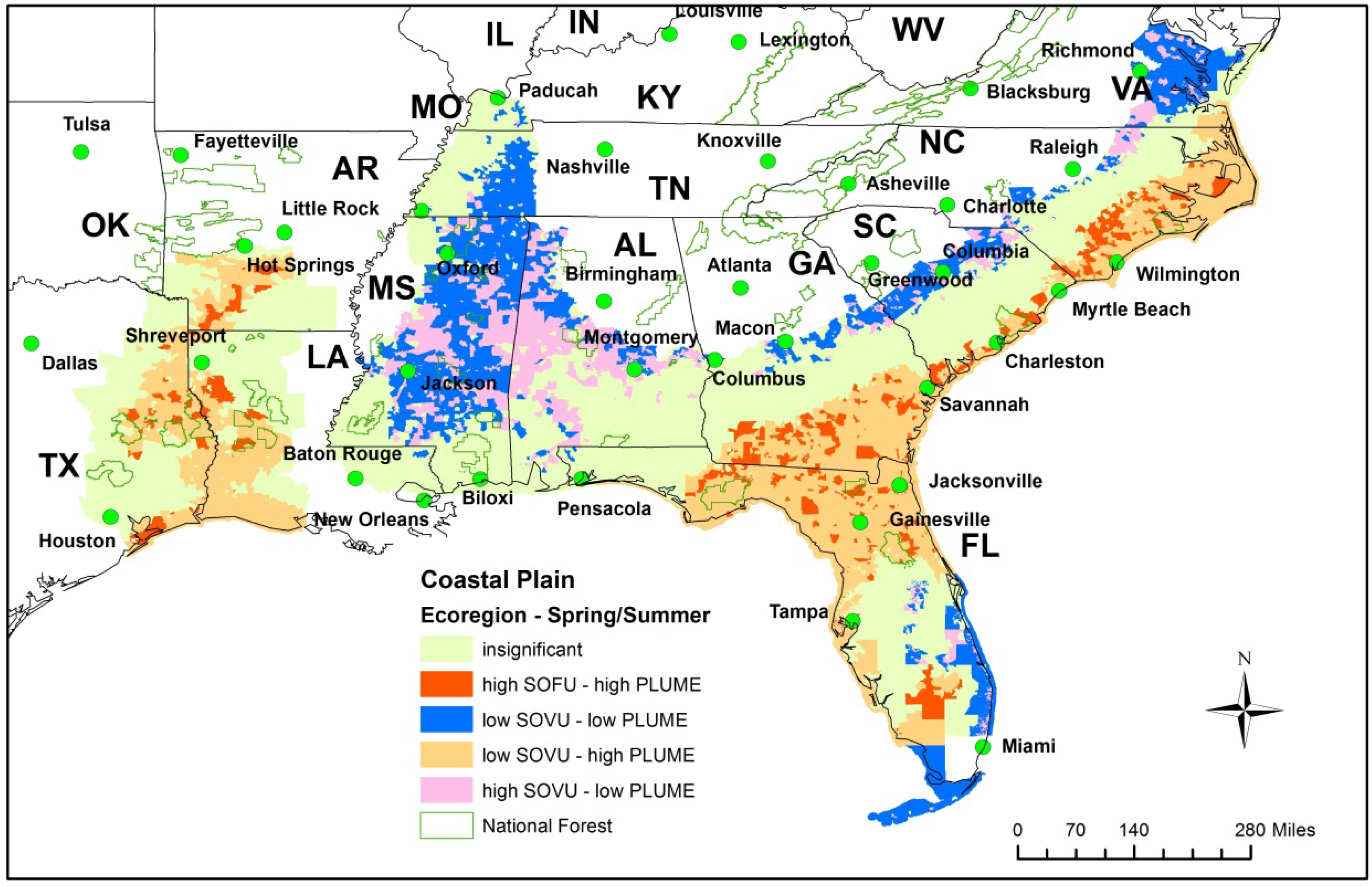
Forests 06 01397 g008
Figure 9. Bivariate LISA mapping of social vulnerability and smoke plume in the Coastal Plain ecoregion—spring/summer.
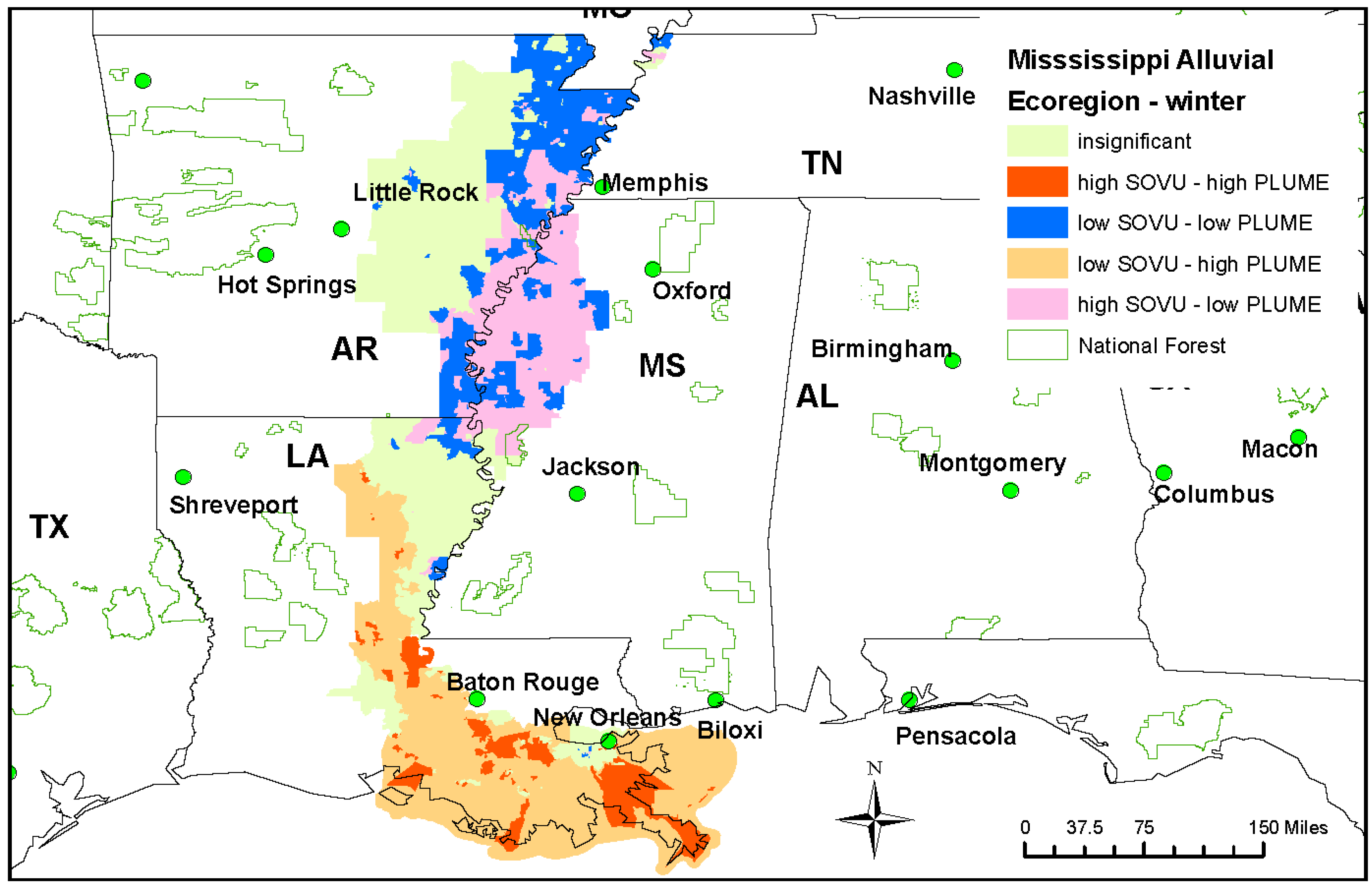
Forests 06 01397 g009
Figure 10. Bivariate LISA mapping of social vulnerability and smoke plume in the Mississippi-Alluvial ecoregion—winter.
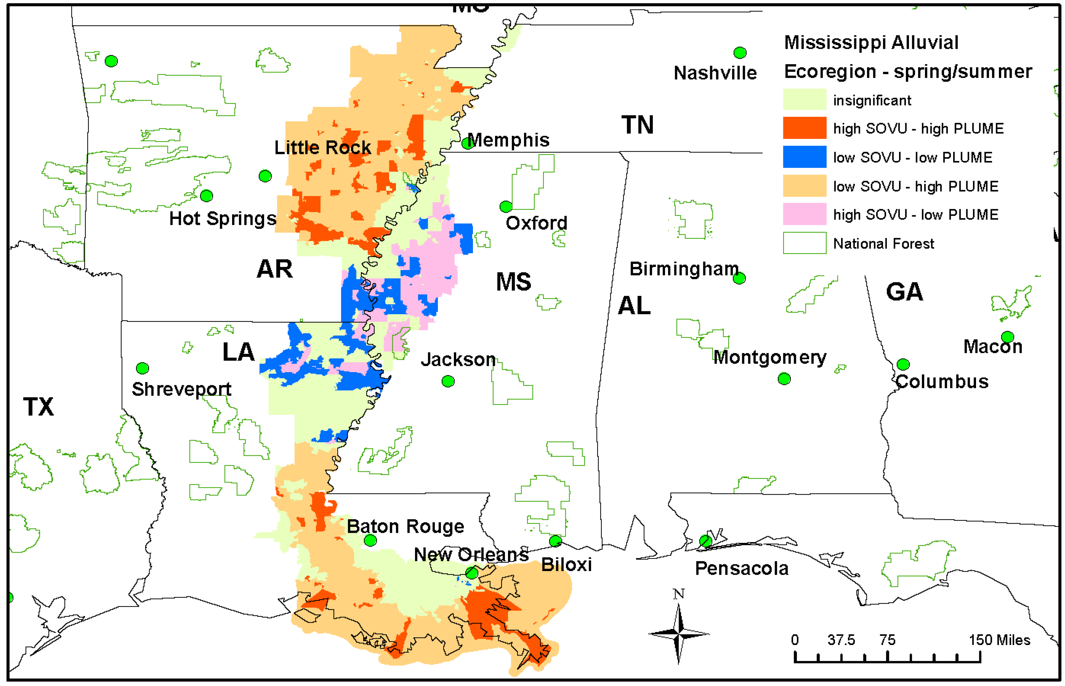
Forests 06 01397 g010
Figure 11. Bivariate LISA mapping of social vulnerability and smoke plume in the Mississippi-Alluvial ecoregion—spring/summer.
Forests 06 01397 g011
Figure 12. Bivariate LISA mapping of social vulnerability and smoke plume in the Mid-South ecoregion—winter.
Forests 06 01397 g012
Figure 13. Bivariate LISA mapping of social vulnerability and smoke plume in the Mid-South ecoregion—spring/summer.
Forests 06 01397 g013

Appalachian-Cumberland

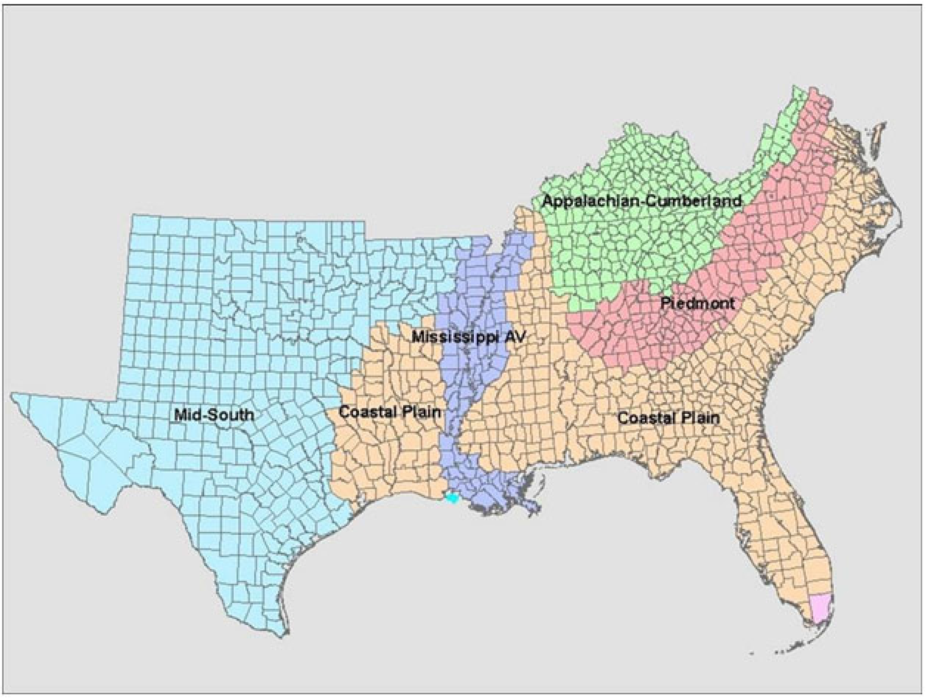
The Appalachian-Cumberland ecoregion stretches from northern Virginia to western Kentucky, Tennessee, and north Alabama, covering an area of 99 million square miles. Figure 4 and Figure 5 illustrate bivariate LISA clusters for the Appalachian-Cumberland highlands. The winter month clusters (Figure 4) show hot spots occurring in northern Alabama and in the 180 mile stretch between Knoxville and Nashville, TN. The William B. Bankhead National Forest (NF) in Alabama overlaps a portion of the hot spot. The Chattahoochee NF in north Georgia and the Cherokee NF just over the border in Tennessee overlap with both hot spots and outlier clusters at the Georgia-Tennessee line. Further to the northeast, hot spots can be seen near Asheville, NC, again overlapped by or proximal to National Forest lands (the Pisgah in North Carolina). There is also substantial intersection between the Daniel Boone NF in eastern Kentucky and hot spot clusters.
Hot and cold spots shift geographies in the spring and summer months, relative to the winter (Figure 5). Hot spots are seen most clearly in the extreme western part of the Appalachian-Cumberland region in the warm season, and cold spots are in the central and northeastern most reaches of the ecoregion at this time. There is extensive overlap of cold spots with National Forests in the eastern Appalachian-Cumberland area but only small intersections in the western part of this ecoregion.

Piedmont

In the Piedmont during winter months, hot spots are evident in north Alabama (overlapping with the Talladega and Bankhead NFs), east and west of Birmingham. Hot spots are interspersed with low social vulnerability/high plume counts in Georgia in an area north of Macon and Columbus. Portions of the Chattahoochee-Oconee NF are proximal to these hot spots. In South Carolina, hot spots are clustered near Greenwood and in an area interspersed with low social vulnerability/high plume counts near the Sumpter NF. Hot spots also cluster southeast of Charlotte, NC, overlapping with the boundaries of the Uwharrie NF. Cold spots in winter months lie mostly to the north of hot spots throughout the Piedmont. A similar distribution of hot and cold spots is seen during the spring/summer season in the Piedmont, although there is a larger clustering of significant hot spots in Alabama. Also, hot spots appear just north of Raleigh, NC during the warmer season.

Coastal Plain

The Coastal Plain extends from southern Virginia, through Georgia and Alabama, and into Louisiana and east Texas—an area of more than 79 million square miles. In winter, hot spots converge to the north and south of Charleston, SC, and in a swath between Columbia, SC and Savannah, GA. The Francis Marion NF in South Carolina abuts hot spots in both winter and spring/summer. An inverted arc of hot spots and low/high clusters occur in South Georgia. Larger hot spot clusters congregate throughout south Alabama in winter. In terms of social vulnerability, hot spot clusters in this ecoregion are consistent with prior mappings of southern Black Belt counties and the concomitant generational poverty pervading some of these counties, particularly during the winter season [36]. As expected, above average plume activity predominate in large areas of Florida in both winter and spring/summer. Hot spots also occur near the Ocala and Apalachicola, NF in Florida. Moving west, Figure 8 shows hot spots interspersed with low/high clusters between Shreveport, LA and Houston, TX. In Louisiana, portions of the Kisatchie NF are interspersed with hot spots.
In warmer months, hot spot activity shifts to the extreme eastern part of the region, from eastern North Carolina down to an area south of Jacksonville, FL. Hot spot CBGs are also prominent in South Georgia, north central Florida and south Florida. Sporadic hot spot scatterings also appear in southern Louisiana up to an area below Hot Springs, AR. Large cold spot clusters occur east of Oxford, MS and Memphis, TN and east of Jackson, MS.

Mississippi Alluvial Valley

The Mississippi Alluvial Valley originates at the confluence of the Ohio and Mississippi Rivers in southern Illinois and runs to the Gulf of Mexico. In winter, hot spots occur near Baton Rouge and New Orleans, LA. Cold spots occur north of Jackson, MS up through Memphis, TN. In summer, hot spot activity is seen in the north and south of the region.

Mid-South

The Mid-South ecoregion covers most of Texas, all of Oklahoma and much of northwestern Arkansas. In winter, hot spot clusters are prominent in the south Texas. Hot spots are also seen in northwest Texas and in east Oklahoma and west Arkansas. The Ozark National Forest is proximal to some of the hot spot clusters in this part of the Mid-South. During the warmer months, hot spots are also in the very southern tip of Texas and are scattered throughout the northern part of the ecoregion.
In sum, the LISA analysis identified four significant clusters or associations between social vulnerability and plume dispersion across the South. While we did find “hot spots,” they do not characterize the relationship between these variables, overall. To help clarify this relationship, Table 4 and Table 5 show the distribution of association types in each region, by season. The majority of associations between social vulnerability and smoke plume are not significant at p ≤ 0.05 in winter or in the Coastal Plain, Mississippi Alluvial, and Mid-South in spring/summer. In fact, the significant high/high associations accounted for no more than 8 percent of all associations in any ecoregion in winter (Appalachian Cumberland) and roughly 16 percent in spring/summer (Piedmont).

4.2.4. Plume Intensity in Hot Spots and Low/High Clusters

Next, we compared the intensity of plume exposure for hot spots and low/high smoke plume clusters by calculating the mean number of plumes for both cluster types. As well, we present the total number of clusters for both hot spots and low/high clusters. We also compared the mean number of plumes for hot spots and low/high clusters within one mile of a National Forest.
We compared hot spots and low/high clusters because these clusters controlled for smoke exposure. Both cluster types had “high” (above average) smoke exposure, only social vulnerability varied. The idea was to see if socially marginal clusters with high smoke exposure experienced more smoke compared to non-socially marginal populations with high smoke exposure in general and for clusters proximal to National Forests.
Table 4. Distribution of LISA Clusters by Ecoregion—Winter.
Type of AssociationAppalachian Cumberland (N = 8404)Piedmont (N = 12,103)Coastal Plain (N = 28,806)Mississippi Alluvial (N = 2492)Mid-South (N = 16,248)
CBG (%)CBG (%)CBG (%)CBG (%)CBG (%)
High/High8.025.214.474.254.92
Low/Low18.2119.1914.039.7911.97
Low/High10.575.348.6012.9610.85
High/Low11.8210.1114.8513.3615.05
Insignificant51.3961.1658.0559.6357.21
Total100.00100.00100.00100.00100.00
Table 5. Distribution of LISA Clusters by Ecoregion—Spring/Summer.
Type of AssociationAppalachian Cumberland (N = 8404)Piedmont (N = 12,103)Coastal Plain (N = 28,806)Mississippi Alluvial (N = 2492)Mid-South (N = 16,248)
CBG (%)CBG (%)CBG (%)CBG (%)CBG (%)
High/High14.1615.624.904.497.82
Low/Low20.5919.7413.386.228.40
Low/High19.3413.2712.4716.5317.10
High/Low11.177.5310.949.8712.60
Insignificant34.7643.8457.2462.8854.07
Total100.00100.00100.00100.00100.00
Table 6. Mean plume count in hot spot and low/high clusters generally and within 1 mile of a National Forest. Number of hot spots and low/high clusters generally and within 1 mile of a National Forest—winter.
EcoregionMean Number of Plumes in Hot SpotsMean Number of Plumes in Low/High ClustersNumber of Hot SpotsNumber of Low/High ClustersMean Number of Plumes in hot Spots near National Forest Mean Number of Plumes in Low/High Clusters near National ForestsNumber of Hot Spots near National ForestsNumber of Low/High clusters near National Forests
Appalachian Cumberland6.90 (s.d. = 3.48)6.32 (s.d. = 2.66)6748889.19 (s.d. = 7.55)8.19 (s.d. = 3.94)75206
Piedmont21.70 (s.d. = 11.86)21.91 (s.d. = 12.43)63064628.34 (s.d. = 16.10)26.81 (s.d. = 18.43)124127
Coastal Plain47.09 (s.d. = 21.93)50.98 (27.04)1255241465.73 (s.d. = 33.72)71.28 (37.15)97292
Mississippi Alluvial23.31 (s.d. = 6.60)25.13 (s.d. = 8.18)1063230000
Mid-South21.80 (s.d. = 9.90)25.64 (s.d. = 12.74)799176336.00 (s.d. = 15.59)40.61 (s.d. = 17.36)15145
Table 7. Mean plume county in hot spot and low/high clusters generally and within 1 mile of a National Forest. Number of hot spots and low/high clusters generally and within 1 mile of a National Forest—spring/summer.
EcoregionMean Number of Plumes in Hot SpotsMean Number of Plumes in Low/High ClustersNumber of Hot SpotsNumber of Low/High ClustersMean Number of Plumes in Hot Spots near National Forest Mean Number of Plumes in Low/High Clusters near National ForestsNumber of Hot Spots near National ForestsNumber of Low/High Clusters near National Forests
Appalachian Cumberland87.75 (s.d. = 4.23)87.92 (s.d. = 5.18)1190162595.83 (s.d. = 2.97)99.38 (s.d.8.18)68
Piedmont90.21 (s.d. = 4.92)91.49 (s.d. = 4.62)1891160694.85 (s.d. = 7.90)93.54 (s.d. = 6.18)11068
Coastal Plain160.89 (s.d. = 22.60)162.05 (s.d. = 27.01)14113593163.08 (s.d. = 23.25)164.22 (s.d. = 26.64)61199
Mississippi Alluvial136.90 (s.d. = 8.42)139.61 (s.d. = 9.56)112412013501
Mid-South140.24 (s.d. = 9.28)139.38 (s.d. = 8.9312712778135.80 (s.d. = 5.34)140.17 (s.d. = 6.39)10138
Table 6 contains results for the winter season. Mean number of plumes was slightly higher in hot spots, compared to low/high areas for the Appalachian Cumberland ecoregion, in general, and for areas near National Forests in that ecoregion. Otherwise, hot spots were not more encumbered by smoke than other places across the South. Also, the number of hot spots near National Forests is either less than or equal (Mississippi-Alluvial) to the number of low/high clusters. Table 7 also shows overwhelmingly that there is not more smoke exposure in hot spots vis-à-vis low/high clusters during the warmer months. Overall, results do not suggest that socially vulnerable populations are potentially exposed to more smoke plumes than populations that are not vulnerable in the terms we measured.

5. Conclusions

This exploratory study provides a baseline assessment of the spatial intersection between an indicator of social vulnerability and population exposure to smoke pollution at the CBG level across the U.S. South. Again, while we did find significant spatial clustering of high social vulnerability block groups in the vicinity of block groups with a high number of smoke plumes, this type of association does not predominate in any of the ecoregions. Therefore, we cannot conclude that socially vulnerable populations in the region, overall, are exposed to more smoke from wildfires and prescribed fires, compared to communities that are not socially vulnerable.
Ours is the first analysis to assess this relationship at a broad scale; as such, it provides a point of departure for subsequent studies examining community-level exposure to smoke from both wildfire and prescribed fire. Data presentation at this stage is more descriptive than quantitative, as the LISA analysis indicated hot or cold spot clusters based on a given CBG’s value relative the mean. While a given PLUME score may be greater than the neighborhood mean, smoke may pose little threat to public health. The present analysis allowed us to examine only potential smoke exposure, rather than actual exposure because we did not examine how much particulate matter (PM < 2.5) was distributed on the ground. With respect to impacts from exposure, we also had no data indicating actual impacts to human health; for example, population-level responses in terms of hospital admittance or other emergency treatments [20].
Further, policy implications from this study are limited because we were not able to discern fire source (wildland or prescribed burn). Subsequent studies should examine smoke dispersal from prescribed burns initiated by publicly-managed agencies to assess the impact of such fires on vulnerable populations. Federal agencies are mandated by Executive Order 12898 to examine the impacts of their policies and programming on minority and low income populations. Such studies would have a direct bearing on federal agencies’ responsibilities to both manage fuel reductions and to help ensure the health and safety of affected populations.

Acknowledgments

The authors acknowledge the helpful contribution of Stanley Zarnoch regarding data manipulation and statistical advice. We also thank Marilyn G. Howard for helping to tabulate wildfire data from the National Interagency Fire Center for the southern U.S. and Shela Mou for map formatting.

Author Contributions

Cassandra Johnson Gaither conceptualized the article, conducted the statistical analyses, and wrote the analysis and concluding sections. Scott Goodrick assembled and scaled the plume data to the census block group level and provided a description of the methods used to obtain the plume data and discussions of fire behavior. Bryn Elise Murphy conducted the literature review on human vulnerability to smoke, and Neelam Poudyal provided critical review of the document and advice on the LISA analysis.

Conflicts of Interest

The authors declare no conflict of interest.

References

  1. Fowler, C.; Konopik, E. The history of fire in the southern United States. Hum. Ecol. Rev. 2007, 14, 165–176. [Google Scholar]
  2. Stanturf, J.A.; Wade, D.W.; Waldrop, T.A.; Kennard, D.K.; Achtemeier, G.L. Background Paper Fire: Fire in Southern Forest Landscapes; USDA Forest Service Southern Research Station: Asheville, NC, USA, 2002. [Google Scholar]
  3. Monroe, M.C. Fire. Human Influences on Forest Ecosystems: The Southern Wild-Land Urban Interface Assessment; GTR SRS-55; Macie, E.A., Hermansen, L.A., Eds.; USDA Forest Service Southern Research Station: Asheville, NC, USA, 2002; pp. 133–150. [Google Scholar]
  4. Achtemeier, G.L.J.B.; Brenner, J.D. Problem and Nuisance Smoke. Smoke Management Guide for Prescribed and Wildland Fire: 2001 Edition; National Interagency Fire Center: Boise, ID, USA, 2001; pp. 41–49. [Google Scholar]
  5. Kelly, P.M.; Adger, W.N. Theory and practice in assessing vulnerability to climate change and facilitating adaptation. Clim. Chang. 2000, 47, 325–352. [Google Scholar] [CrossRef]
  6. U.S. General Accounting Office. Siting of Hazardous Waste Landfills and Their Correlation with Racial and Economic Status of Surrounding Communities; U.S. General Accounting Office: Gaithersburg, MD, USA, 1983; p. 13. [Google Scholar]
  7. Bullard, R.D. Dumping in Dixie: Race, Class, and Environmental Quality; Westview Press: Boulder, CO, USA, 1990. [Google Scholar]
  8. Mohai, P.; Saha, R. Racial inequality in the distribution of hazardous waste: A national-level reassessment. Soc. Pro. 2007, 54, 343–370. [Google Scholar] [CrossRef]
  9. Pastor, M., Jr.; Sadd, J.L.; Morello-Frosch, R. Waiting to inhale: The demographics of toxic air release facilities in 21st-century California. Soc. Sci. Q. 2004, 85, 420–440. [Google Scholar] [CrossRef]
  10. Sadd, J.L.; Pastor, M.; Morello-Frosch, R.; Scoggins, J.; Jesdale, B. Playing it safe: Assessing cumulative impact and social vulnerability through an environmental justice screening method in the south coast air basin, California. Int. J. Res. Public Health 2011, 8, 1441–1459. [Google Scholar] [CrossRef]
  11. Makri, A.; Stilianakis, N.I. Vulnerability to air pollution health effects. Int. J. Hyg. Environ. Health 2008, 211, 326–336. [Google Scholar] [CrossRef] [PubMed]
  12. Collins, T.W. Households, forests, and fire hazard vulnerability in the American West: A case study of a California community. Glob. Environ. Chang. Part B Environ. Hazards 2005, 6, 23–37. [Google Scholar]
  13. Collins, T.W. The political ecology of hazard vulnerability: Marginalization, facilitation and the production of differential risk to urban wildfires in Arizona’s White Mountains. J. Polit. Ecol. 2008, 15, 21–43. [Google Scholar]
  14. Lynn, K.; Gerlitz, W. Mapping the Relationship between Wildfire and Poverty. In Proceedings of the Fuels Management-How to Measure Success, Portland, OR, USA, 28–30 March 2006; pp. 401–415.
  15. Ojerio, R.; Lynn, K.; Evans, A.; DeBonis, M.; Gerlitz, W. Engaging Socially Vulnerable Populations in Community Wildfire Protection Plans; University of Oregon: Eugene, OR, USA, 2008; p. 23. [Google Scholar]
  16. Andreu, A.; Hermansen-Baez, L. Fire in the South 2: The Southern wildfire Risk Assessment; The Southern Group of State Foresters: Gainesville, FL, USA, 2008; p. 32. [Google Scholar]
  17. Johnson Gaither, C.; Poudyal, N.; Goodrick, S.; Bowker, J.M.; Malone, S.; Gan, J. Wildland fire risk and social vulnerability in the Southeastern United States: An exploratory spatial data analysis approach. For. Policy Econ. 2011, 13, 24–36. [Google Scholar] [CrossRef]
  18. Macie, E.A.; Hermansen, L.A. Human Influences on Forest Ecosystems: The Southern Wildland-Urban Interface Assessment; GTR SRS-55; Macie, E.A., Hermansen, L.A., Eds.; USDA Forest Service Southern Research Station: Asheville, NC, USA, 2002; p. 159. [Google Scholar]
  19. Poudyal, N.C.; Johnson-Gaither, C.; Goodrick, S.; Bowker, J.M.; Gan, J. Locating spatial variation in the association between wildland fire risk and social vulnerability across six southern states. Environ. Manag. 2012, 49, 623–635. [Google Scholar] [CrossRef]
  20. Stewart, S.; Radeloff, V.; Hammer, R.; Fried, J.; Holcomb, S.; McKeefry, J. Mapping the Wildland Urban Interface and Projecting Its Growth to 2030: Summary Statistics; USDA Forest Service North Central Research Station: Evanston, IL, USA, 2005. [Google Scholar]
  21. Radeloff, V.C.; Hammer, R.B.; Stewart, S.I.; Fried, J.S.; Holcomb, S.S.; McKeefry, J.F. The wildland-urban interface in the United States. Ecol. Appl. 2005, 15, 799–805. [Google Scholar] [CrossRef]
  22. Hammer, R.B.; Stewart, S.I.; Radeloff, V.C. Demographic trends, the wildland-urban interface, and wildfire management. Soc. Nat. Resour. 2009, 22, 777–782. [Google Scholar] [CrossRef]
  23. Johnson Gaither, C.; Roberts, N.S.; Hanula, K.L. Visitor Diversity through the Recreation Manager Lens: Forest Service Regions 8 (U.S. South) and 5 (California); USDA Forest Service: Asheville, NC, USA, 2015; p. 22. [Google Scholar]
  24. Sunderlin, W.D.; Dewi, S.; Puntodewo, A.; Muller, D.; Angelsen, A.; Epprecht, M. Why forests are important for global poverty alleviation: A spatial explanation. Ecol. Soc. 2008, 13, 24. [Google Scholar]
  25. National Interagency Fire Center. Historical Year-End Fire Statistics by State (Source NICC); National Interagency Fire Center: Boise, ID, USA, 2014. [Google Scholar]
  26. U.S. Census Bureau. State Area Measurements and Internal Point Coordinates. Available online: https://www.census.gov/geo/reference/state-area.html (accessed on 4 October 2014).
  27. Naeher, L.P.; Brauer, M.; Lipsett, M.; Zelikoff, J.T.; Simpson, C.D.; Koenig, J.Q.; Smith, K.R. Woodsmoke health effects: A review. Inha. Toxi. 2007, 19, 67–106. [Google Scholar] [CrossRef]
  28. Core, J.E. Visibility. In Smoke Management Guide for Prescribed and Wildland Fire, 2001 ed.; Hardy, C.C., Ed.; National Interagency Fire Center: Boise, ID, USA, 2001; pp. 35–39. [Google Scholar]
  29. Abdel-Aty, M.; Ekram, A.-A.; Huang, H.; Choi, K. A study on crashes related to visibility obstruction due to fog and smoke. Accid. Anal. Prev. 2011, 43, 1730–1737. [Google Scholar] [CrossRef] [PubMed]
  30. Wear, D.N. Forecasts of land uses. In The Southern Forest Futures Project; Wear, D.N., Greis, J.G., Eds.; USDA Forest Service Southern Research Station: Asheville, NC, USA, 2014; pp. 123–178. [Google Scholar]
  31. Johnson-Gaither, C.; Schelhas, J.; Zipperer, W.; Sun, G.; Caldwell, P.; Poudyal, N. Water Stress and Social Vulnerability in the Southern United States, 2010–2040. In Climate Change Adaptation and Mitigation Management Options; Vose, J.M., Klepzig, K.D., Eds.; CRC Press; Taylor & Francis Group: Boca Raton, FL, USA, 2014; pp. 61–83. [Google Scholar]
  32. U.S. Census Bureau. Census of Population and Housing. 2010 Census Summary File 1. Accessed through Social Explorer Tables (SE) Age: T8, Race: T54, Hispanic or Latino Origin by Race: T55, Tenure: T69; U.S. Census Bureau: Washington, DC, USA, 2011. [Google Scholar]
  33. U.S. Census Bureau. American Factfinder. Table C17002, Ratio of Income to Poverty Level in the Past 12 Months. Available from 2006 to 2010 American Community Survey Five Year Estimates Data Downloaded with Summary File Retrieval Tool for the American Community Survey. 2011. Available online: https://www.socialexplorer.com/data/ACS2010/metadata/?ds=American+Community+Survey+2010&table=C17002 (accessed on 10 July 2013).
  34. Gwynn, R.C.; Thurston, G.D. The Burden of air pollution: Impacts among racial minorities. Environ. Health Perspect. 2001, 109, 501–506. [Google Scholar] [CrossRef] [PubMed]
  35. Anselin, L. Local indicators of spatial association-LISA. Geogr. Anal. 1995, 27, 93–115. [Google Scholar] [CrossRef]
  36. Wimberley, R.C. The Southern Black Belt: A National Perspective; Southern Rural Development Center: Starkville, MS, USA, 1997; p. 49. [Google Scholar]

