Sensitivity Analysis of 3D Individual Tree Detection from LiDAR Point Clouds of Temperate Forests


Abstract
:1. Introduction
2. Methodology
2.1. Single Tree Detection
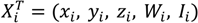 is provided for each reflection i with the 3D coordinates of the echo. Additionally, the points Xi are given by the width Wi and the intensity Ii of the echo pulse [5]. The LiDAR data are corrected by referencing Wi and Ii to the pulse width and the intensity of the emitted Gaussian pulse and by correcting the intensity with respect to the run length Si (distance between laser sensor and target) of the laser beam and a nominal distance.
 . Based on bilinear interpolation, the ground level is estimated from a given digital terrain model (DTM) with a grid size of 1 m and an absolute accuracy of 25 cm [11]. In the next step, all the highest 3D points
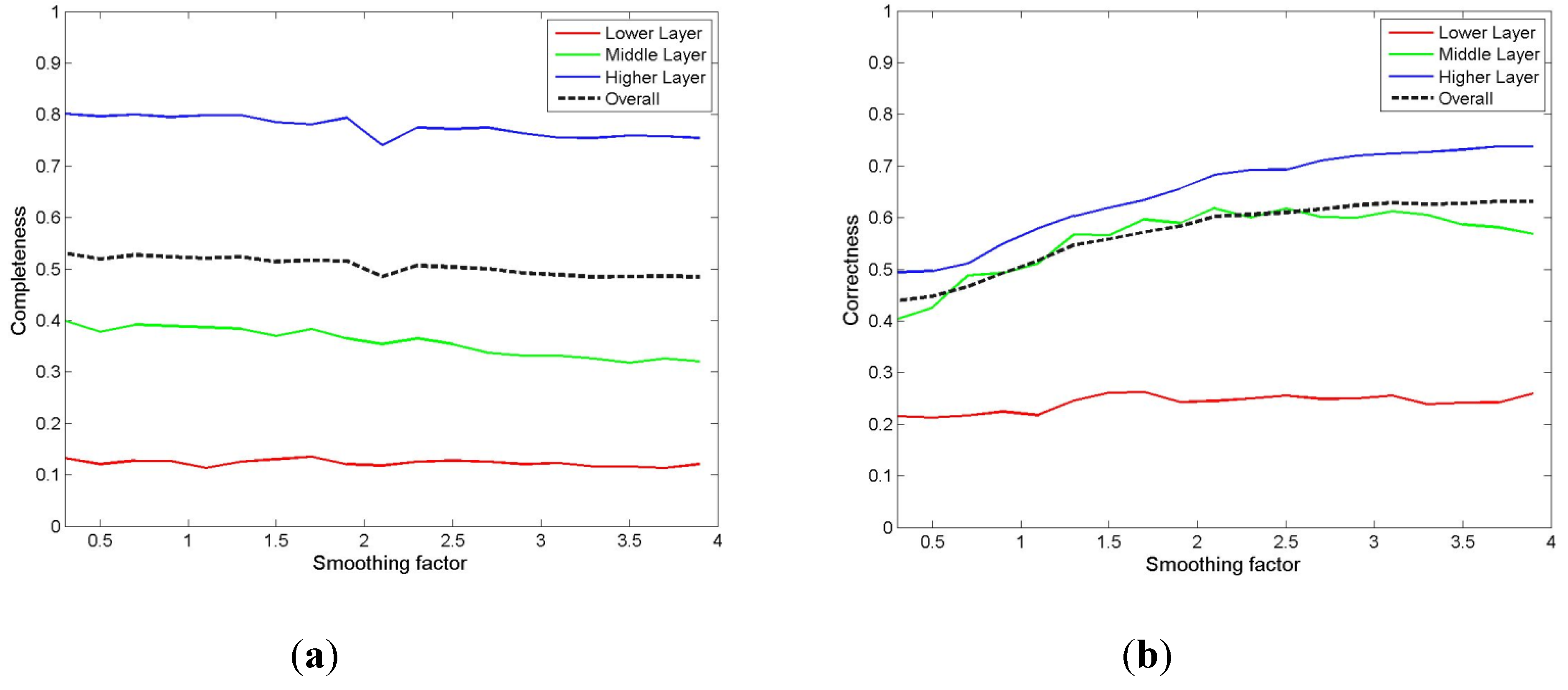
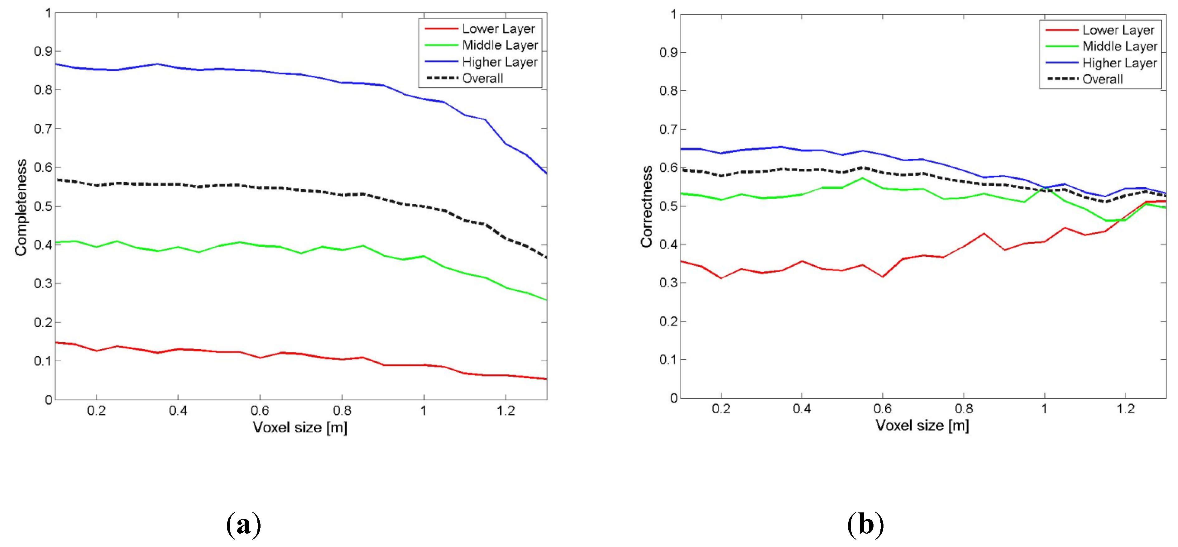
  of all NC cells are robustly interpolated in a grid that has NX and NY grid lines and a grid size gw. For this purpose an algorithm “gridfit” [26] is adopted which smoothens the surface by maintaining the surface gradients as small as possible. The trade-off between interpolation and regularization is determined by the adjustable smoothing factor λ. Both steps are carried out simultaneously in a least squares adjustment. The watershed segments derived on this CHM act as candidate regions where single trees are contained.
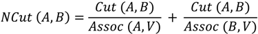

 that computes the similarities wij between two voxels i and j within a cylinder of radius rxy around the voxel i. The components X(I,j) and Z(i,j) weight quadratic horizontal and vertical Euclidian distances between voxels. They are weighted separately to take into account information about the typical tree shape. The component F(i,j) describes the quadratic Euclidian distance between two feature vectors (mean pulse intensity Imean and pulse width Wmean) derived from the data points (=reflections) in the voxels. The fraction G(I,j) models the dependency of two voxels i and j of the local maxima by the maximal horizontal distance
  . Hence, it is modeled that voxels nearby belong most probably belong to one tree.
2.2. Key Control Parameters for Sensitivity Analysis
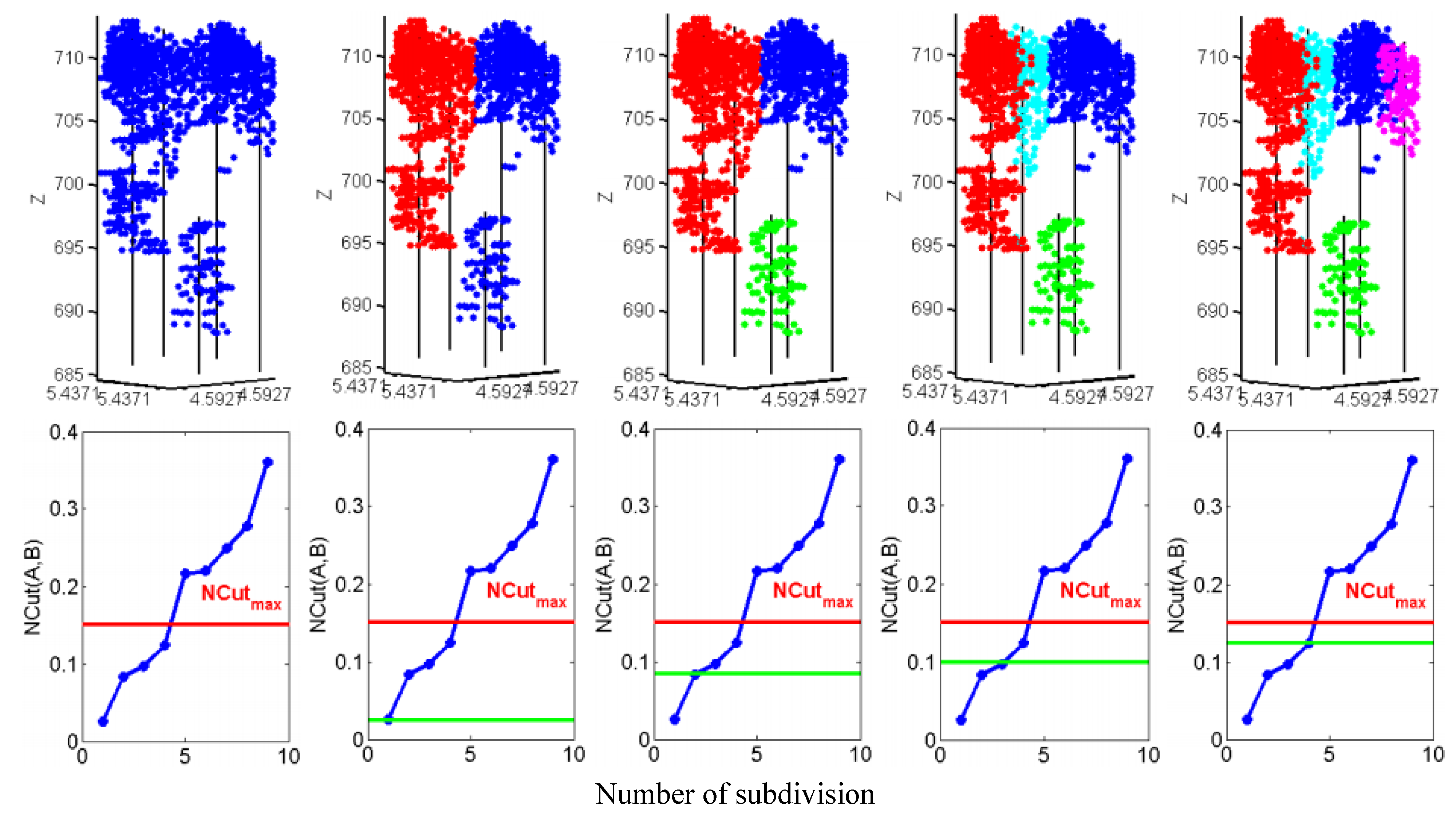
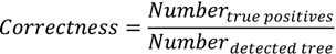
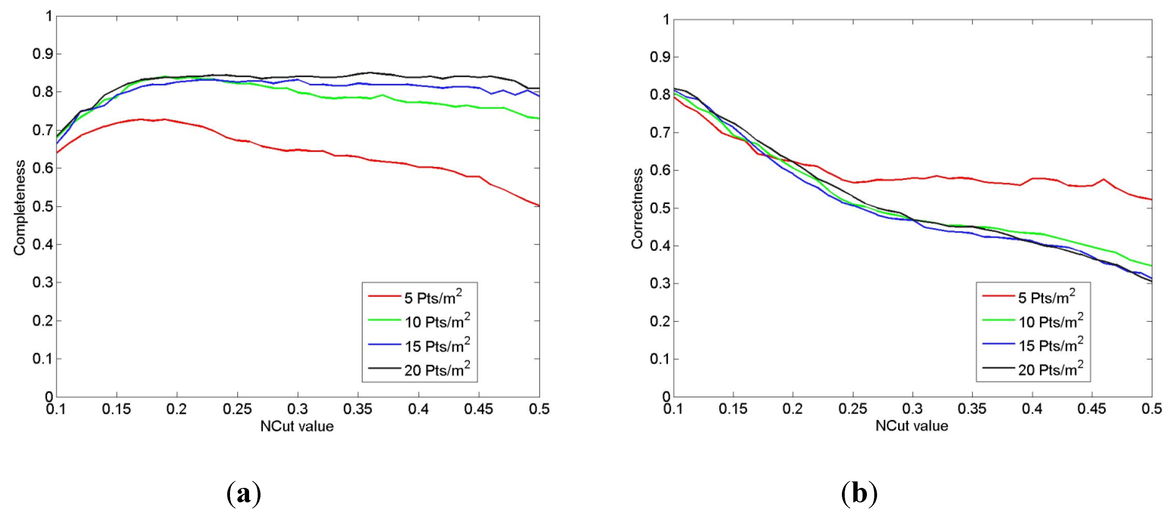
2.2.1. Threshold for Normalized Cut Value NCutThres
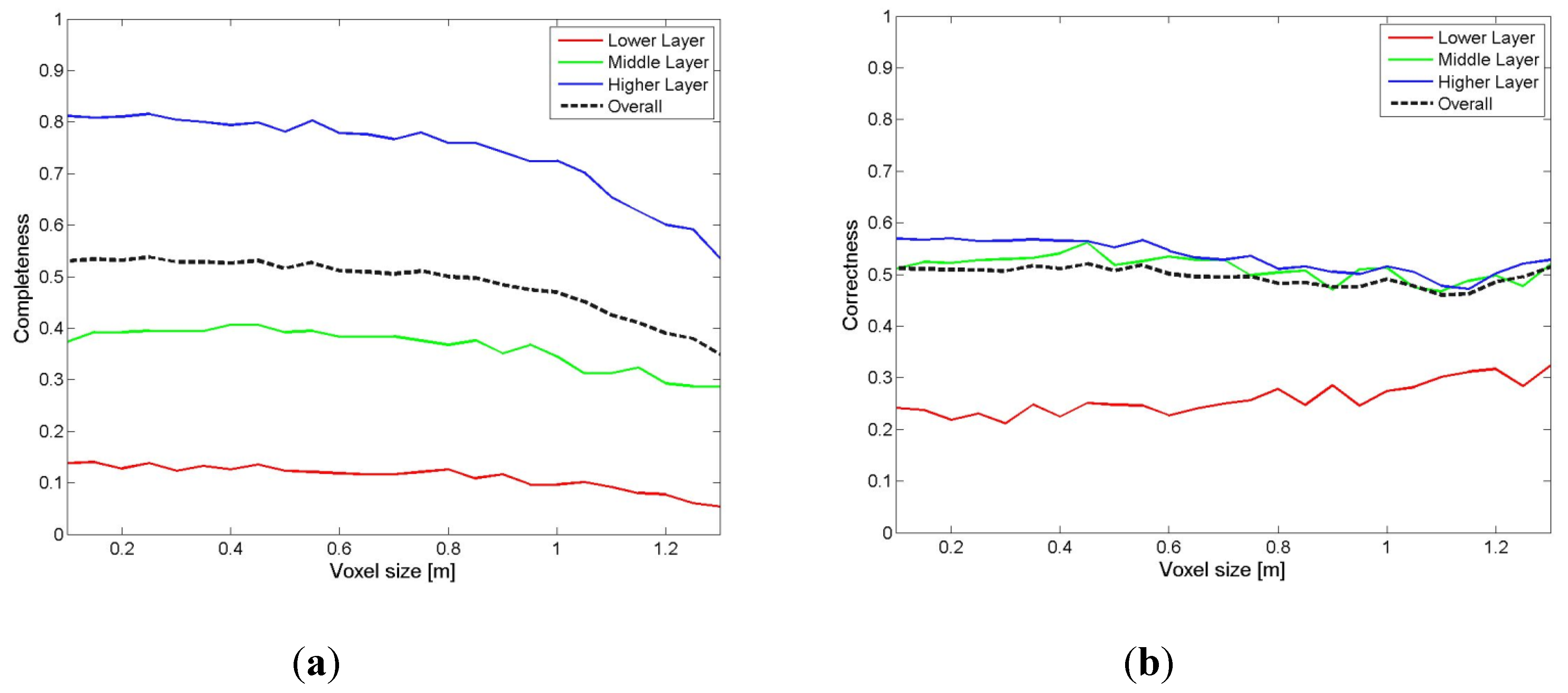
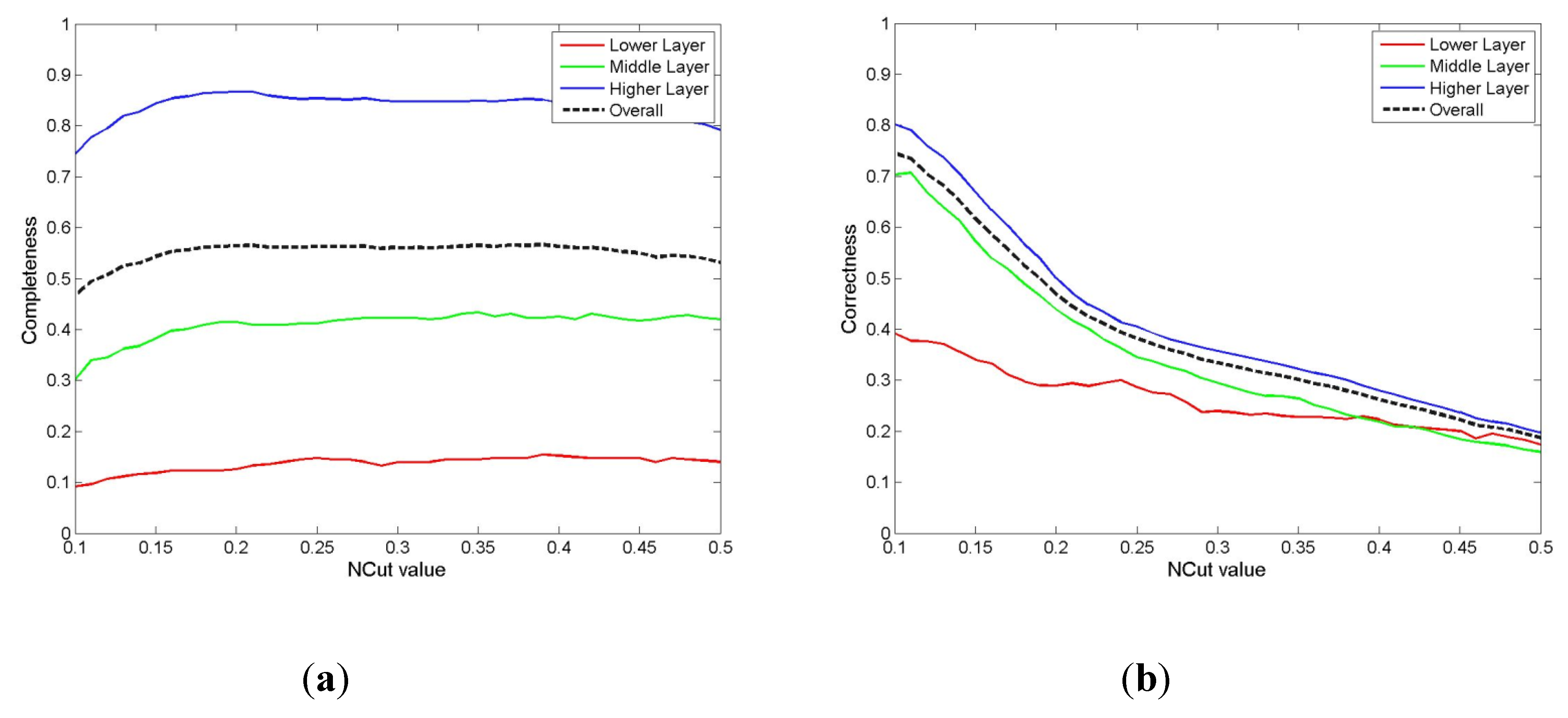
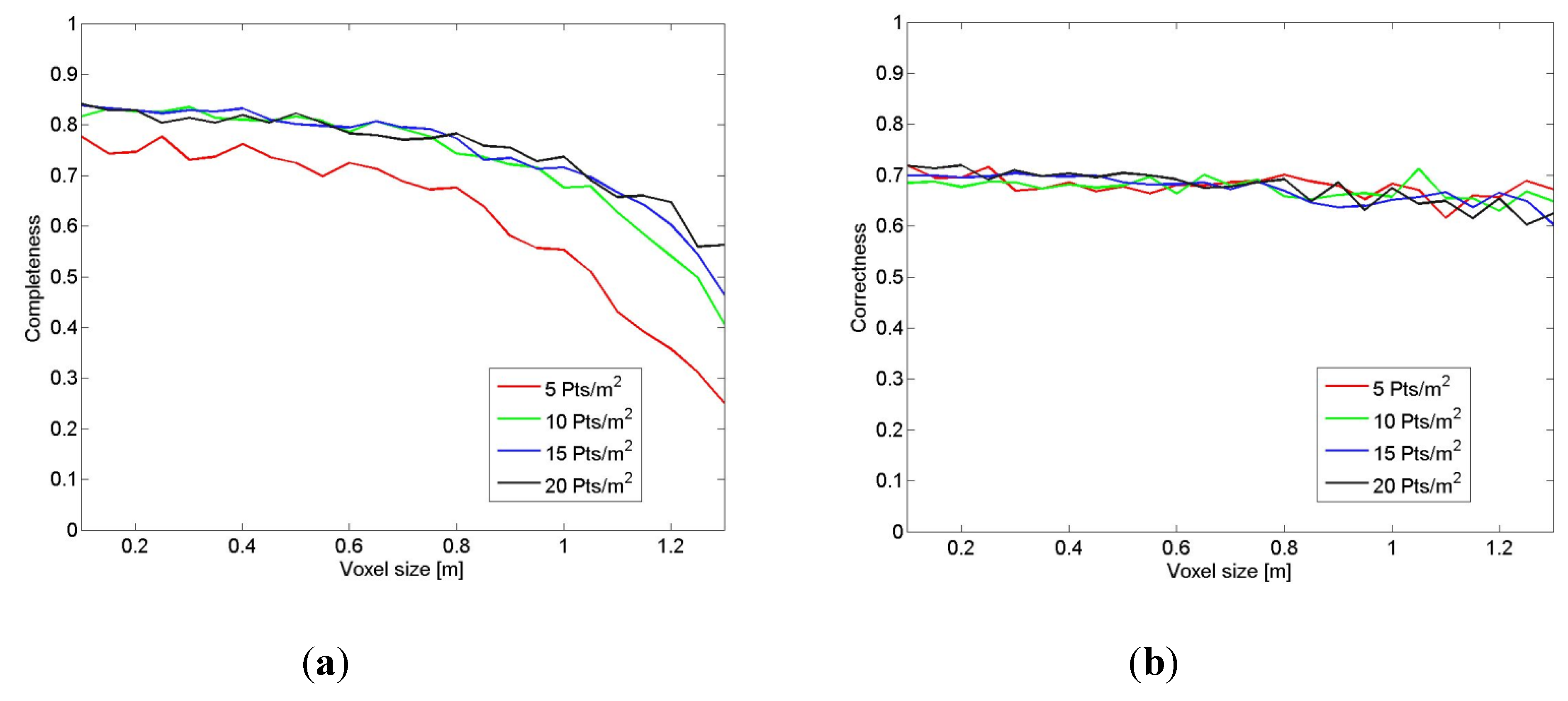
2.2.2. Voxel Size Vsize
 voxels (Figure 1a). Within each voxel of the size Vsize we collect N reflections
  , where only voxels comprising at least one reflection are used in the segmentation. The voxel structure is represented as a region adjacency graph G = {V,E} with V as the voxels representing the nodes and E as the edges formed between every pair of nodes. The similarity between two nodes {i,j}∈V is described by the weights wij which are computed from features associated with the voxels. Basically, the similarity between voxels decreases with increasing distance between two voxels and drops down to zero beyond the threshold rXY for the mutual distance in order to keep the graph G at a reasonable size for computation.
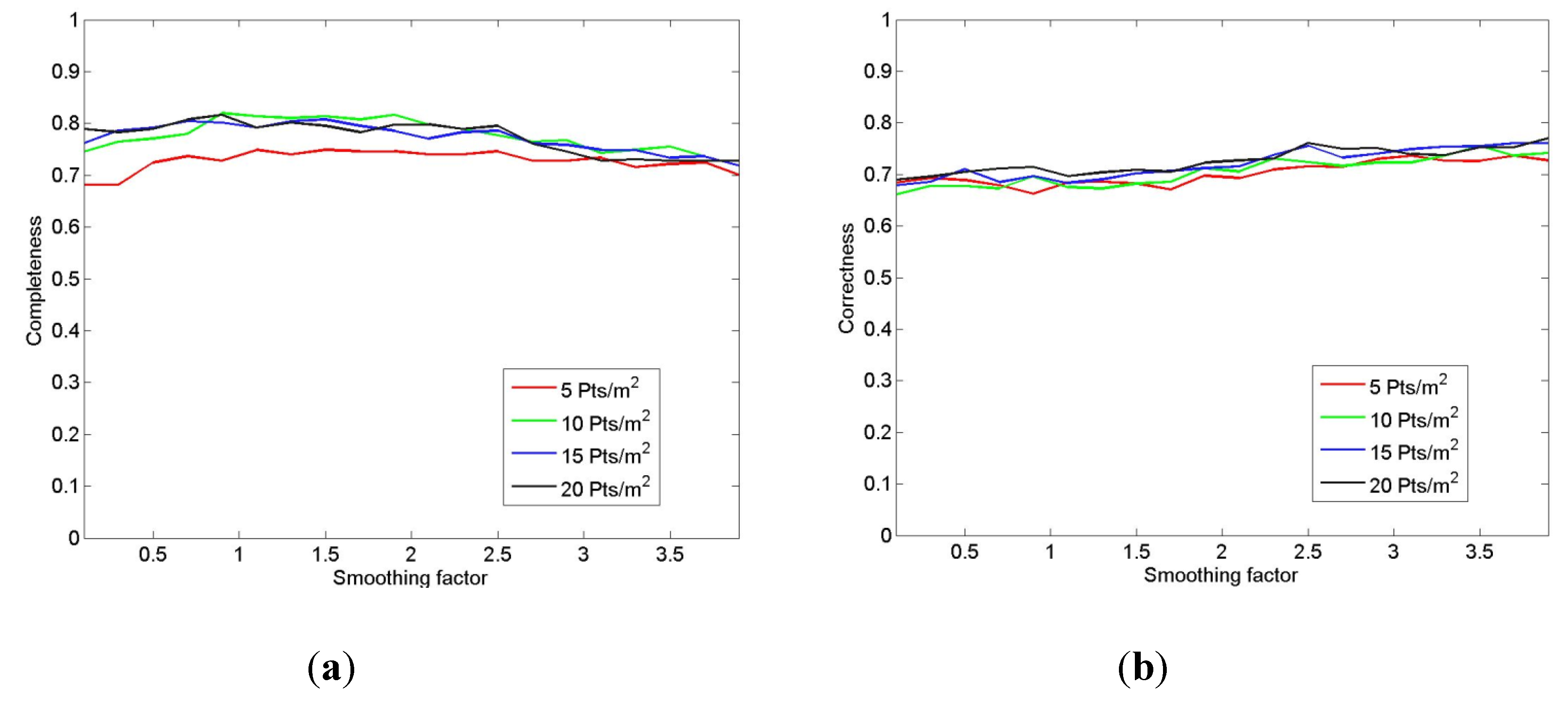
2.2.3. Smoothing Factor λ for CHM Generation.
3. Experiment
3.1. Material
3.1.1. Test Site I

| Plot | Size (ha) | Age (a) | Trees/ha | Deciduous (%) | N lower layer | N interm. layer | N upper layer |
|---|---|---|---|---|---|---|---|
| 21 | 0.20 | 160 | 500 | 66 | 37 | 14 | 48 |
| 22 | 0.20 | 160 | 540 | 79 | 19 | 60 | 29 |
| 55 | 0.15 | 240 | 830 | 5 | 77 | 21 | 20 |
| 56 | 0.23 | 170 | 340 | 10 | 31 | 19 | 27 |
| 57 | 0.10 | 100 | 450 | 0 | 0 | 4 | 41 |
| 58 | 0.10 | 85 | 440 | 14 | 10 | 4 | 30 |
| 59 | 0.10 | 40 | 2150 | 1 | 76 | 85 | 54 |
| 60 | 0.10 | 110 | 380 | 100 | 8 | 22 | 27 |
| 64 | 0.12 | 100 | 430 | 87 | 13 | 4 | 35 |
| 65 | 0.12 | 100 | 810 | 96 | 53 | 26 | 35 |
| 74 | 0.30 | 85 | 700 | 29 | 11 | 33 | 165 |
| 81 | 0.30 | 70 | 610 | 100 | 29 | 59 | 96 |
| 91 | 0.36 | 110 | 260 | 75 | 31 | 11 | 54 |
| 92 | 0.25 | 110 | 170 | 100 | 13 | 3 | 27 |
| 93 | 0.28 | 110 | 240 | 66 | 7 | 2 | 59 |
| 94 | 0.29 | 110 | 250 | 97 | 15 | 4 | 54 |
| 95 | 0.25 | 110 | 240 | 10 | 6 | 0 | 53 |
| 96 | 0.30 | 110 | 200 | 86 | 30 | 3 | 26 |
| Time of flight | May 2006 | May 2007 |
|---|---|---|
| Data set | I | II |
| Foliage | Leaf-off | Leaf-on |
| Scanner | Riegl LMS-Q560 | Riegl LMS-Q560 |
| Pts/m2 | 25 | 25 |
| Above ground level (AGL) (m) | 400 | 400 |
| Beam divergence (mrad) | ≤0.5 | ≤0.5 |
| Calibration parameter k | 1.902 | 1.736 |
3.1.2. Test Site II
| Plot | Size (ha) | Altitude (m) | Trees/ha | Deciduous (%) | N lower layer | N intern layer | N upper layer |
|---|---|---|---|---|---|---|---|
| 1 | 0.05 | 441 | 448 | 0 | 0 | 0 | 12 |
| 2 | 0.04 | 441 | 483 | 0 | 0 | 0 | 9 |
| 3 | 0.05 | 441 | 417 | 100 | 0 | 2 | 11 |
| 4 | 0.04 | 441 | 349 | 100 | 0 | 1 | 7 |
| 5 | 0.05 | 441 | 490 | 0 | 0 | 0 | 13 |
| 6 | 0.04 | 440 | 261 | 100 | 0 | 2 | 2 |
| 7 | 0.04 | 440 | 202 | 100 | 0 | 1 | 4 |
| 8 | 0.03 | 441 | 560 | 75 | 0 | 6 | 2 |
| 9 | 0.05 | 441 | 453 | 0 | 0 | 0 | 14 |
| 10 | 0.05 | 440 | 441 | 0 | 0 | 0 | 13 |
| 11 | 0.04 | 440 | 272 | 100 | 0 | 0 | 5 |
| 12 | 0.05 | 439 | 196 | 100 | 0 | 0 | 6 |
| 13 | 0.05 | 439 | 487 | 0 | 0 | 0 | 14 |
| 14 | 0.05 | 439 | 490 | 0 | 0 | 0 | 13 |
| 15 | 0.06 | 439 | 679 | 0 | 0 | 0 | 23 |
| 16 | 0.04 | 440 | 371 | 100 | 0 | 2 | 7 |
| 17 | 0.05 | 439 | 698 | 0 | 0 | 0 | 18 |
| 18 | 0.05 | 482 | 576 | 0 | 0 | 0 | 16 |
| 19 | 0.05 | 483 | 633 | 12 | 0 | 0 | 6 |
| 20 | 0.05 | 468 | 631 | 94 | 9 | 4 | 3 |
| 21 | 0.05 | 464 | 405 | 90 | 4 | 2 | 3 |
| 22 | 0.05 | 464 | 690 | 0 | 0 | 0 | 17 |
| 23 | 0.04 | 448 | 330 | 0 | 0 | 0 | 5 |
| 24 | 0.05 | 447 | 471 | 83 | 1 | 2 | 6 |
| 25 | 0.05 | 456 | 692 | 0 | 0 | 0 | 19 |
| 26 | 0.04 | 442 | 340 | 0 | 0 | 2 | 6 |
| 27 | 0.04 | 442 | 411 | 0 | 0 | 1 | 7 |
| Time of flight | March 2011 |
|---|---|
| Foliage | Leaf-off |
| Scanner | Riegl LMS-Q680i |
| Point density: Pts/m2 | 5, 10, 15, 20 |
| AGL (m) | 700 |
| Beam divergence (mrad) | <=0.5 |
| Scan angle | 0°–22.5° |
3.2. Field Data and Evaluation
3.2.1. Test Site I
| Time of acquisition | May 2006 | May 2007 | ||
|---|---|---|---|---|
| Tree height (m) | DBH (cm) | Tree height (m) | DBH (cm) | |
| Min | 5.10 | 7 | 5.10 | 7 |
| Max | 50.60 | 113 | 50.60 | 113 |
| Mean | 25.42 | 31.90 | 25.29 | 31.70 |
| Standard deviation | 10.70 | 17.90 | 10.68 | 17.60 |
3.2.2. Test Site II
| Time of acquisition | March 2011 | |
|---|---|---|
| Tree height (m) | DBH (cm) | |
| Min | 1.0 | 2.0 |
| Max | 44.0 | 50.0 |
| Mean | 21.2 | 22.8 |
| Standard deviation | 8.7 | 10.1 |
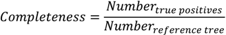
3.2.3. Evaluation
4. Results and Discussion
4.1. Results
4.1.1. Test Site I
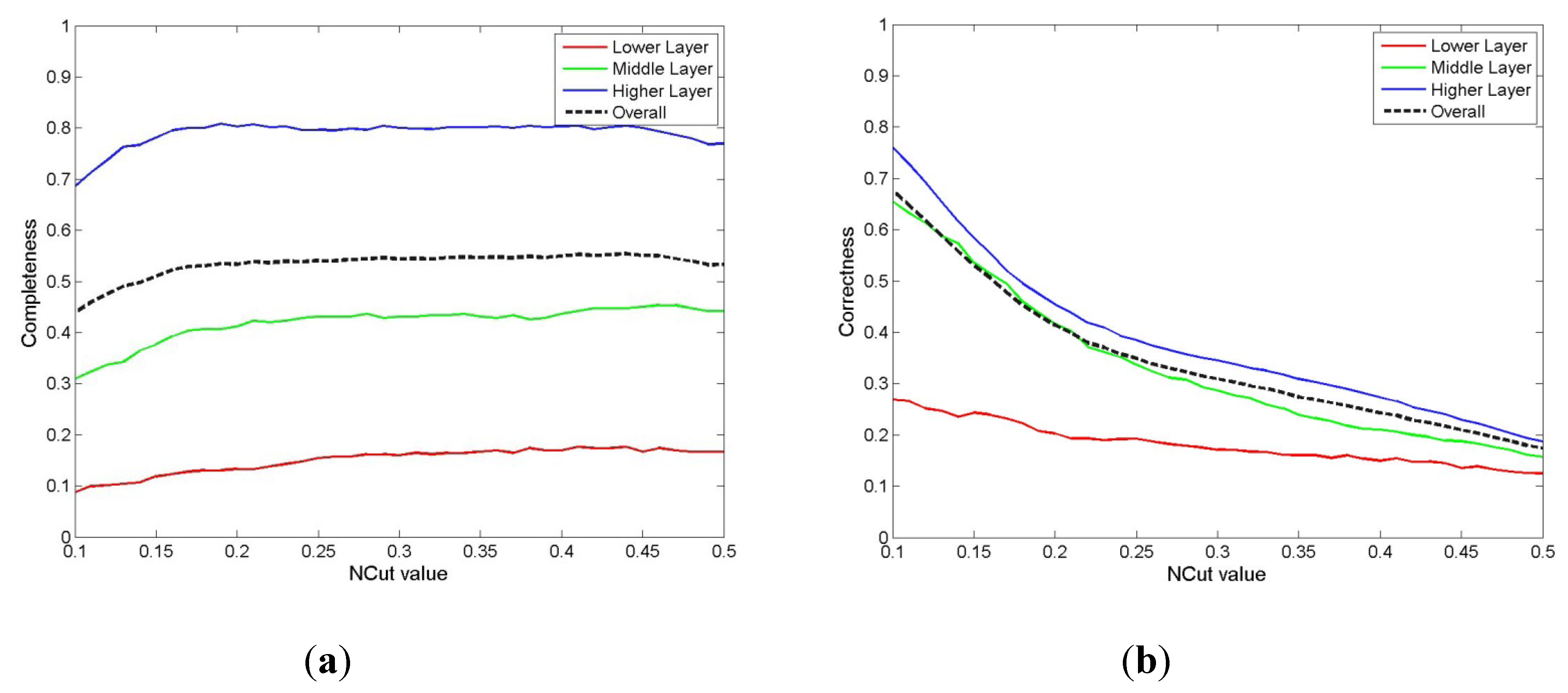


4.1.2. Test site II
4.2. Discussion
4.2.1. Test Site I vs. Test Site II
4.2.2. Foliage Condition
4.2.3. Point Density
5. Conclusions
Acknowledgments
Author Contributions
Conflicts of Interest
References
- Yao, W.; Stilla, U. Mutual enhancement of weak laser pulses for point cloud enrichment based on full-waveform analysis. Geosci. Remote Sens. 2010, 48, 3571–3579. [Google Scholar] [CrossRef]
- Vaughn, N.R.; Moskal, L.M.; Turnblom, E.C. Tree species detection accuracies using discrete point LiDAR and airborne waveform LiDAR. Remote Sens. 2012, 4, 377–403. [Google Scholar] [CrossRef]
- Yao, W.; Krzystek, P.; Heurich, M. Tree species classification and estimation of stem volume and DBH based on single tree extraction by exploiting airborne full-waveform LiDAR data. Remote Sens. Environ. 2012, 123, 368–380. [Google Scholar] [CrossRef]
- Stilla, U.; Yao, W.; Jutzi, B. Detection of weak laser pulses by full waveform stacking. In PIA07 Photogrammetric Image Analysis 2007; International Archives of Photogrammetry, Remote Sensing, and Spatial Information Sciences; Stilla, U., Ed.; Volume 36, (3/W49A); pp. 25–30.
- Reitberger, J.; Krzystek, P.; Stilla, U. Analysis of full waveform LiDAR data for the classification of deciduous and coniferous trees. Int. J. Remote Sens. 2008, 29, 1407–1431. [Google Scholar] [CrossRef]
- Næsset, E. Predicting forest stand characteristics with airborne scanning laser using a practical two-stage procedure and field data. Remote Sens. Environ. 2002, 80, 88–99. [Google Scholar] [CrossRef]
- White, J.C.; Wulder, M.A.; Vastaranta, M.; Coops, N.C.; Pitt, D.; Woods, M. The utility of image-based point clouds for forest inventory: A comparison with airborne laser scanning. Forests 2013, 4, 518–536. [Google Scholar] [CrossRef]
- He, Q.; Chen, E.; An, R.; Li, Y. Above-ground biomass and biomass components estimation using LiDAR data in a coniferous forest. Forests 2013, 4, 984–1002. [Google Scholar] [CrossRef]
- Andersen, H.E.; McGaughey, R.J.; Reutebuch, S.E. Estimating forest canopy fuel parameters using LiDAR data. Remote Sens. Environ. 2005, 94, 441–449. [Google Scholar] [CrossRef]
- Nelson, R.; Krabill, W.; Tonelli, J. Estimating forest biomass and volume using airborne laser data. Remote Sens. Environ. 1988, 24, 247–267. [Google Scholar] [CrossRef]
- Heurich, M.; Thoma, F. Estimation of forestry stand parameters using laser scanning data in temperate, structurally rich natural beech (Fagus sylvatica) and spruce (Picea abies) forests. Forestry 2008, 81, 645–661. [Google Scholar] [CrossRef]
- Kantola, T.; Vastaranta, M.; Lyytikäinen-Saarenmaa, P.; Holopainen, M.; Kankare, V.; Talvitie, M.; Hyyppä, J. Classification of needle loss of individual Scots pine trees by means of airborne laser scanning. Forests 2013, 4, 386–403. [Google Scholar] [CrossRef]
- Ene, L.; Næsset, E.; Gobakken, T. Single tree detection in heterogeneous boreal forests using airborne laser scanning and area-based stem number estimates. Int. J. Remote Sens. 2012, 33, 5171–5193. [Google Scholar] [CrossRef]
- Persson, A.; Holmgren, J.; Soderman, U. Detecting and measuring individual trees using an airborne laser scanner. Photogramm. Eng. Remote Sens. 2002, 68, 925–932. [Google Scholar]
- Yu, X.; Hyyppä, J.; Vastaranta, M.; Holopainen, M.; Viitala, R. Predicting individual tree attributes from airborne laser point clouds based on the random forests technique. ISPRS J. Photogramm. Remote Sens. 2011, 64, 28–37. [Google Scholar]
- Reitberger, J.; Schnörr, C.; Krzystek, P.; Stilla, U. 3D segmentation of single trees exploiting full waveform LiDAR data. ISPRS J. Photogramm. Remote Sens. 2009, 64, 561–574. [Google Scholar] [CrossRef]
- Vauhkonen, J.; Ene, L.; Gupta, S.; Heinzel, J.; Holmgren, J.; Pitkänen, J.; Solberg, S.; Wang, Y.; Weinacker, H.; Hauglin, K.M.; Lien, V.; Packalén, P.; Gobakken, T.; Koch, B.; Næsset, E.; Tokola, T.; Maltamo, M. Comparative testing of single tree detection algorithms under different types of forest. Forestry 2012, 3, 27–40. [Google Scholar]
- Abed, F.M.; Mills, J.P.; Miller, P.E. Echo amplitude normalization of full-waveform airborne laser scanning data based on robust incidence angle estimation. IEEE Trans. Geosci. Remote Sens. 2012, 50, 2910–2918. [Google Scholar] [CrossRef]
- Korpela, I.; Ørka, H.O.; Maltamo, M.; Tokola, T.; Hyyppä, J. Tree species classification using airborne LiDAR-effects of stand and tree parameters, downsizing of training set, intensity normalization, and sensor type. Silva Fenn. 2010, 44, 319–339. [Google Scholar]
- Kaartinen, H.; Hyyppä, J.; Yu, X.; Vastaranta, M.; Hyyppä, H.; Kukko, A.; Holopainen, M.; Heipke, C.; Hirschmugl, M.; Morsdorf, F.; Næsset, E.; Pitkänen, J.; Popescu, S.; Solberg, S.; Wolf, B.M.; Wu, J.C. An international comparison of individual tree detection and extraction using airborne laser scanning. Remote Sens. 2012, 4, 950–974. [Google Scholar] [CrossRef] [Green Version]
- Gonzalez, P.; Asner, G.P.; Battles, J.; Lefsky, M.A.; Waring, K.M.; Palace, M. Forest carbon densities and uncertainties from LiDAR, quickbird, and field measurements in California. Remote Sens. Environ. 2011, 114, 1561–1575. [Google Scholar]
- Lu, D.; Chen, Q.; Wang, G.; Moran, E.; Batistella, M.; Zhang, M.; Laurin, G.V.; Saah, D. Aboveground forest biomass estimation with landsat and LiDAR data and uncertainty analysis of the estimates. Int. J. For. Res. 2012. [Google Scholar] [CrossRef]
- Monnet, J.M.; Merminy, E.; Chanussotz, J.; Berger, F. Tree top detection using local maxima filtering: a parameter sensitivity analysis. In Proceedings of the 10th International Conference on LiDAR Applications for Assessing Forest Ecosystems (Silvilaser 2010), Freiburg, Germany, September 2010; pp. 14–17.
- Palleja, T.; Tresanchez, M.; Teixido, M.; Sanz, R.; Rosell, J.R.; Palacin, J. Sensitivity of tree volume measurement to trajectory errors from a terrestrial LiDAR scanner. Agric. For. Meteorol. 2010, 150, 1420–1427. [Google Scholar] [CrossRef]
- Mutlu, M.; Popescu, S.C.; Zhao, K. Sensitivity analysis of fire behavior modeling with LiDAR derived surface fuel maps. For. Ecol. Manag. 2008, 256, 289–294. [Google Scholar] [CrossRef]
- D’Errico, J. 2006, Surface fitting using gridfit. Available online: http://www.mathworks.com/matlabcentral/fileexchange (accessed on 1 October 2009).
- Shi, J.; Malik, J. Normalized cuts and image segmentation. Pattern Anal. Mach. Intell. 2000, 22, 888–905. [Google Scholar] [CrossRef]
- Reitberger, J. 3D-Segmentierung von Einzelbäumen und Baumartenklassifikation aus Daten flugzeuggetragener Full Waveform Laserscanner. Ph.D. Thesis, Technische Universitaet Muenchen, München, Germany, 2010. [Google Scholar]
- Heurich, M. Automatic recognition and measurement of single trees based on data from airborne laser scanning over the richly structured natural forests of the Bavarian Forest National Park. For. Ecol. Manag. 2008, 255, 2416–2433. [Google Scholar] [CrossRef]
- Jakubowski, M.K.; Guo, Q.; Kelly, M. Tradeoffs between LiDAR pulse density and forest measurement accuracy. Remote Sens. Environ. 2013, 130, 245–253. [Google Scholar] [CrossRef]
© 2014 by the authors; licensee MDPI, Basel, Switzerland. This article is an open access article distributed under the terms and conditions of the Creative Commons Attribution license (http://creativecommons.org/licenses/by/3.0/).
Share and Cite
Yao, W.; Krull, J.; Krzystek, P.; Heurich, M. Sensitivity Analysis of 3D Individual Tree Detection from LiDAR Point Clouds of Temperate Forests. Forests 2014, 5, 1122-1142. https://doi.org/10.3390/f5061122
Yao W, Krull J, Krzystek P, Heurich M. Sensitivity Analysis of 3D Individual Tree Detection from LiDAR Point Clouds of Temperate Forests. Forests. 2014; 5(6):1122-1142. https://doi.org/10.3390/f5061122
Chicago/Turabian StyleYao, Wei, Jan Krull, Peter Krzystek, and Marco Heurich. 2014. "Sensitivity Analysis of 3D Individual Tree Detection from LiDAR Point Clouds of Temperate Forests" Forests 5, no. 6: 1122-1142. https://doi.org/10.3390/f5061122