Evaluating an Automated Approach for Monitoring Forest Disturbances in the Pacific Northwest from Logging, Fire and Insect Outbreaks with Landsat Time Series Data


Abstract
:
1. Introduction
- Are long-term productivity declines in Pacific Northwest forests observed with GIMMS “g” AVHRR NDVI an error or real?
- Can an image classification algorithm be used on annual anniversary LTSS with common spectral indices to extract forest disturbance type? If so, what is the change map accuracy with uncertainty?
- What were the dominant agents of disturbance at the coarse scale of AVHRR observations?
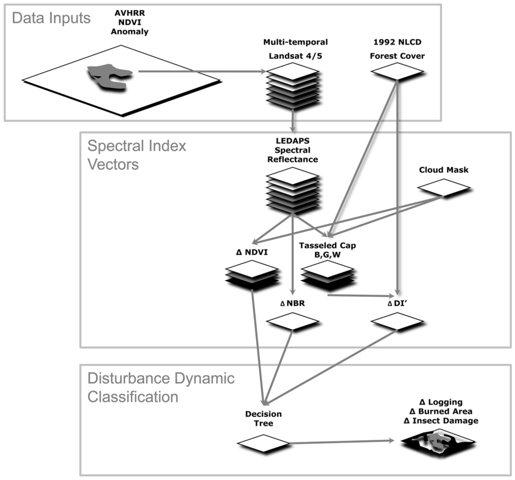
2. Data and Methods
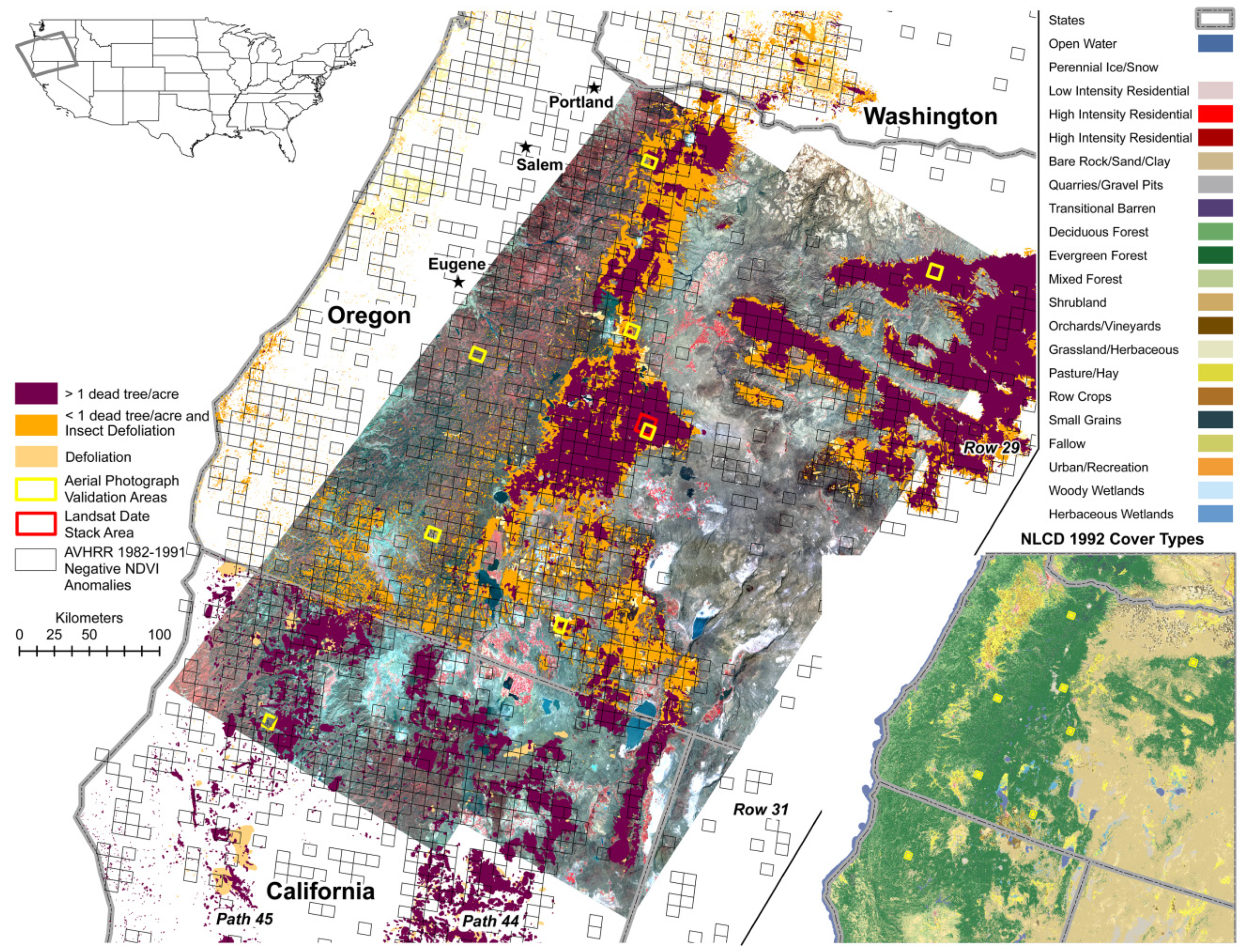
2.1. Study Area

2.2. AVHRR Data
2.3. Landsat Data

| Path Row | 044029 | 044030 | 044031 | 045029 | 045030 | 045031 |
|---|---|---|---|---|---|---|
| Date | 5 July 1984 | 5 July 1984 | 5 July 1984 | ∙∙∙ | ∙∙∙ | ∙∙∙ |
| ∙∙∙ | 9 Aug. 1985 | 25 Aug. 1985 | 16 Aug. 1985 | 16 Aug. 1985 | 16 Aug. 1985 | |
| 12 Aug. 1986 | 12 Aug. 1986 | 12 Aug. 1986 | 19 Aug. 1986 | 19 Aug. 1986 | 16 Aug. 1986 | |
| 16 Sep. 1987 | 31 Aug. 1987 | 15 Aug. 1987 | 7 Sep. 1987 | 7 Sep. 1987 | 6 Aug. 1987 | |
| 2 Sep. 1988 | 1 Aug. 1988 | 1 Aug. 1988 | 9 Sep. 1988 | 24 Aug. 1988 | 24 Aug. 1988 | |
| 21 Sep. 1989 | 4 Aug. 1989 | 4 Aug. 1989 | 12 Sep. 1989 | 12 Sep. 1989 | 11 Aug. 1989 | |
| 8 Sep. 1990 | 8 Sep. 1990 | 8 Sep. 1990 | 14 Aug. 1990 | 30 Aug. 1990 | 30 Aug. 1990 | |
| 26 Aug. 1991 | 10 Aug. 1991 | 10 Aug. 1991 | 17 Aug. 1991 | 2 Sep. 1991 | 2 Sep. 1991 | |
| 28 Aug. 1992 | 28 Aug. 1992 | ∙∙∙ | 3 Aug. 1992 | 3 Aug. 1992 | 19 Aug. 1992 | |
| 31 Aug. 1993 | 31 Aug. 1993 | 31 Aug. 1993 | ∙∙∙ | 7 Sep. 1993 | ∙∙∙ | |
| 19 Sep. 1994 | 18 Aug. 1994 | 18 Aug. 1994 | 9 Aug. 1994 | 9 Aug. 1994 | 9 Aug. 1994 | |
| 21 Aug. 1995 | 5 Aug. 1995 | 5 Aug. 1995 | 13 Sep. 1995 | 13 Sep. 1995 | 12 Aug. 1995 |
2.3.1. Landsat Index Generation
2.3.2. Landsat Forest Mask
2.3.3. Cloud Masking
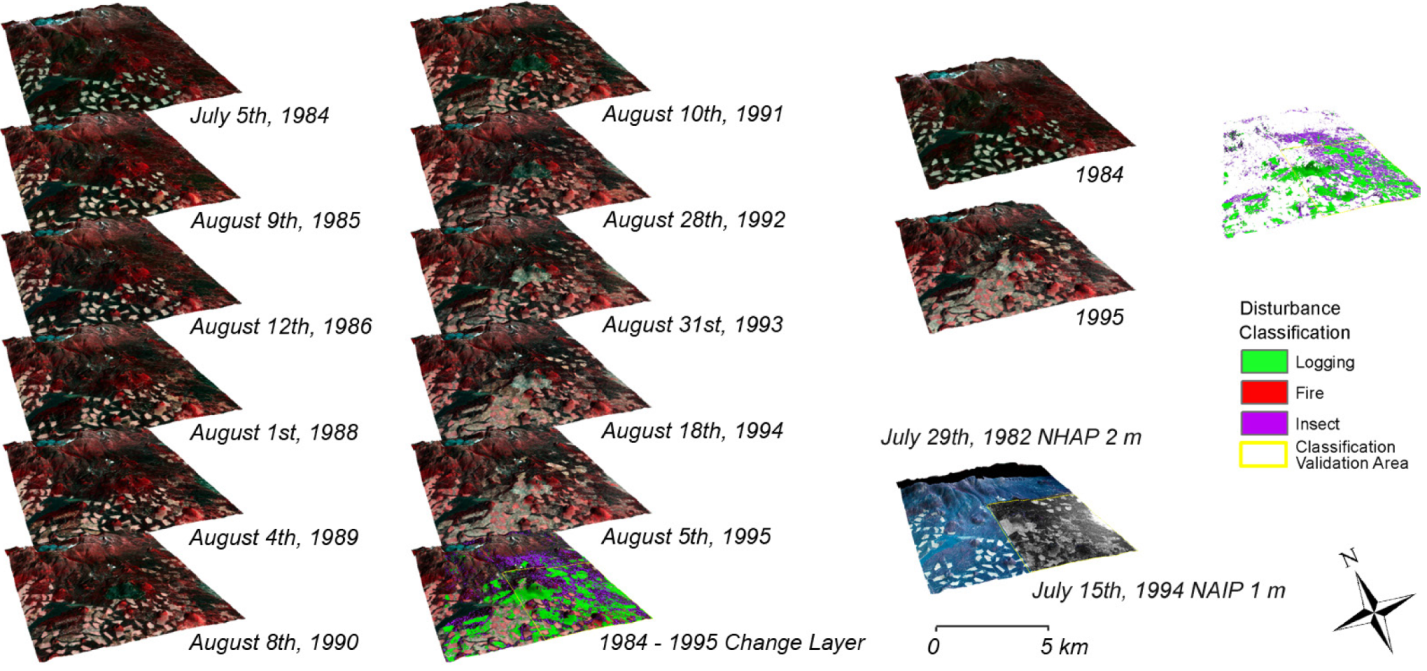
2.4. Landsat Disturbance Classification

Running Landsat Classifications
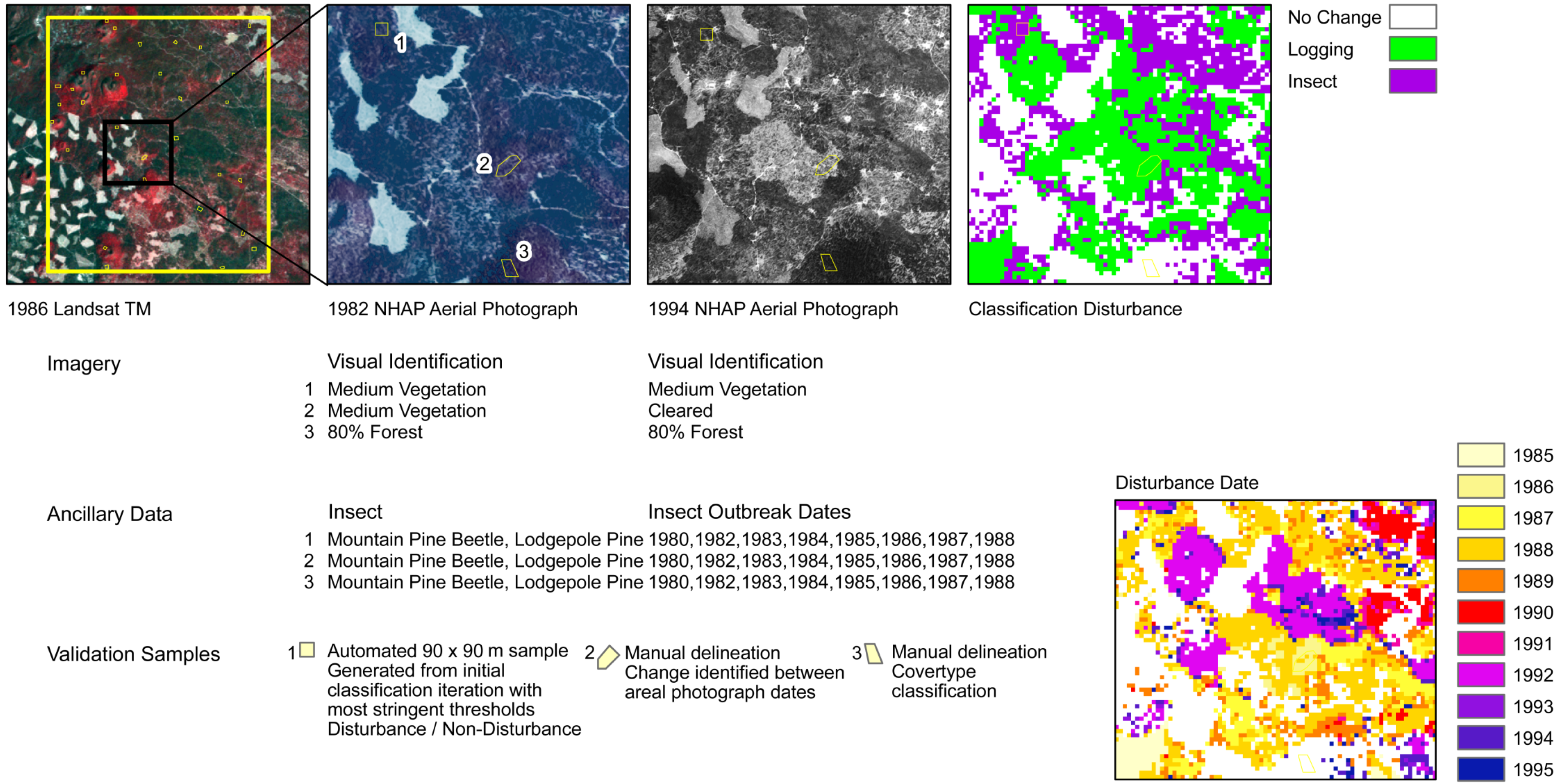
2.5. Independent Classification Evaluation Data
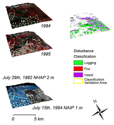
2.5.1. Multi-Temporal High Resolution Air Photos
2.5.2. Monitoring Trends in Burn Severity Data
2.5.3. Aerial Detection Survey Data
| Landsat Path Row | Lat. | Lon. | Air Photo ID | Date | Spatial Resolution | Spectral Resolution | Ortho* |
|---|---|---|---|---|---|---|---|
| 044029 | 45.1 | −119.3 | NC1NHAP810117221 | 15 Aug. 1981 | 2 m | CIR | Y |
| NP0NAPP001224139 | 9 Sep. 1989 | 1 m | B/W Pan | Y | |||
| N10NAPPW07098135 | 29 June 1994 | 1 m | B/W Pan | Y | |||
| 044030 | 43.6 | −121.2 | NC1NHAP820065108 | 29 July 1982 | 2 m | CIR | N |
| N10NAPPW07115152 | 20 July 1994 | 1 m | B/W Pan | N | |||
| N10NAPPW07115152 | 20 July 1994 | 1 m | B/W Pan | N | |||
| 044031 | 42.3 | −121.3 | NC1NHAP820065153 | 29 July 1982 | 2 m | CIR | Y |
| N10NAPPW07109231 | 14 July 1994 | 1 m | B/W Pan | Y | |||
| 045029 | 44.2 | −121.6 | NC1NHAP820093044 | 27 Aug. 1982 | 2 m | CIR | N |
| N10NAPPW07099156 | 29 June 1994 | 1 m | B/W Pan | N | |||
| 45.2 | −121.9 | NC1NHAP810113089 | 9 Aug/ 1981 | 2 m | CIR | N | |
| 045030 | 42.6 | −122.6 | NC1NHAP820079166 | 17 Aug. 1982 | 2 m | CIR | Y |
| N10NAPPW07180105 | 29 June 1994 | 1 m | B/W Pan | Y | |||
| 43.7 | −122.7 | NC1NHAP820055148 | 23 July 1982 | 2 m | CIR | Y | |
| N10NAPPW07180241 | 29 June 1994 | 1 m | B/W Pan | Y | |||
| 045031 | 41.2 | −123.1 | NC1NHAP830465142 | 9 Sep. 1983 | 2 m | CIR | Y |
| N10NAPPW06257137 | 24 Aug 1994 | 1 m | B/W Pan | Y |
2.5.4. Good Practice Classification Accuracy Assessment

2.5.5. Automated Classification Evaluation
2.5.6. Manual Classification Evaluation and Statistical Analysis
3. Results
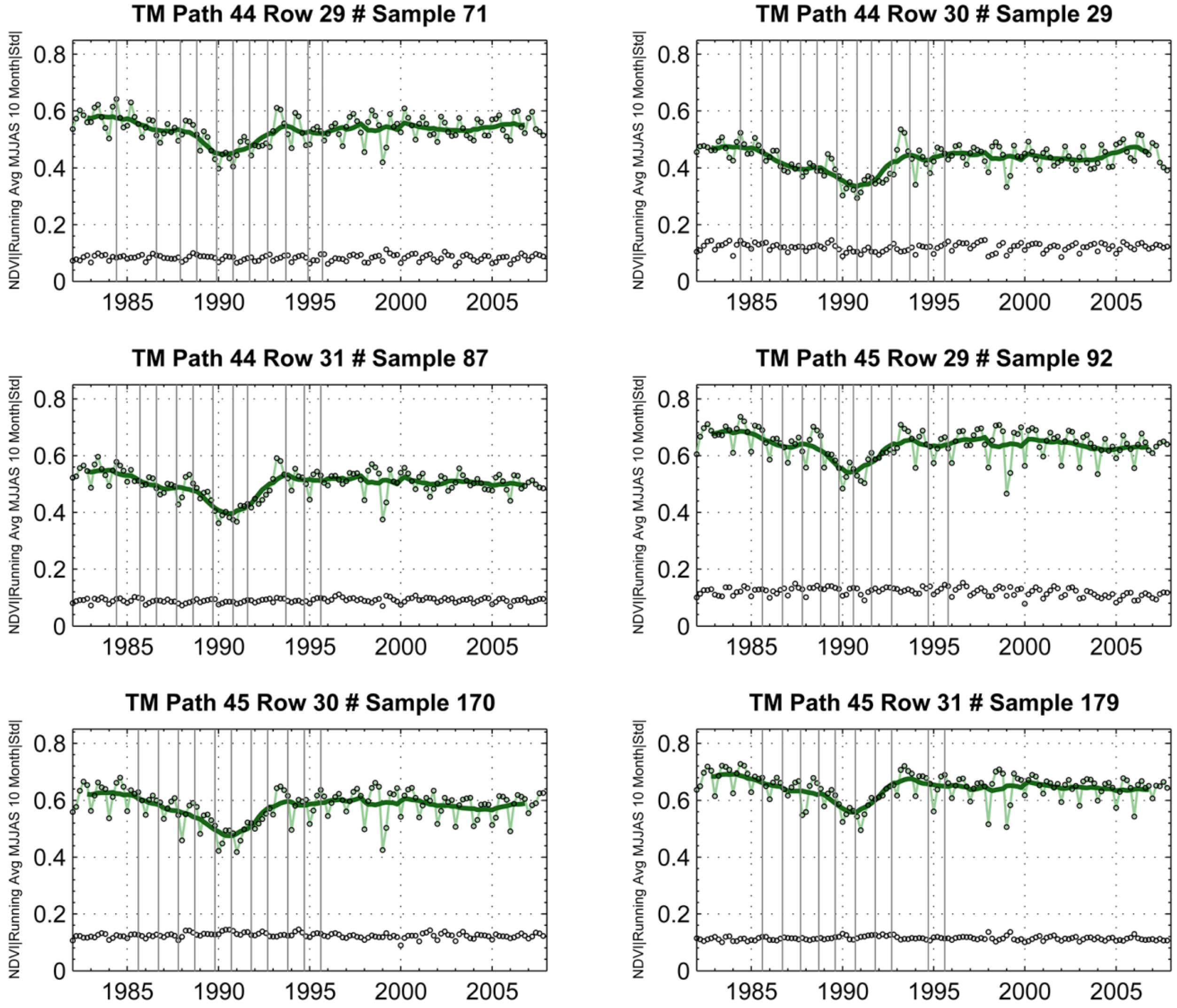
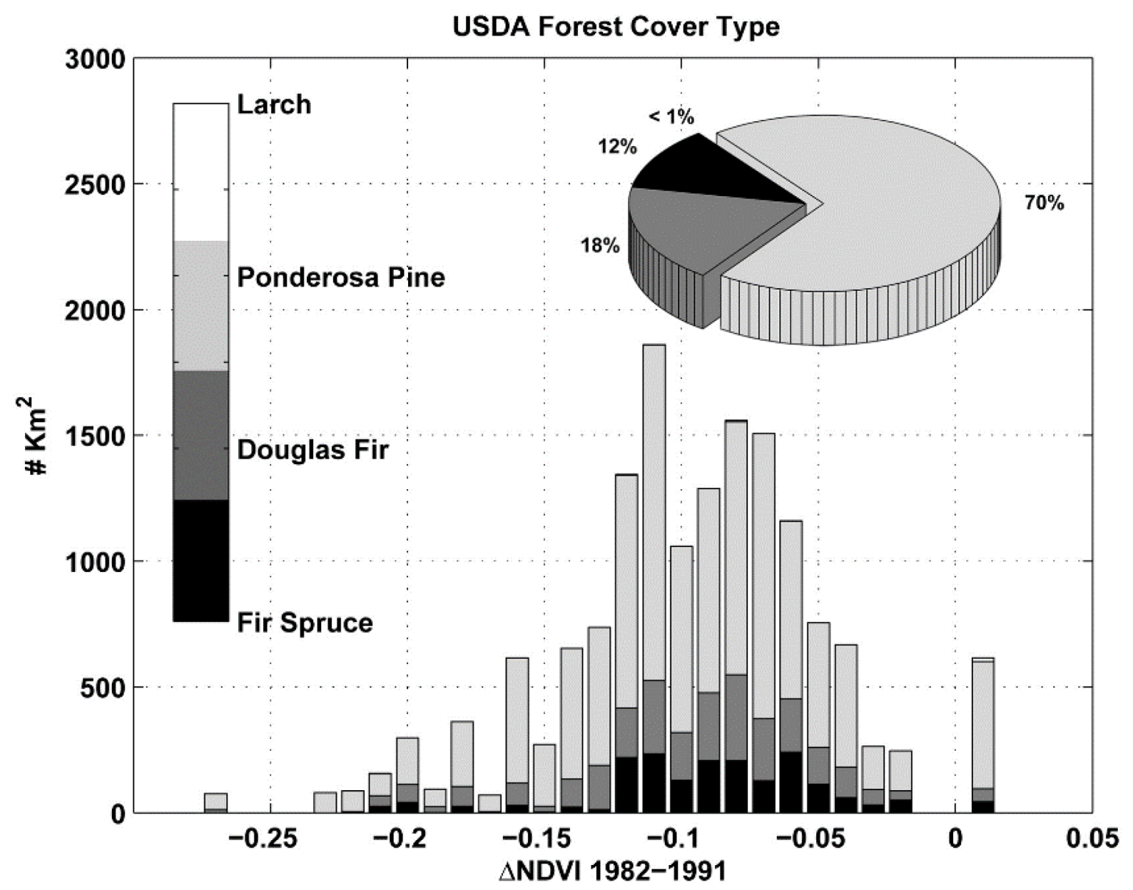
3.1. Drivers of AVHRR NDVI Declines


3.2. Ensemble Accuracy Assessment Error Matrices
| Reference | ||||||||||
|---|---|---|---|---|---|---|---|---|---|---|
| Stable Forest | Logging | Fire | Insect | Total | User’s | Producer’s | Overall | Map Area (ha) | ||
| Map | Stable forest | 0.74 | 0.03 | 0.02 | 0.03 | 0.82 | 0.90 ± 0.02 | 0.95 ± 0.01 | 0.87 ± 0.02 | 5,046,744 |
| Logging | 0.03 | 0.11 | 0.01 | 0.00 | 0.14 | 0.74 ± 0.03 | 0.76 ± 0.03 | 880,224 | ||
| Fire | 0.00 | 0.00 | 0.01 | 0.00 | 0.01 | 1.00 ± 0.00 | 0.23 ± 0.07 | 41,949 | ||
| Insect | 0.01 | 0.00 | 0.00 | 0.01 | 0.02 | 0.38 ± 0.05 | 0.21 ± 0.06 | 151,096 | ||
| Total | 0.79 | 0.14 | 0.03 | 0.04 | 1 | 6,120,013 | ||||

3.3. Index Performance by Disturbance Type and Cover Type


3.4. Spatial Disturbance Type Trends
4. Discussion
5. Conclusions
Acknowledgments
Author Contributions
Conflicts of Interest
References
- Gower, S.T. Patterns and Mechanisms of the Forest Carbon Cycle. Ann. Rev. Environ. Resour. 2003, 28, 169–204. [Google Scholar] [CrossRef]
- Schimel, D.; Braswell, B. Continental scale variability in ecosystem processes: Models, data, and the role of disturbance. Ecol. Monogr. 1997, 67, 251–271. [Google Scholar] [CrossRef]
- Thorton, P.E.; Clark, K.L.; Falge, E.; Ellsworth, D.S.; Goldstein, A.H.; Monson, R.K.; Hollinger, D.; Falk, M.; Chen, J.; Sparks, J.P.; et al. Modeling and measuring the effects of disturbance history and climate on carbon and watrer budgets in evergreen needleleaf forests. Agric. For. Meterol. 2002, 113, 185–222. [Google Scholar] [CrossRef]
- Houghton, R.A. Revised estimates of the annual net flux of carbon to the atmosphere from changes in land use and land management 1850–2000. Tellus 2003, 55B, 378–390. [Google Scholar] [CrossRef]
- Houghton, R.A.; Hackler, J.L.; Lawrence, K.T. The U.S. carbon budget: Contributions from land-use change. Science 1999, 285, 574–578. [Google Scholar] [CrossRef] [PubMed]
- Pacala, S.W.; Hurtt, G.C.; Baker, D.; Peylin, P.; Houghton, R.A.; Birdsey, R.A.; Heath, L.; Sundquist, E.T.; Stallard, R.F.; Ciais, P.; et al. Consistent Land- and Atmosphere-Based U.S. Carbon Sink Estimates. Science 2001, 292, 2316–2320. [Google Scholar] [CrossRef] [PubMed]
- Pan, Y.D.; Birdsey, R.A.; Fang, J.Y.; Houghton, R.; Kauppi, P.E.; Kurz, W.A.; Phillips, O.L.; Shvidenko, A.; Lewis, S.L.; Canadell, J.G.; et al. A Large and Persistent Carbon Sink in the World’s Forests. Science 2011, 333, 988–993. [Google Scholar] [CrossRef] [PubMed]
- Caspersen, J.P.; Pacala, S.W.; Jenkins, J.C.; Hurtt, G.C.; Moorcroft, P.R.; Birdsey, R.A. Contributions of Land-Use History to Carbon Accumulation in U.S. Forests. Science 2000, 290, 1148–1151. [Google Scholar] [CrossRef] [PubMed]
- King, A.W. The First State of the Carbon Cycle Report (SOCCR): The North American Carbon Budget and Implications for the Global Carbon Cycle; King, A.W., Dilling, L., Zimmerman, G.P., Fairman, D.M., Houghton, R.A., Marland, G.H., Rose, A.Z., Wilbanks, T.J., Eds.; U.S. Climate Change Science Program and the Subcommittee on Global Change Research, US Government: Oak Ridge, Tennese, USA, 2007; Volume 2.2, p. 446.
- Irvine, J.; Law, B.E.; Hibbard, K.A. Postfire carbon pools and fluxes in semiarid ponderosa pine in Central Oregon. Glob. Chang. Biol. 2007, 13, 1748–1760. [Google Scholar] [CrossRef]
- Kurz, W.A.; Dymond, C.C.; Stinson, G.; Rampley, G.J.; Neilson, E.T.; Carroll, A.L.; Ebata, T.; Safranyik, L. Mountain pine beetle and forest carbon feedback to climate change. Nature 2008, 452, 987–990. [Google Scholar] [CrossRef] [PubMed]
- Tucker, C.J.; Pinzon, J.E.; Brown, M.E.; Slayback, D.A.; Pak, E.W.; Mahoney, R.; Vermote, E.F.; Saleous, N.E. An Extended AVHRR 8-km NDVI Data Set Compatible with MODIS and SPOT Vegetation NDVI Data. Int. J. Remote Sens. 2005, 26, 4485–4498. [Google Scholar] [CrossRef]
- Busing, R.T.; Solomon, A.M.; McKane, R.B.; Burdick, C.A. Forest dynamics in Oregon landscapes: Evaluation and application of an individual-based model. Ecol. Appl. 2007, 17, 1967–1981. [Google Scholar] [CrossRef] [PubMed]
- Filip, G.M.; Maffei, H.; Chadwick, K.L. Forest health decline in a central Oregon mixed-conifer forest revisited after wildfire: A 25-year case study. West. J. Appl. For. 2007, 22, 278–284. [Google Scholar]
- Turner, D.P.; Koerper, G.J.; Harmon, M.E.; Lee, J.J. A Carbon Budget for Forests of the Conterminous United-States. Ecol. Appl. 1995, 5, 421–436. [Google Scholar] [CrossRef]
- Potter, C.; Klooster, S.; Hiatt, S.; Fladeland, M.; Genovese, V.; Gross, P. Satellite-derived estimates of potential carbon sequestration through afforestation of agriculture lands in the United States. Clim. Chang. 2007, 80, 323–336. [Google Scholar] [CrossRef]
- Coops, N.C.; Waring, R.H. Estimating forest productivity in the eastern Siskiyou Mountains of southwestern Oregon using a satellite driven process model, 3-PGS. Can. J. For. Res. Rev. Can. Rech. For. 2001, 31, 143–154. [Google Scholar] [CrossRef]
- Kennedy, R.E.; Turner, D.P.; Cohen, W.B.; Guzy, M. A method to efficiently apply a biogeochemical model to a landscape. Landsc. Ecol. 2006, 21, 213–224. [Google Scholar] [CrossRef]
- Law, B.E.; Turner, D.; Campbell, J.; Sun, O.J.; van Tuyl, S.; Ritts, W.D.; Cohen, W.B. Disturbance and climate effects on carbon stocks and fluxes across Western Oregon USA. Glob. Chang. Biol. 2004, 10, 1429–1444. [Google Scholar] [CrossRef]
- Cohen, W.B.; Spies, T.A.; Alig, R.J.; Oetter, D.R.; Maiersperger, T.K.; Fiorella, M. Characterizing 23 years (1972–1995) of stand replacement disturbance in western Oregon forests with Landsat imagery. Ecosystems 2002, 5, 122–137. [Google Scholar] [CrossRef]
- Healey, S.P.; Cohen, W.B.; Spies, T.A.; Moeur, M.; Pflugmacher, D.; Whitley, M.G.; Lefsky, M. The Relative Impact of Harvest and Fire upon Landscape-Level Dynamics of Older Forests: Lessons from the Northwest Forest Plan. Ecosystems 2008, 11, 1106–1119. [Google Scholar] [CrossRef]
- USDA. Forest Insect and Disease Conditions in the United States, 2008; Forest Service: Washington, DC, USA, 2009; p. 37.
- Williams, C.A.; Collatz, G.J.; Masek, J.; Goward, S.N. Carbon consequences of forest disturbance and recovery across the conterminous United States. Glob. Biogeochem. Cycle 2012, 26. [Google Scholar]
- Neigh, C.S.R.; Bolton, D.K.; Diabate, M.; Williams, J.J.; Carvalhais, N. An Automated Approach to Map the History of Forest Disturbance from Insect Mortality and Harvest with Landsat Time-Series Data. Remote Sens. 2014, 6, 2782–2808. [Google Scholar]
- Hicke, J.A.; Logan, J.A.; Powell, J.; Ojima, D.S. Changing temperatures influence suitability for modeled mountain pine beetle (Dendroctonus ponderosae) outbreaks in the western United States. J. Geophys. Res.-Biogeosci. 2006, 111. [Google Scholar] [CrossRef]
- Coops, N.; Wulder, M.A. Estimating the reduction in gross primary production due to mountain pine beetle infestation using satellite observations. Int. J. Remote Sens. 2010, 31, 2129–2138. [Google Scholar] [CrossRef]
- Meddens, A.J.H.; Hicke, J.A.; Vierling, L.A.; Hudak, A.T. Evaluating methods to detect bark beetle-caused tree mortality using single-date and multi-date Landsat imagery. Remote Sens. Environ. 2013, 132, 49–58. [Google Scholar] [CrossRef]
- Hicke, J.A.; Meddens, A.J.H.; Allen, C.D.; Kolden, C.A. Carbon stocks of trees killed by bark beetles and wildfire in the western United States. Environ. Res. Lett. 2013, 8, 035032. [Google Scholar] [CrossRef]
- Miller, J.M.; Keen, F.P. Biology and Control of the Western Pine Beetle; USDA: Washington, DC, USA, 1960.
- Goodwin, N.R.; Magnussen, S.; Coops, N.C.; Wulder, M.A. Curve fitting of time-series Landsat imagery for characterizing a mountain pine beetle infestation. Int. J. Remote Sens. 2010, 31, 3263–3271. [Google Scholar] [CrossRef]
- Sinclair, W.A.; Lyon, H.H. Diseases Trees and Shrubs, 2 ed.; Comstock Publishing Associates: Ithaca, NY, USA, 2005; p. 680. [Google Scholar]
- Franks, S.; Masek, J.G.; Headley, R.M.K.; Gasch, J.; Arvidson, T. Large Area Scene Selection Interface (LASSI): Methodology of Selecting Landsat Imagery for the Global Land Survey 2005. Photogramm. Eng. Remote Sens. 2009, 75, 1287–1296. [Google Scholar] [CrossRef]
- Tucker, C.J.; Grant, D.M.; Dykstra, J.D. NASA’s Global Orthorectified Landsat Data Set. Photogramm. Eng. Remote Sens. 2004, 70, 313–322. [Google Scholar] [CrossRef]
- Masek, J.G.; Huang, C.Q.; Wolfe, R.; Cohen, W.; Hall, F.; Kutler, J.; Nelson, P. North American forest disturbance mapped from a decadal Landsat record. Remote Sens. Environ. 2008, 112, 2914–2926. [Google Scholar] [CrossRef]
- Huang, C.Q.; Coward, S.N.; Masek, J.G.; Thomas, N.; Zhu, Z.L.; Vogelmann, J.E. An automated approach for reconstructing recent forest disturbance history using dense Landsat time series stacks. Remote Sens. Environ. 2010, 114, 183–198. [Google Scholar] [CrossRef]
- Goward, S.N.; Underwood, L.W.; Fletcher, R.; Holekamp, K.; Pagnutd, M.; Ryan, R.E.; Fearon, M.G.; Hurtt, G.; Garvin, J.; Jensen, J.; et al. NASA’s Earth science use of commercially available remote sensing datasets. Photogramm. Eng. Remote Sens. 2008, 74, 138–146. [Google Scholar]
- Hais, M.; Kucera, T. Surface temperature change of spruce forest as a result of bark beetle attack: Remote sensing and GIS approach. Eur. J. For. Res. 2008, 127, 327–336. [Google Scholar] [CrossRef]
- DeBeurs, K.M.; Townshend, P.A. Estimating the effect of gypsy moth defoliation using MODIS. Remote Sens. Environ. 2008, 112, 3983–3990. [Google Scholar] [CrossRef]
- Hilker, T.; Wulder, M.A.; Coops, N.C.; Linke, J.; McDermid, G.; Masek, J.G.; Gao, F.; White, J.C. A new data fusion model for high spatial- and temporal-resolution mapping of forest disturbance based on Landsat and MODIS. Remote Sens. Environ. 2009, 113, 1613–1627. [Google Scholar] [CrossRef]
- Mildrexler, D.J.; Zhao, M.S.; Running, S.W. Testing a MODIS Global Disturbance Index across North America. Remote Sens. Environ. 2009, 113, 2103–2117. [Google Scholar] [CrossRef]
- Potter, C.; Tan, P.-N.; Steinbach, M.; Klooster, S.; Kumar, V.; Myneni, R.; Genovese, V. Major disturbance events in terrestrial ecosystems detected using global satellite data sets. Glob. Chang. Biol. 2003, 9, 1005–1021. [Google Scholar] [CrossRef]
- Forkel, M.; Carvalhais, N.; Verbesselt, J.; Mahecha, M.D.; Neigh, C.S.R.; Reichstein, M. Trend Change Detection in NDVI Time Series: Effects of Inter-Annual Variability and Methodology. Remote Sens. 2013, 5, 2113–2144. [Google Scholar] [CrossRef]
- Neigh, C.S.R.; Tucker, C.J.; Townshend, J.R.G. North American vegetation dynamics observed with multi-resolution satellite data. Remote Sens. Environ. 2008, 112, 1749–1772. [Google Scholar] [CrossRef]
- Van der Werf, G.R.; Morton, D.C.; DeFries, R.S.; Olivier, J.G.J.; Kasibhatla, P.S.; Jackson, R.B.; Collatz, G.J.; Randerson, J.T. CO2 emissions from forest loss. Nat. Geosci. 2009, 2, 737–738. [Google Scholar] [CrossRef]
- Townshend, J.R.; Masek, J.G.; Huang, C.Q.; Vermote, E.F.; Gao, F.; Channan, S.; Sexton, J.O.; Feng, M.; Narasimhan, R.; Kim, D.; et al. Global characterization and monitoring of forest cover using Landsat data: Opportunities and challenges. Int. J. Digit. Earth 2012, 5, 373–397. [Google Scholar]
- Kennedy, R.E.; Yang, Z.G.; Cohen, W.B. Detecting trends in forest disturbance and recovery using yearly Landsat time series: 1. LandTrendr—Temporal segmentation algorithms. Remote Sens. Environ. 2010, 114, 2897–2910. [Google Scholar] [CrossRef]
- Stueve, K.M.; Housman, I.W.; Zimmerman, P.L.; Nelson, M.D.; Webb, J.B.; Perry, C.H.; Chastain, R.A.; Gormanson, D.D.; Huang, C.; Healey, S.P.; et al. Snow-covered Landsat time series stacks improve automated disturbance mapping accuracy in forested landscapes. Remote Sens. Environ. 2011, 115, 3203–3219. [Google Scholar] [CrossRef]
- Meigs, G.W.; Kennedy, R.E.; Cohen, W.B. A Landsat time series approach to characterize bark beetle and defoliator impacts on tree mortality and surface fuels in conifer forests. Remote Sens. Environ. 2011, 115, 3707–3718. [Google Scholar] [CrossRef]
- Olofsson, P.; Foody, G.M.; Herold, M.; Stehman, S.V.; Woodcock, C.E.; Wulder, M.A. Good practices for estimating area and assessing accuracy of land change. Remote Sens. Environ. 2014, 148, 42–57. [Google Scholar] [CrossRef]
- Olofsson, P.; Foody, G.M.; Stehman, S.V.; Woodcock, C.E. Making better use of accuracy data in land change studies: Estimating accuracy and area and quantifying uncertainty using stratified estimation. Remote Sens. Environ. 2013, 129, 122–131. [Google Scholar] [CrossRef]
- NCASI Carbon On Line Estimator. Available online: http://www.ncasi2.org/COLE/ (accessed on 7 October 2014).
- Brown, M.E.; Pinzon, J.E.; Tucker, C.J. New Vegetation Index Data Set Available to Monitor Global Change. EOS Trans. 2004, 85, 565–569. [Google Scholar] [CrossRef]
- Pinzon, J.E.; Brown, M.E.; Tucker, C.J. EMD Correction of Orbital Drift Artifacts in Satellite Data Stream. In Hilbert-Huang Transformation and Its Applications; Huang, N.E., Shen, S.S.P., Eds.; World Scientific: Hackensack, NJ, USA, 2004; Volume 5, p. 311. [Google Scholar]
- Slayback, D.; Pinzon, J.; Los, S.; Tucker, C.J. Northern hemisphere photosynthetic trends 1982–1999. Glob. Chang. Biol. 2003, 9, 1–15. [Google Scholar]
- Neigh, C.S.R.; Tucker, C.J.; Townshend, J.R.G. North American Vegetation Dynamics observed with multi-resolution satellite data. Remote Sens. Environ. 2008, 112, 1749–1772. [Google Scholar] [CrossRef]
- USGS Earth Explorer. Available online: http://www.earthexplorer.usgs.gov (accessed on 15 August 2014).
- Gao, F.; Masek, J.G.; Wolfe, R.E. Automated registration and orthorectification package for Landsat and Landsat-like data processing. J. Appl. Remote Sens. 2009, 3, 1–20. [Google Scholar] [CrossRef]
- Irish, R.R.; Barker, J.L.; Goward, S.N.; Arvidson, T. Characterization of the Landsat-7 ETM+ automated cloud-cover assessment (ACCA) algorithm. Photogramm. Eng. Remote Sen. 2006, 72, 1179–1188. [Google Scholar] [CrossRef]
- Hais, M.; Jonasova, M.; Langhammer, J.; Kucera, T. Comparison of two types of forest disturance using multitemporal Landsat TM/ETM+ imagery and field vegetation data. Remote Sens. Environ. 2009, 113, 835–845. [Google Scholar] [CrossRef]
- Crist, E.P.; Cicone, R.C. Application of the Tasseled Cap concept to simulated Thematic Mapper data. Photogramm. Eng. Remote Sen. 1984, 50, 343–352. [Google Scholar]
- Guild, L.S.; Cohen, W.B.; Kauffman, J.B. Detection of deforestation and land conversion in Rondonia, Brazil using change detection techniques. Int. J. Remote Sens. 2004, 25, 731–750. [Google Scholar] [CrossRef]
- Healey, S.P.; Yang, Z.Q.; Cohen, W.B.; Pierce, D.J. Application of two regression-based methods to estimate the effects of partial harvest on forest structure using Landsat data. Remote Sens. Environ. 2006, 101, 115–126. [Google Scholar] [CrossRef]
- Sabol, D.E.; Gillespie, A.R.; Adams, J.B.; Smith, M.O.; Tucker, C.J. Structural stage in Pacific Northwest forests estimated using simple mixing models of multispectral images. Remote Sens. Environ. 2002, 80, 1–16. [Google Scholar] [CrossRef]
- Hansen, M.J.; Franklin, S.E.; Woudsma, C.; Peterson, M. Forest structure classification in the North Columbia mountains using the Landsat TM Tasseled Cap wetness component. Can J Remote Sens 2001, 27, 20–32. [Google Scholar] [CrossRef]
- Cohen, W.B.; Spies, T.A.; Fiorella, M. Estimating the Age and Structure of Forests in a Multi-Ownership Landscape of Western Oregon, USA. Int. J. Remote Sens. 1995, 16, 721–746. [Google Scholar] [CrossRef]
- Wilson, E.H.; Sader, S.A. Detection of forest harvest type using multiple dates of Landsat TM imagery. Remote Sens. Environ. 2002, 80, 385–396. [Google Scholar] [CrossRef]
- Eidenshink, J.; Schwind, B.; Brewer, K.; Zhu, Z.; Qualye, B.; Howard, S. A Project for Monitoring Trends in Burn Severity. Fire Ecol. 2007, 3, 3–21. [Google Scholar] [CrossRef]
- Miller, J.D.; Knapp, E.E.; Key, C.H.; Skinner, C.N.; Isbell, C.J.; Creasy, R.M.; Sherlock, J.W. Calibration and validation of the relative differenced Normalized Burn Ratio (RdNBR) to three measures of fire severity in the Sierra Nevada and Klamath Mountains, California, USA. Remote Sens. Environ. 2009, 113, 645–656. [Google Scholar] [CrossRef]
- Epting, J.; Verbyla, D.; Sorbel, B. Evaluation of remotely sensed indices for assessing burn severity in interior Alaska using Landsat TM and ETM+. Remote Sens. Environ. 2005, 96, 328–339. [Google Scholar] [CrossRef]
- Miller, J.D.; Thode, A.E. Quantifying burn severity in a heterogenous landscape with a relative version of the delta Normalized Burn Ratio (dNBR). Remote Sens. Environ. 2007, 109, 66–80. [Google Scholar] [CrossRef]
- Goodwin, N.R.; Coops, N.C.; Wulder, M.A.; Gillanders, S.; Schroeder, T.A.; Nelson, T. Estimation of insect infestation dynamics using a temporal sequence of Landsat data. Remote Sens. Environ. 2008, 112, 3680–3689. [Google Scholar] [CrossRef]
- Wulder, M.A.; Dymond, C.C.; White, J.C.; Leckie, D.G.; Carroll, A.L. Surveying mountain pine beetle damage of forests: A review of remote sensing opportunities. For. Ecol. Manag. 2006, 221, 27–41. [Google Scholar] [CrossRef]
- Vieira, I.C.G.; de Almeida, A.S.; Davidson, E.A.; Stone, T.A.; de Carvalho, C.J.R.; Guerrero, J.B. Classifying successional forests using Landsat spectral properties and ecological characteristics in eastern Amazonia. Remote Sens. Environ. 2003, 87, 470–481. [Google Scholar] [CrossRef]
- Meddens, A.J.H.; Hicke, J.A. Spatial and temporal patterns of Landsat-based detection of tree mortality caused by a mountain pine beetle outbreak in Colorado, USA. For. Ecol. Manag. 2014, 322, 78–88. [Google Scholar] [CrossRef]
- Townshend, J.R.G.; Justice, C.O.; Gurney, C.; McManus, J. The Impact of Misregistration on Change Detection. IEEE Trans. Geosci. Remote Sens. 1992, 30, 1054–1060. [Google Scholar] [CrossRef]
- USDA, F.S. USGS Monitoring Trends in Burn Severity (MTBS). Available online: http://www.mtbs.gov (accessed on 17 March 2014).
- USDA Forest and Grassland Health. Available online: http://www.fs.usda.gov/main/r6/forest-grasslandhealth/ (accessed on 10 July 2014).
- Klien, W.H.; Tunnock, S.; Ward, J.G.D.; Knopf, J.A.E. Aerial Sketchmapping; USDA, Forest Service, Ed.; USDA: Fort Collins, CO, USA, 1983; p. 15.
- McConnell, T.; Johnson, E.; Burns, B. A Guide to Conducting Aerial Sketchmap Surveys; USDA, Forest Service, Ed.; USDA: Fort Collins, CO, USA, 2000; p. 88.
- Biging, G.; Congalton, R.G. Advances in Forest Inventory Using Advanced Digital Imagery, In Proceedings of Global Natural Research Monitoring and Assessments: Preparing for the 21st Century, Venice, Italy, September 1989; pp. 1241–1249.
- Congalton, R.G. A Review of Assessing the Accuracy of Classifications of Remotely Sensed Data. Remote Sens. Environ. 1991, 37, 35–46. [Google Scholar] [CrossRef]
- Lu, D.; Weng, Q. A survey of image classification methods and techniques for improving classification performance. Int. J. Remote Sens. 2007, 28, 823–870. [Google Scholar] [CrossRef]
- Stehman, S.V.; Wickham, J.D.; Fattorini, L.; Wade, T.D.; Baffetta, F.; Smith, J.H. Estimating accuracy of land-cover composition from two-stage cluster sampling. Remote Sens. Environ. 2009, 113, 1236–1249. [Google Scholar] [CrossRef]
- Chen, D.M.; Wei, H. The effect of spatial autocorrelation and class proportion on the accuracy measures from different sampling designs. ISPRS J. Photogramm. Remote Sens. 2009, 64, 140–150. [Google Scholar] [CrossRef]
- Franklin, S.E.; Peddle, D.R.; Wilson, B.A.; Blodgett, C.F. Pixel Sampling of Remotely Sensed Digital Imagery. Comput. Geosci. 1991, 17, 759–775. [Google Scholar] [CrossRef]
- Stehman, S.V. Sampling designs for accuracy assessment of land cover. Int. J. Remote Sens. 2009, 30, 5243–5272. [Google Scholar] [CrossRef]
- Stehman, S.V.; Sohl, T.L.; Loveland, T.R. Statistical sampling to characterize recent United States land-cover change. Remote Sens. Environ. 2003, 86, 517–529. [Google Scholar] [CrossRef]
- Congalton, R.G.; Green, K. Assessing the Accuracy of Remotely Sensed Data: Principles and Practices; CRC Press: Boca Raton, FL, USA, 2009; pp. 1–200. [Google Scholar]
- Pontius, R.G.; Millones, M. Death to Kappa: Birth of quantity disagreement and allocation disagreement for accuracy assessment. Int. J. Remote Sens. 2011, 32, 4407–4429. [Google Scholar] [CrossRef]
- Story, M.; Congalton, R. Accuracy assessment: A user’s perspective. Photogramm. Eng. Remote Sens. 1986, 52, 397–399. [Google Scholar]
- Kennedy, R.E.; Cohen, W.B.; Schroeder, T.A. Trajectory-based change detection for automated characterization of forest disturbance dynamics. Remote Sens. Environ. 2007, 110, 370–386. [Google Scholar] [CrossRef]
- Youngblood, A.; Grace, J.B.; McIver, J.D. Delayed conifer mortality after fuel reduction treatments: Interactive effects of fuel, fire intensity, and bark beetles. Ecol. Appl. 2009, 19, 321–337. [Google Scholar] [CrossRef] [PubMed]
- Brooks, E.B.; Wynne, R.H.; Thomas, V.A.; Blinn, C.E.; Coulston, J.W. On-the-fly massively multitemporal change detection using statistical quality control charts and Landsat data. IEEE Trans. Geosci. Remote 2013, 52, 1–17. [Google Scholar]
© 2014 by the authors; licensee MDPI, Basel, Switzerland. This article is an open access article distributed under the terms and conditions of the Creative Commons Attribution license (http://creativecommons.org/licenses/by/4.0/).
Share and Cite
Neigh, C.S.R.; Bolton, D.K.; Williams, J.J.; Diabate, M. Evaluating an Automated Approach for Monitoring Forest Disturbances in the Pacific Northwest from Logging, Fire and Insect Outbreaks with Landsat Time Series Data. Forests 2014, 5, 3169-3198. https://doi.org/10.3390/f5123169
Neigh CSR, Bolton DK, Williams JJ, Diabate M. Evaluating an Automated Approach for Monitoring Forest Disturbances in the Pacific Northwest from Logging, Fire and Insect Outbreaks with Landsat Time Series Data. Forests. 2014; 5(12):3169-3198. https://doi.org/10.3390/f5123169
Chicago/Turabian StyleNeigh, Christopher S. R., Douglas K. Bolton, Jennifer J. Williams, and Mouhamad Diabate. 2014. "Evaluating an Automated Approach for Monitoring Forest Disturbances in the Pacific Northwest from Logging, Fire and Insect Outbreaks with Landsat Time Series Data" Forests 5, no. 12: 3169-3198. https://doi.org/10.3390/f5123169