Plant Electrical Signal Classification Based on Waveform Similarity

Abstract

(1) Background: Plant electrical signals are important physiological traits which reflect plant physiological state. As a kind of phenotypic data, plant action potential (AP) evoked by external stimuli—e.g., electrical stimulation, environmental stress—may be associated with inhibition of gene expression related to stress tolerance. However, plant AP is a response to environment changes and full of variability. It is an aperiodic signal with refractory period, discontinuity, noise, and artifacts. In consequence, there are still challenges to automatically recognize and classify plant AP; (2) Methods: Therefore, we proposed an AP recognition algorithm based on dynamic difference threshold to extract all waveforms similar to AP. Next, an incremental template matching algorithm was used to classify the AP and non-AP waveforms; (3) Results: Experiment results indicated that the template matching algorithm achieved a classification rate of 96.0%, and it was superior to backpropagation artificial neural networks (BP-ANNs), supported vector machine (SVM) and deep learning method; (4) Conclusion: These findings imply that the proposed methods are likely to expand possibilities for rapidly recognizing and classifying plant action potentials in the database in the future.

1. Introduction

The research of plant electrical signals has lasted for more than 100 years since Burden-Sanderson discovered the existence of plant action potential (AP) in the Venus flytrap in 1873. In higher plants, there are three main types of electrical signals, i.e., action potential (AP), variation potential (VP), and system potential (SP). APs are evoked by non-invasive stimuli and follow all-or-nothing kinetic characteristics, which depend on the movement of ions (Cl⁻, Ca²⁺, K⁺, H⁺) through a cell membrane by voltage-dependent ion channels and the activity of electrogenic pump within the plasma membrane, and the ionic mechanism makes an AP an identifiable waveform within the various plant species. In theory, once a membrane potential threshold is exceeded, APs propagate with defined amplitudes, propagation speed, and a refractory period [1,2,3,4,5,6]. Unlike APs, VPs are induced by damaging stimulation—e.g., cutting, burning—and they are slower propagating than APs, having a speed of 0.5–5 mm/s in general. They are varied in diverse distance-dependent waveforms, which show longer, delayed repolarizations and a large range of variation with attenuation of amplitude and velocity. In 2009, Zimmermann and his coworkers defined a novel electrical long-distance apoplastic signal in plants—i.e., SP. They suggested that hyperpolarization events of a plasma membrane are systemically transmitted via propagating SPs (2009) [7]. For higher plants, Sukhov and Vodeneev’s research group established mathematic models to describe action potential and variation potential based on ions kinetics [8,9].

Plant electrical signals are an initial physiological response to the stimuli of the environment, and have an important effect on plant physiological activities [10,11,12,13]. Both AP and VP can influence photosynthesis [14,15] and their influence is possible to be connected with Ca²⁺ [16] and (or) H⁺ influxes [17,18]. In addition, electrical signals can affect physiological processes [11], e.g., respiration [18,19], changes of ATP content [20], transpiration [21], plant resistance to heating [22].

Changing of environmental conditions or stress will effect on the plasma membrane potential of plant cells. As is well known, plant action potential (AP) is a rapid response to abiotic and biotic stresses [23]. It is generated by the movement of ions (Cl⁻, Ca²⁺, K⁺, H⁺) through a cell membrane. Ions move via different ion channels and pumps in the plant, under the control of concentration and electric gradients [8,24].

As a result, we think that AP can be selected as a kind of plant physiological phenotype. It is probable that genotyping and external phenotyping should be linked to physiology at the cellular and tissue level to reduce the genotype-to-phenotype knowledge gap in stress biology [25,26,27].

In fact, plant electrical signals are typical time series data. Different from the animal electrical signal, plant electrical signal is induced by a change of environment factors (such as temperature, light, water, etc.) [27,28,29,30,31,32,33,34]. In general, when the environment is in steady state, the electrical signal response will not occur except for imposing external stimuli. Also, plant electrical signals induced by stimulation or environmental changes are variable and will not respond to stimuli in the refractory period. Even the signals acquired from one plant by the same stimulus will not be completely similar. Therefore, how to recognize the APs quickly and accurately from plant electrical signals with noise and artifacts is a challenge for researchers. In previous studies, some electrophysiological recording technologies have been used to collect amount of plant electrical signal data [1,2,3,4,5,6,35,36,37,38,39,40,41], such as fluorescence images of bioelectrical activity, multi-electrode arrays (MEA) data, extracellular recording data, etc. Thus, there are significant differences among these signals, whose amplitude and duration have high dynamic range, as well as storage type of raw data. Therefore, there are some issues and challenges in efficient data management, fast data classification, and signal retrieval, etc.

Indeed, both AP and VP are important plant bioelectrical signals. Compared to the APs, VPs induced by damaging stimuli do not follow all-or-nothing phenomenon and varied in diverse waveforms. For this reason, this paper focused on the relatively defined signals (APs) to simplify problem at the current research stage. Hence, we proposed an efficient plant electrical signal classification method which will be helpful for recognizing, classifying, searching APs in real time among large scale datasets stored in our plant electrical signal data sharing and analyzing prototype system based on distributed file system—Hadoop—and cluster computing architecture—Spark. It is meaningful to standardize plant electrical signal data and recognize important signals automatically and quickly for plant electrical signal research. Furthermore, similar to EEG or ECG which can reflect an animal’s healthy state, it is foreseeable that plant electrical signal will be employed to interpret the higher plant growth and nutrition state, and applied into interactive greenhouse environment control, nutrition diagnosis, balanced fertilization, growth regulation, intelligent irrigation control, etc.

In this paper, we used a low pass filter to decrease the impact of noise and artifacts produced by stimulation in action potential in cucumber, and designed an algorithm which can extract all possible waveforms like AP because APs have an obvious difference under different types of stimulation, even the stimulation artifacts could influence the recognition of AP. Consequently, we provided a template matching algorithm based on waveform similarity to improve the identification accuracy of AP. This algorithm considered time domain, frequency domain, statistics, and nonlinear analysis and extracted 19 characteristic parameters of AP waveform. Moreover, principal component analysis was employed to reduce feature dimension. We also used BP-ANNs, SVM, and deep learning to classify and detect the standard AP waveforms, then found that the accuracy was 84.8%, 78.2%, and 77.4% respectively. However, the accuracy of the template matching algorithm based on waveform similarity could reach to 96.0% under reasonable threshold settings. In the future, we will build standard AP template library to promote the development of new identification algorithms for different applications.

2. Related Works

2.1. Plant Electrical Signal Recognition and Classification

At present, main analysis methods for plant electrical signals are focused on time domain and frequency domain. Time domain features analysis includes waveform length, peak amplitude, etc. Frequency analysis involves Fourier transform [42], power spectrum [42], coherence analysis [36], independent component analysis (ICA) [43], etc. In addition, the researchers also attempted to build the computational models of plant electrical signal evoked by external stimuli [8,44,45,46,47].

Aditya et al. acquired the descoingsii x haworthioides (Pepe) AP in different light modes, and translated the frequency signals into voltages by inverse fast Fourier transform. Furthermore, it was implied that the changed frequency of action potential in different light modes can be used as a control signal for the bio-machine [45].

Yang et al. developed a control model for sensing and actuating mechanism of Venus Flytrap. The AP model describes the mechanical stimuli of Dionaea muscipula (Venus Flytrap). Furthermore, they developed a biomimetic robot to demonstrate the feasibility of the control model [46].

Chatterjee et al. tried to classify different stimuli by acquired electrical signals of tomatoes and cucumbers. The stimuli include 5 mL 0.05 M H₂SO₄, O₃ 16 ppm for a minute, 5 mL 3 M NaCl, and 10 mL 3 M NaCl. Eleven statistical features were extracted from plant electrical signal by linear and nonlinear methods. Then the features were trained by five classifiers including Fisher linear discriminant analysis, quadratic discriminant analysis, naive Bayes classifier (diaglinear classifiers and diagquadratic classifiers), and Mahalanobis classifier. Using the five classifiers, then the average accuracy of classification was 70%, and the best individual accuracy was 73.67% [47]. The forward and inverse modelling approaches for prediction of light stimulus from electrophysiological response in plants were established by Chatterjee and his coworkers [48].

To our knowledge, the recognition and classification works for plant electrical signal are still few. It is still a challenge to recognize and classify plant action potentials to fulfill the requirements of researchers as well as plant physiology research. Therefore, we proposed a new plant action potential recognition and classification methods.

2.2. Time Series Waveform Recognition and Classification

2.2.1. Artifacts Reduction

Plant stimuli artifacts occur in stimulation process whose frequency is often much higher than that of plant AP. In consequence, they can be attenuated by signal processing methods.

The common artifacts reduction methods in Electrocardiograph (ECG) and Electroencephalograph (EEG) includes wavelet transform [49,50], digital filter [51,52,53], independent component analysis (ICA) [54], artificial neural networks [55,56], empirical mode decomposition (EMD) [57], morphological filter [58,59], and Hilbert transform [51,60].

Wavelet transform is often used to remove ECG motion artifacts [49]. It aims at separating the signals and noise, and then eliminating noise by reasonable adjusting wavelet coefficient sequences. Digital filter is also always applied to reduce the influence of noise or artifacts in ECG [51,52,53]. Independent component analysis is a blind source separation technique to separate signals and noises in EEG signals [54] or plant electrical signals [43]. As we know, QRS complex is a name for the combination of Q, R, and S waves in a typical electrocardiogram. Its duration is normally 0.06–0.1 S. It corresponds to the right and left ventricles of the human heart. The Q, R, and S waves occur in succession, do not all appear in all cases. In practice, Artificial neural network (ANN) is used to enhance the QRS complexes and suppress the noises in ECG [55,56]. EMD can be used for decomposing nonlinear and non-stationary signals like ECG into intrinsic mode functions (IMFs) which are employed to remove noise existing in the to yield a clear ECG signals [57]. Morphological filtering algorithms enable baseline correction and suppression of impulse and Gaussian noises with non-flat structuring elements in [58,59]. Hilbert transform is employed to avoid experimental threshold setting by rectification of the differentiated ECG signal while preserving the QRS peaks [51,60].

2.2.2. Recognition of Waveform in Time Series

The accuracy of detecting ECG QRS wave in MIT-BIH databases can reach 99.95% [61]. Meanwhile, noise depression and real time are two important performance indices in QRS detection. As discussed in Section 2.2.1, the filter methods in Section 2.2.1 can be used to remove noises in ECG. Then, the common detection method is setting proper thresholds after various transformations, the QRS waveform often can be detected above the thresholds.

For the variance of plant action potential, we still cannot recognize APs accurately by detection methods alone.

2.2.3. Features Extraction and Classification

Next, we can list these common time series features—i.e., time-domain features, statistical features, frequency-domain features, and nonlinear features, etc. Time domain features include waveform length, peak amplitude, area, and slope, etc. Statistical features include average value, variance, coefficient of variation (CV), skewness, kurtosis, Hjorth’s parameters (activity, mobility, and complexity) [47]. Frequency domain features include frequency spectrum, power spectrum, energy, etc. Nonlinear features include permutation entropy [62], sample entropy [63], correlation dimension [64], largest Lyapunov exponents (LLE) [65,66,67], and Hurst exponents [68], etc.

Skewness features can represent distribution asymmetry of time series. When the value of skewness is positive, the waveform is skewed to the right. If the value of skewness is negative, the waveform is skewed to the left. The absolute value of skewness shows the deviation degree of waveform distribution. The larger value means the larger deviation, and vice versa. The expression of skewness is $skewness=\frac{{\displaystyle \sum _{i=1}^N{(x_i-{\mu }_x)}^3}}{N{\sigma }_x^3}$, where $x_i(i\in [1,N])$ is the time series, ${\mu }_x$ is the average value, and ${\sigma }_x$ is the standard deviation.

Kurtosis is the fourth standardized moment. Positive kurtosis indicates a “heavy-tailed” distribution and negative kurtosis indicates a "light-tailed" distribution. The expression of Kurtosis is $kur=\frac{{\displaystyle \sum _{i=1}^N{(x_i-{\mu }_x)}^4}}{N{\sigma }_x^4}$, where $x_i(i\in [1,N])$ is the time series, ${\mu }_x$ is the average value, and ${\sigma }_x$ is the standard deviation.

Hjorth parameters [47] include activity, mobility, and complexity. The activity parameter represents the variance of a time series. The mobility parameter represents the mean frequency, or the proportion of standard deviation of the power spectrum. The complexity parameter represents the change in frequency. It also indicates the deviation of the slope.

Assume that $d{x}_i=x_{i+1}-x_i,(i=1,\mathrm{...},n-1)$, $ddx=d_{i+1}-d_i,(i=1,\mathrm{...},n-2)$, then calculate the variances includes ${\sigma }_1=\frac{1}{n}{\displaystyle \sum _{i=1}^n{x}_i^2}$, ${\sigma }_2=\frac{1}{n-1}{\displaystyle \sum _{i=1}^{n-1}d{x}_i^2}$, and ${\sigma }_3=\frac{1}{n-2}{\displaystyle \sum _{i=1}^{n-2}dd{x}_i^2}$.

The expressions of Hjorth parameters are $activity={\sigma }_1$, $mobility={\sigma }_2/{\sigma }_1$, and $complexity=\sqrt{{\sigma }_3/{\sigma }_2-mobility}$.

The energy of time series can be expressed as $E_x={\displaystyle \sum _{n=-\infty }^{\infty }{\left|x_n\right|}^2}$, and average power expression is $P_x=\underset{N\to \infty }{\lim }\frac{1}{2N+1}{\displaystyle \sum _{n=-N}^N{\left|x_n\right|}^2}$.

Permutation entropy (PE) [62] describes the complexity and regularity of non-stationary and nonlinear chaotic time series. The smaller value of permutation entropy means more regularity, and the bigger value means it is more stochastic. Compared with approximate entropy, it is insensitive to noise and steady. The computation cost is low with few parameters. It is used to distinguish the random and regular changes of EEG signals to trace the transient variation of EEG, predict the epilepsy seizure, and classify sleep state and waking state. The parameters of permutation entropy are the embedding dimension n and delay time [62].

Sample entropy (SampEn) is a modification of approximate entropy for analyzing deterministic chaotic and stochastic processes. It can be used to describe the complexity of time series such as ECG or EEG. SampEn does not count a self-match or depend on data length. It is sensitive to input parameters: m (length of embedding dimension), r (similarity criterion), and N (length of time series). r is usually selected as a factor of the standard deviation (SD), and m = 2 (or greater) reveals more of the dynamics of the data. SampEn value is zero or positive. A smaller value of SampEn indicates more self-similarity in data set or less noise [63].

Correlation dimension (CD) is employed initially to determine whether the time series is a chaotic process. The CD gives the minimum number of independent variables to describe the dynamical behavior of the system. To calculate CD, it is needed to select proper embedded dimension m, time delay t, and r for the distance between two vectors of m-dimensional state space. We can estimate the CD by correlation integral. Commonly, if CD is infinite, then time series is not chaotic process. However, a finite CD does not necessarily imply having chaos, it provides a method to detect the difference of dynamical behavior [64].

Lyapunov exponents provide a quantity that characterizes the rate of separation of infinitesimal close trajectories to a stationary solution. It is related to divergence or convergence of exponents in phase space. If there is one more positive Lyapunov exponent in the time series, it is defined as chaotic. A positive LLE indicates chaos. The LLE may be non-positive, implying regular system dynamics [65,67]. A negative Lyapunov exponent measures exponential convergence of two nearby trajectories [66].

Hurst exponent can be used to quantify the long-time “memory effect”. It can classify a random or non-random self-similar time series. The range of Hurst exponent is from 0 to 1. H = 0.5 means random time series. If H > 0.5, there is an increasing statistical dependence of future increments on past increments. If H < 0.5, the time series is anti-persistent [68].

The common dimensionality reduction methods [69] include Principal Component Analysis (PCA), ICA, and linear discriminant analysis (LDA), etc. They can help reduce the feature numbers and complexity of classifying.

Common classification method includes ANN [70,71,72,73], SVM [70,71], LDA [69], pattern matching [74,75], and k-nearest neighbors [76], etc. In our research, we compared four methods for classifying AP signals.

Unfortunately, plant electrical signals are very different from EEG or ECG. It is easily affected by environment factors, e.g., light, temperature, water, and nutrition, which lead to large variation in generated AP. To our knowledge, there is still not an effective and automatic detection and classification method for plant AP. Hence, we proposed our solutions in the paper.

3. Materials and Methods

3.1. Our Proposed Method

There are four characteristics of raw plant electrical signals as follows. (1) Generally, in the extracellular recording, only one AP is evoked by stimulation in most cases, rarely successive APs are generated in cucumber by a stimulation; (2) The cucumber plants undergo a refractory period at least 3 h after every excitement evoked by electrical stimulation; (3) The amplitude of APs is from a few millivolts to several 10s of millivolts in the extracellular recording, the duration of APs is highly variable from several seconds to several hundred seconds. The properties of the plant electrical signal, e.g., amplitude, duration are determined by species and affected by change of environmental factors or external stimuli; (4) In practice, the baseline noise and drift, 50 Hz power-line interference and the movement artifact noise may contaminate the APs. All of these are challenges for the algorithms for recognizing and classifying APs.

To identify and classify APs automatically from original recordings, we proposed a processing flow of recognizing and classifying AP shown in Figure 1.

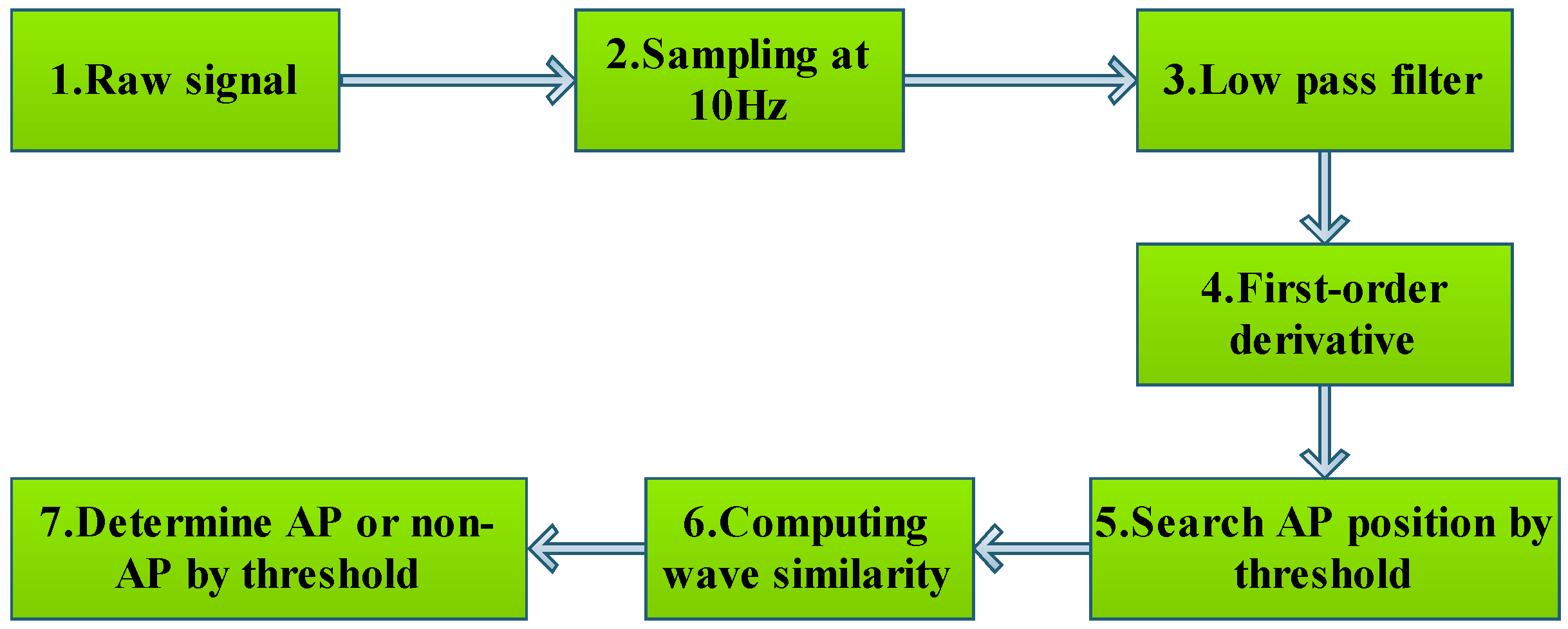
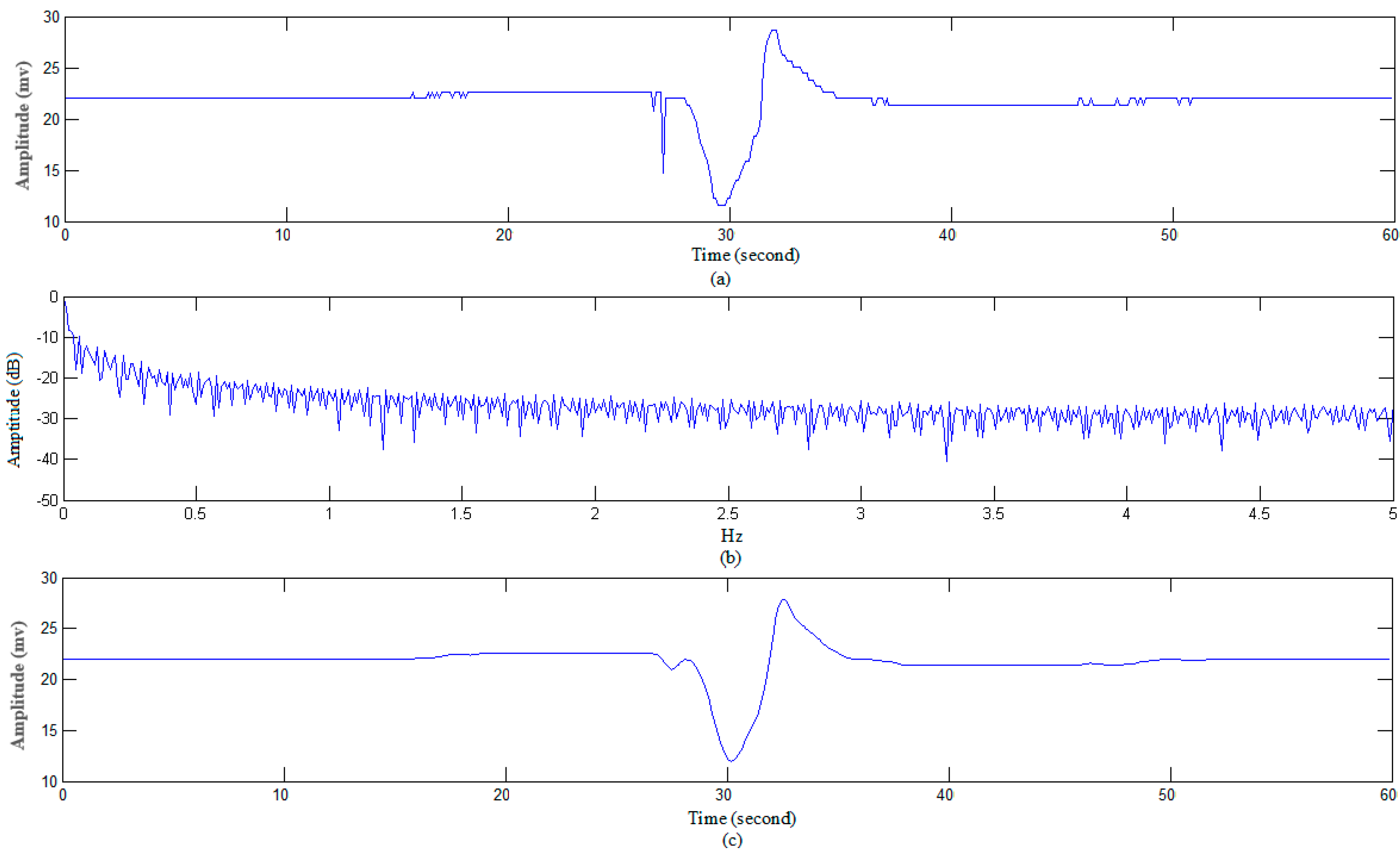
3.1.1. Data Preprocessing

Typically, the frequency of AP in cucumber is less than 1Hz, and then it allows us to reduce data points without distortion by extract at 10 Hz from the raw signal at 800 Hz or 200 Hz sampling frequency. In practice, both filter parameters and filtering criteria are very important, a new literatures provides details of filtering criteria for plant electrical signals [77]. Next, a low pass digital filter was used to remove 50 Hz interference and artifact in original recordings. The filter is written as Equation (1) [78]:

$$y(nT)=2y(nT-T)-y(nT-2T)+x(nT)-2x(nT-6T)+x(nT-12T)$$

(1)

Where the cut-off frequency of the low pass filter is 11 Hz, and the gain is 36.

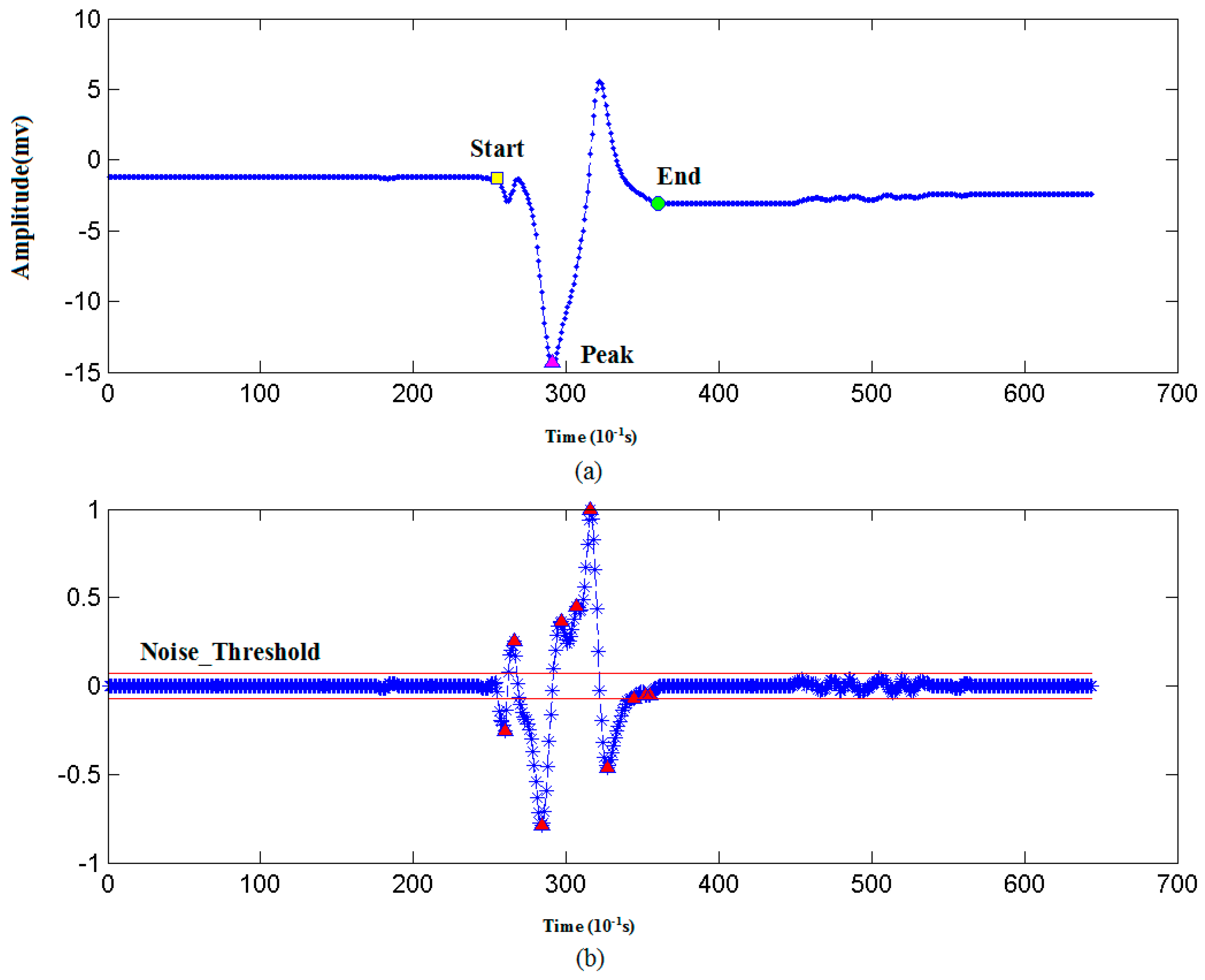
3.1.2. Recognizing Algorithm for Plant Electrical Signals

The APs of plant are aperiodic, and artifacts are similar to APs in shape. For this reason, we have to utilize the time domain processing approach. The AP will become more apparent by performing the first-order derivative for the raw signal. In other words, the first-order derivative algorithm allows us to identify features of AP that are not obvious in the original signal. To recognize AP of plant, our method also considers the both biphasic and monophasic original signal by extracellular recording. Here, monophasic signal is characterized by deflection in one direction, e.g., positive or negative phases [79]. If there are both positive and negative phases to this response, it is referred to as a biphasic signal [80,81].

To determine the starting point, end point, and peak point of signal, the noise peaks threshold is initiated as 0.1 mV/s at first. Then after every first-order derivative, the noise peaks threshold is updated by the following method. We set the new noise peaks threshold as the sum of 0.75× old noise peaks threshold and 0.25× average of new noise peaks.

Using noise peaks threshold, we can obtain all peaks and zero-crossing points which are applied to determine AP peak points, and then search and mark the starting point and end point of AP peak waveform. Based on the information, all waveforms similar to AP can be extracted from raw signal whether they are biphasic or monophasic.

The AP recognition algorithm (Algorithm 1) is as follows:

Algorithm 1: AP extraction.

Input: Raw signal is represented by ST Output: Waveforms similar to AP

BEGIN

1. DS = Take derivative of ST by a five order central difference algorithm // Derivative.

2. Noise_Threshold = 0.1 // Initialize noise threshold.

3. PV = findpeaks(DS) // A search algorithm to find the peaks and valleys in DS.

4. For i=1:N // N is the number of peaks or valleys in PV.

5. IF amplitude of PV(i) < Noise_Threshold THEN N_Peaks = PV(i);   // If peak amplitude is below Noise_Threshold, then add it into N_Peaks.

6. Else S_Peaks = PV(i);   // If peak amplitude is above Noise_Threshold, then add it into S_Peaks.

7. ENDIF

8. END

9. Noise_Threshold = 0.75×Noise_Threshold + 0.25×mean(N_Peaks)   // Update noise threshold

10. For i=1:NS //NS is the number of peaks in S_Peaks

11. S_Peaks_left_Position(i) = Search the left part of S_Peaks(i)   //Search for start point on the left of S_Peaks(i)

12. S_Peaks_right_Position(i) = Search the right part of S_Peaks(i)   // Search for end point on the right of S_Peaks(i)

13. END

14. For i=1:NS-1 //NS is the number of peaks in S_Peaks

15. IF S_Peaks_left_Position(i+1) < S_Peaks_right_Position(i)   // For overlap AP signals, separate them by resetting the end position of last AP and start position of next AP. .

16. THEN   L = S_Peaks_right_Position(i) - S_Peaks_left_Position(i+1);   L1 = L –$\lfloor L/2\rfloor$; L2 = $\lfloor L/2\rfloor$;   S_Peaks_right_Position(i) = S_Peaks_right_Position(i) − L1;   S_Peaks_left_Position(i+1) = S_Peaks_left_Position(i+1) + L2 ;

17. ENDIF

18. END

19. For i=1:NS-1 //NS is the number of peaks in S_Peaks

20. IF Amplitude(S_Peaks(i)) < 5 mv&&Duration(S_Peaks(i))<1s // remove the s_peak point if they meet these conditions

21. THEN Remove S_Peaks(i)

22. ENDIF

23. END

24. For i=1:NS’-1 // NS’ is the number of peaks in S_Peaks

25. IF S_Peaks_left_Position(i+1) == S_Peaks_right_Position(i)||     S_Peaks_left_Position(i+1) == S_Peaks_right_Position(i) + 1   // For adjacent monophasic AP signals, merge them into one APs.

26. THEN // Merge the two APs into one AP    S_Peaks_right_Position(i) = S_Peaks_right_Position(i+1);    Delete S_Peaks(i+1), S_Peaks_left_Position(i+1) and S_Peaks_right_Position(i+1).

27. ENDIF

28. END

29. END

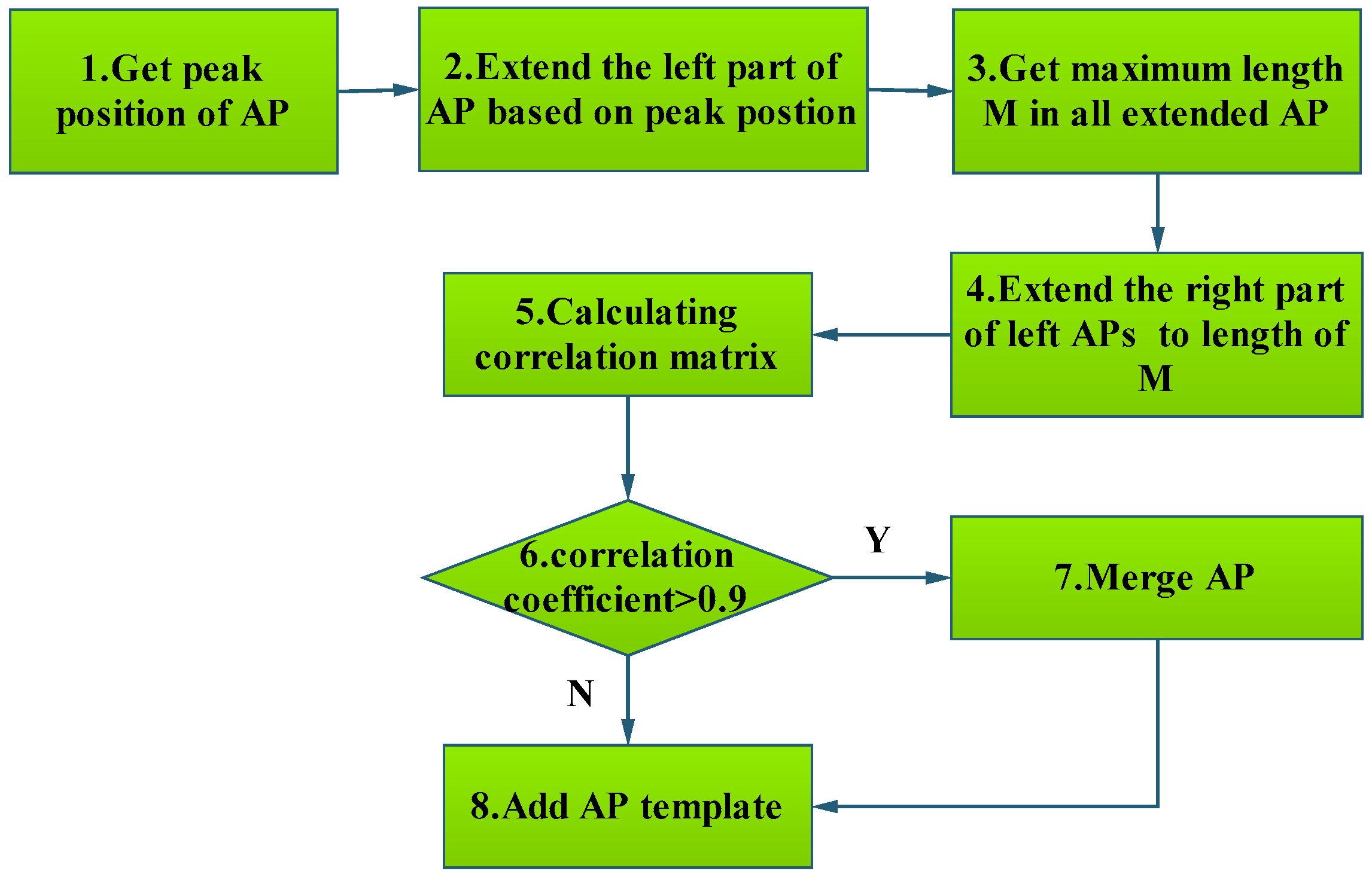
3.1.3. Template Matching Algorithm to Classify AP

Common similarity measure methods for time series include Euclidean distance, dynamic time warping (DTW) [82], as shown in

Table 1. Common similarity measure methods.

Expression	Definition	Advantages	Disadvantages
Euclidean distance $D(X,Y)=\sqrt{{\displaystyle \sum _{i=1}^N{(x_i-y_i)}^2}}$	Calculating the distance of two time series in N-dimensional space	Simple, and supports high-dimensional data	Sensitive to data shift and noise. The length of two time series must be same
DTW $\begin{array}{l}D(x_i,y_i)=DISTANCE(x_i,y_j)+\\ \min [D(x_{i-1},y_j),D(x_i,y_{j-1}),D(x_{i-1},y_{j-1})]\end{array}$	DTW is an algorithm for measuring the similarity between two temporal sequences with different length	Estimate the similarity of two time series with unequal length	O(N2) for computing complexity

. Considering that the extracellular plant AP recordings are relative measurement which depend on the positions of recording electrodes and the reference electrode, so we employed the cross correlation (CC) function. It is a measure of similarity of two time series as a function of the lag of one relative to the other. The length of two time series must be the same. CC is insensitive to amplitude and time shift. It can be expressed as

$$r(d)=\frac{{\displaystyle \sum _i(x_i-\overline{X})(y_{(i-d)}-\overline{Y})}}{\sqrt{{\displaystyle \sum _i{(x_i-\overline{X})}^2}}\sqrt{{\displaystyle \sum _i{(y_{(i-d)}-\overline{Y})}^2}}}$$

(2).

Its value is between −1 and 1. When the delay time in CC is zero (d = 0), it can be used to get Pearson correlation coefficient (PCC) [83]. Here, we selected Pearson correlation coefficient for two reasons. First, it is simple and fast in calculating. Second, it is not affected by the data amplitude and noise. Other similarity methods based on distance measure will be sensitive to noise data, and cannot distinguish AP and non-AP waveform when their amplitudes are close.

We begin with an initial set of N random templates (APs) and the amplitude is transformed to be positive by subtracting the minimum value for every AP, then normalize the APs by Equation (2), and align all peaks based on the peaks’ position by extending all AP waveforms, as shown in Figure 2. Next, we calculate the PCC in Equation (2) to classify the type of APs. If PCC between two APs is bigger than 0.9 (p < 0.01), they are similar, then merge them into one AP by calculating the average value of two APs.

$$X=\frac{X-\min (X)}{max(X)}$$

(3)

$$r=\frac{{\displaystyle \sum _{i=1}^n}(X_i-\overline{X})(Y_i-\overline{Y})}{\sqrt{{\displaystyle \sum _{i=1}^n}{(X_i-\overline{X})}^2}\sqrt{{\displaystyle \sum _{i=1}^n}{(Y_i-\overline{Y})}^2}}$$

(4)

where, $X=\left[X_1,X_2,\dots X_n\right]$, $Y=\left[Y_1,Y_2,\dots Y_n\right]$, $\overline{X}=\frac{1}{n}{\displaystyle \sum _{i=1}^n{X}_i}$, $\overline{Y}=\frac{1}{n}{\displaystyle \sum _{i=1}^n{Y}_i}$.

As mentioned above, it allows us to reduce the numbers of templates by merging templates if PCC is more than 0.9 between the two templates. The new template is generated by calculating the average of two similar templates. There are variations in duration and amplitude between the AP templates, e.g., eight AP templates as shown in Figure 3.

AP classification algorithm (Algorithm 2) is described as follows:

Algorithm 2: Template matching algorithm to classify AP.

Input: Raw signal represented by ST, AP template represented by AT in database

Output: AP, non-AP

1. Normalize ST and AT // Normalize ST and AT by Equation (2)

2. Align ST with AT // STs are properly aligned with templates

Append-Threshold = 0.91; //

Update-threshold = 0.95; //

3. corr = Pearson correlation coefficient between ST and AT // Computing PCC

4. IF corr < Append-Threshold

ST is not an AP signal, reject it.

Return FALSE;

ENDIF

5. IF corr> = Append-Threshold && corr < Update-threshold

Add ST into APTemp // Add ST into AP Template library

Return TURE;

ENDIF

6.IF corr >Update-threshold

Merge ST with APTemp;

Return TURE;

ENDIF

3.1.4. Features Extraction from AP

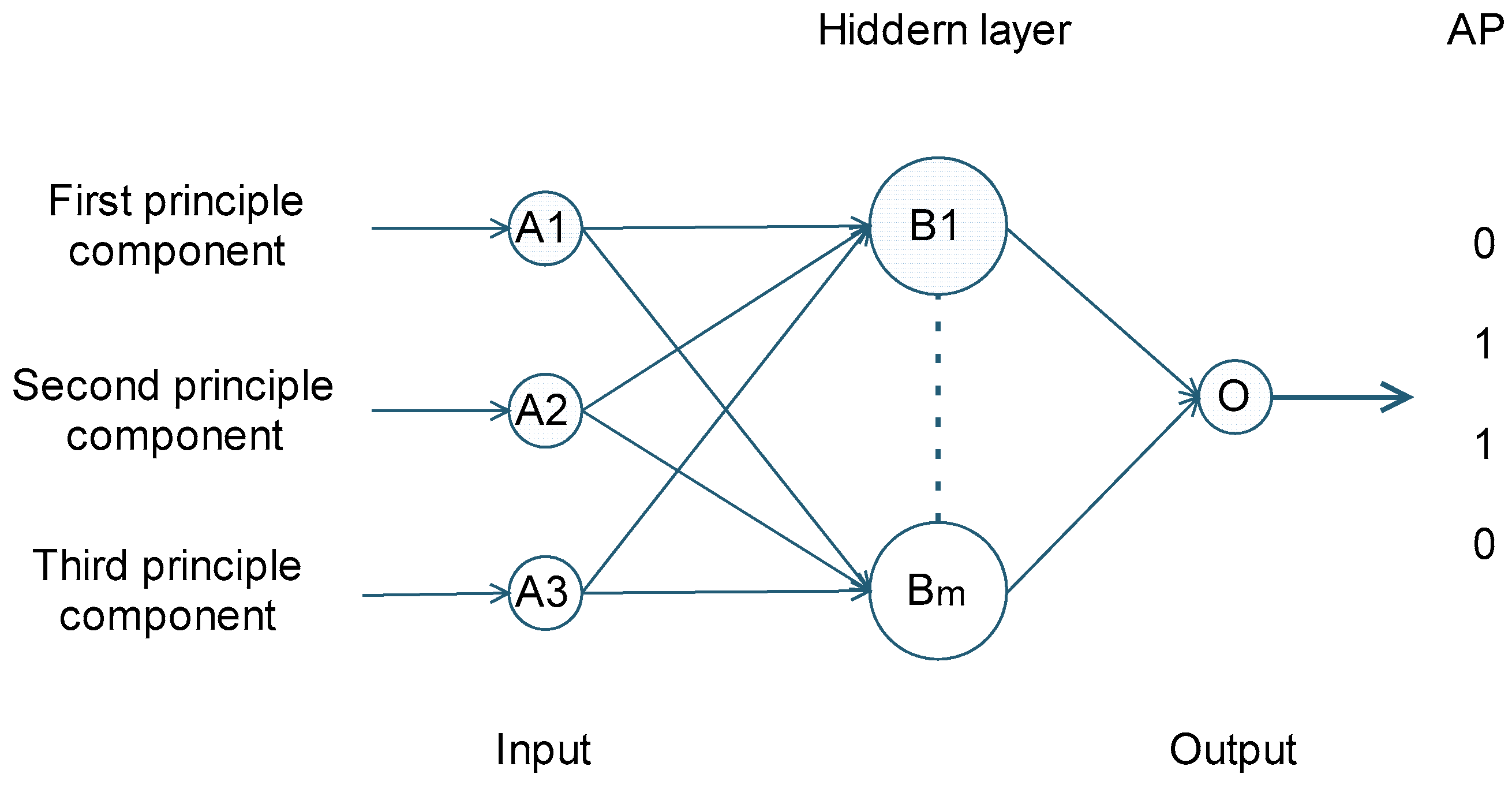
As shown in

Table 2. Features of AP.

Classification	Feature Parameters
Time-domain features (seven items)	Amplitude, Duration, Rising duration, Decline duration, Rising slope, Decline slope, Area
Statistics characteristics (five items)	Skewness, Kurtosis, Hjorth: Hjorth activity, Hjorth mobility, Hjorth complexity
Frequency-domain features (two items)	Average power, Energy
Nonlinear features (five items)	Permutation entropy, Sample entropy, Correlation dimension (CD), LLE, Hurst exponent

, there are 19 parameters of AP waveform which belong to time-domain features, statistical features, frequency-domain features, and nonlinear features.

In this paper, the time-domain and frequency-domain features are defined and calculated in the following description:

AP is considered as time series $X=\left[X_1,X_2,\dots ,X_n\right]$. i is the subscript(index) number of the sampling point, n represents sampling number, the index of peak(valley) is p, $X_p$ is the value of AP at p. The absolute value of amplitude change is defined as Amplitude = |$X_p$ − $X_1$|, $X_1$ is amplitude at the start point. AP duration can be represented by the AP length n. Rising duration is the length from the start position to the peak position of AP represented by p. Decline duration is the length from the peak position to the end position of AP represented by n − p + 1. Rising slope is the ratio of amplitude to rising duration. Assume DP as the absolute difference between the value of peak and the value of the end of AP, then the decline slope is the ratio of DP to decline duration. AP area can be calculated by $Area={\displaystyle \sum _{i=1}^n\left|x_i\right|}$.

3.2. BP-ANNs

BP-ANNs is one of the most popular neural network learning algorithms based on the error backpropagation computing for adjusting net connection weights [84]. The backpropagation algorithm is based on Delta learning rule in which the weight adjustment is performed through mean square error of the output response to the sample input. The set of these sample patterns is repeatedly presented to the network until the error value is minimized. Many researchers use it to cope with the nonlinear problem and a trained backpropagation network is able to detect and classify an input template. It has been used successfully for many applications, e.g., image pattern recognition, medical diagnosis, stock market prediction, and automatic controls.

As is well known, three-layers BP ANNs (Figure 4) is able to approximate any continuous functions [85]. In consequence, this means that one hidden layer-based BP-ANNs can create a new mapping from N-dimensional to M-dimensional. Convergence rate of BP-ANNs increases with the number of hidden nodes. It is worth noting that the increase of number of hidden layers will not necessarily yield to an increase of performance [86]. In this work, based PCA methods [69], the first three principle components of features from AP were used to train the BP-ANNs, namely the number of neurons in the input layer was chosen to be three. One neuron node in output layer was used to classify AP signal.

Therefore, in this paper, considering the convergence rate and fitting accuracy, we compared classification performance using one hidden layer with a different number of hidden nodes respectively. Meanwhile, the Log-sigmoid transfer function is used as the activation functions for both the hidden and output layers, i.e., $f(x)=\frac{1}{1+e^{-x}}$, 0 < f(x) < 1.

3.3. SVM

SVM is a supervised learning algorithm for classification and regression analysis. It is a non-probabilistic binary classifier. It supports both minimizing the empirical classification error and maximizing the geometric margin [87]. It is applied into in various applications such as ECG and EEG signal classification, image classification, text document categorization, etc.

SVM model maps the sample data into another feature spaces so that they can be separated by a hyperplane. A good separation is achieved by the hyperplane that has the largest distance to the nearest training-data point of any class. Kernel functions can be used to measure the relative nearness between the data points to be discriminated to produce maximum-margin hyperplane [87,88,89].

SVM includes linear and nonlinear classifiers which are supported by kernel functions. The common kernel functions are as following [88].

Linear kernel function: $K(x,x_i)=x\cdot x_i$;

Polynomial kernel function: $K(x,x_i)={\left[\left(x\cdot x_j\right)+1\right]}^b$;

Gaussian radial basis function: $K(x,x_i)=\exp (-\frac{|x-x_j{|}^2}{2{\sigma }^2})$;

Sigmoid kernel: $K(x,x_i)=\tanh (\gamma \times (x-x_j)+c)$.

Classification performance is determined by the selection of kernel function and a kernel function’s parameters. In this paper, we compared four kernel functions’ performance to get a proper classifier. Moreover, we tested the results of different kernels with a range of parameters.

3.4. Deep Learning Algorithm

Deep learning approaches attempt to model high-level abstractions in data by using a deep graph with multiple processing layers [90]. It can be used for applications pattern analysis (unsupervised) and classification (supervised) with hierarchical feature extraction.

Common deep learning models [91] include convolutional deep neural networks (DNN), deep belief networks (DBN), Auto encoder (AE), convolutional neural network (CNN), etc. They are have been applied to computer vision, automatic speech recognition, natural language processing, and bioinformatics with a rather good results. DBN proposed by Hilton in 2006 is a directed acyclic graph with multiple layers which is composed of binary or real-valued latent variables.

DBN is a Bayes probabilistic, generative model made up of multiple layers of hidden units. The advantages of DBN are that it is able to learn non-labeled data, train effectively, and overcome the over-fitting.

The basic component in DBN is restricted Boltzmann machines (RBM) which is an undirected, generative energy-based model with a layer of visible units as input layer and a hidden layer. Contrastive divergence (CD) proposed by Hinton is used to train RBMs. In training a single RBM, weight updates are performed with gradient ascent.

DBN can be used for time series predictions—e.g., stock market prediction, speech recognition— and to extract features of electrophysiological data [91]. For this reason, this method is a candidate to deal with APs.

We employed the deep learning tool DeepLearnToolbox (https://github.com/rasmusbergpalm/DeepLearnToolbox) to train the dataset. For setting the parameters of a DBN, mini-batch is set to be equal to the number of categories so that it is easy for parallelism, and each batch consists of a number of samples in a class. In the present work, we classify the plant electrical signal induced by non-damage electrical stimulation into two types: AP and non-AP, mini-batch = 1.There are three hidden layers of our DBN, the number of nodes in the input layer is equal to sampling points of the electrical signal [92].

4. Results

4.1. Classification Results of Our Proposed Method

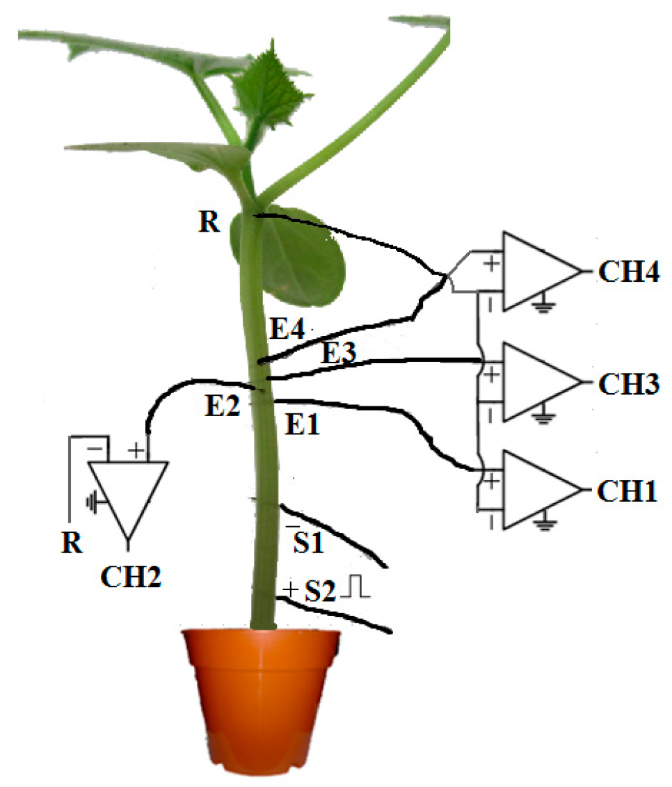
4.1.1. Experimental Data

The details of electrophysiological experiments were performed as described in those previous papers [30,33,36]. Briefly, cucumbers were grown in greenhouse for two to four weeks with 16 h light, 50%–70% humidity, 29 °C in the day and 22 °C at night. For extracellular potential recordings, Ag/AgCl electrodes were 0.2 mm in diameter. When recording, the Ag/AgCl electrodes were inserted into the stem, and the reference electrode was attached to the plant. The extracellular measurements were performed more than 4 h after electrodes inserting. The arrangement of the electrodes is shown in Figure 5.

Two two-channel amplifiers (SWF-1B, ChengDu Instrument factory, Chengdu, China) with signal acquisition system (RM6240, ChengDu Instrument factory, Chengdu, China) were simultaneously used to record the extracellular potential at four positions with 0.2–0.3 cm apart. The plant was placed on an anti-vibration table in a faraday cage (Inbio Life Science Instrument Co., Ltd., Wuhan, China).

The electrical stimulus was applied by current injection. Two platinum wire electrodes, 0.1 mm diameter, 1.5 cm apart were inserted in the stem, 2 cm apart from the recording electrode. 2–15 V, 0.05–2 s squared DC pulse were applied through the platinum wire. In fact, the strength-duration curve allows us to determine the rheobase and the chronaxy value [79,80]. For the same plant, the next stimulus was applied for at least 3 h if there are multiple current injections.

After current injections, 68 data files were recorded with 32 plant samples. The Aps’ amplitude was from 10 mV to 80 mV with duration time from 2 s to 30 s. As the frequency of AP is lower than 1 Hz (Figure 6b), a low-pass filter was used to reduce the current injection artifacts (Figure 6c).

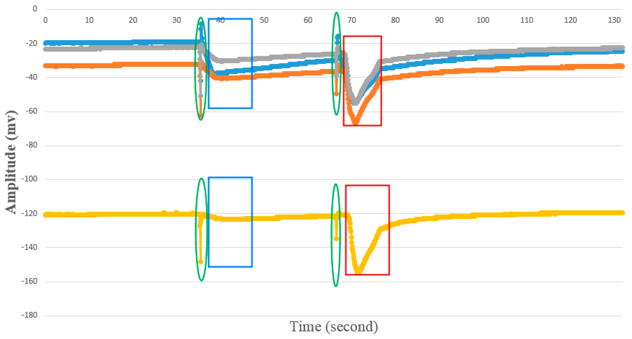
4.1.2. AP Waveform Recognition Results

Figure 7a shows the filtered signal after attenuating noise. The detected AP waveform position is marked in Figure 7a which contains the start position, peak position, and end position. The whole waveform contains stimulus artifact and AP signals in Figure 7a. It is reasonable for the stimulus artifact often occurs at the start of AP signals. Figure 7b is the derivative signal. We used the adaptive noise threshold to eliminate noise peaks in signal. Then we can search the left peaks and troughs which marked with triangles in Figure 7a. The zero-cross points between the peaks and troughs are corresponding to peaks or troughs in raw signals. After careful processing, we got all possible peaks of waveforms similar to AP from these zero-cross points. Then we search the start and end positions of the peaks.

Although we extracted 329 waveforms like AP from raw data, there were still existing 96 artifacts signals or non-standard APs among them. Therefore, we need a more accurate classification method to recognize standard AP.

4.1.3. Template Matching Results

We tested the 329 AP and non-AP waveforms described in Section 4.1 and Section 4.2. To get a better threshold when adding new template or updating the template library, we compared different thresholds and select the threshold which showed the best performance. As shown in

Table 3. Different thresholds for template matching algorithm.

Append-Threshold	Update-Threshold	Accuracy	The Number of New Templates
0.89	0.95	95.4%	38
0.9	0.95	95.4%	27
0.91	0.95	96.0%	24
0.92	0.95	95.7%	21
0.93	0.95	92.1%	19
0.94	0.95	87.5%	13
0.95	0.96	85.4%	13

, we set different thresholds for every training and got different results. If the threshold for adding new templates is too small, the probability of adding non-AP as template will get bigger and the number of template library will increase fast. If it is too big, there will be few templates added into the template library, producing a low accuracy. Here, we set Append-Threshold = 0.91, and Update-threshold = 0.95 to get the best performance which classification rate is 96.0%.

4.1.4. Features of AP waveforms

Based on the APs characteristics and priori knowledge [1,2,3,4,5,6,8], 329 raw signals were divided into two classes: AP and non-AP. Moreover, non-AP include artifacts, subthreshold response, noise, transient interference, VPs, etc. As shown in Figure 8, there is a typical case of the observed raw signals induced by electrical stimulation, which consist of artifacts, subthreshold responses, and APs.

We extracted 19 features from 329 waveforms which include 96 non-AP waveforms and 233 standard AP waveforms. To test significant difference between every feature of AP and non-AP, we employed T-test (p < 0.05) (

Table 4. T-test for non-AP and AP features.

Features	Non-AP (Mean ± S.E.M.)	AP (Mean ± S.E.M.)
Amplitude * (mV)	14.33 ± 9.90	20.57 ± 12.55
Durations * (s)	8.01 ± 4.35	9.75 ± 5.05
Rising duration * (s)	2.36 ± 1.31	3.00 ± 1.62
Decline duration * (s)	5.75 ± 3.61	6.85 ± 4.22
Rising slope * (mv/s)	6.78 ± 6.19	8.42 ± 7.47
Decline slope (mv/s)	2.64 ± 2.13	2.90 ± 2.61
Area	4749.01 ± 7728.3	6078.16 ± 11,038.49
Skewness	−0.57 ± 0.71	−0.50 ± 0.65
Kurtosis	2.80 ± 1.33	2.70 ± 0.82
Hjorth activity *	27.27 ± 34.44	48.82 ± 54.37
Hjorth mobility *	0.16 ± 0.10	0.14 ± 0.07
Hjorth complexity *	1.89 ± 0.71	2.17 ± 0.91
Energy *	740,601.4 ± 1,415,709	1,207,443 ± 2,076,630
Average power *	8065.49 ± 15,968.75	11,440.17 ± 18,881.54
Permutation entropy	0.83 ± 0.25	0.82 ± 0.19
Sample entropy	0.05 ± 0.05	0.05 ± 0.05
Correlation dimension	0.75 ± 0.24	0.74 ± 0.22
LLE *	−0.07 ± 0.07	−0.05 ± 0.04
Hurst	0.99 ± 0.07	0.99 ± 0.04

* Statistically significant difference (p < 0.05) between Non-AP and AP. S.E.M. is standard error of the mean.

).

T-test results show that there is a statistical difference in the average value of features between AP and non-AP including duration, left duration, right duration, left slope, amplitude, energy, power, LLE, Hjorth activity, Hjorth mobility, and Hjorth complexity. The rest features do not show a significant difference. Hence, we just selected the 11 features which show significant difference for classification.

Only LLE shows real difference among non-linear features. LLE of AP and non-AP are all below zero which represents that the AP time series is not a chaotic process in this paper. The Hurst exponent of AP showed that AP signals are more stable and predictable.

4.2. Classification Results of BP-ANNs

A testing dataset including 329 samples of AP and non-AP is described in Section 4.1. We employed the neural network tool provided by Matlab 2014a. BP neural network in the test is a typical three-layer network. The 11 features were reduced to 3 by PCA method. We select the first three principal components which percentage sum is approximate 91.7% (

Table 5. Features reduction by PCA.

	First Principle Component	Second Principle Component	Third Principle Component	Fourth Principle Component	Fifth Principle Component
Eigenvalue	0.2700	0.0770	0.0285	0.0128	0.0078
Percentage	65.89%	18.80%	6.96%	3.13%	1.91%
Accumulated percentage	65.89%	84.68%	91.65%	94.78%	96.69%

).

Before training the data, all data will be normalized. The normalized method is X = 2 × (X − min(X))/(max(X) − min(X)) − 1. Two-thirds of the dataset are randomly selected to train the BP neural network, and one-third of data are for testing. The 10-fold cross validation was used to train the data. The results showed that the maximum accuracy 84.8% was achieved when the number of units in the hidden layer is 8. The classification accuracy with different hidden unit number is shown in

Table 6. Performance of three-layer BP neural network with different hidden units.

Units Number	Accuracy	Run Time
20	79.7%	2704 s
16	84.8%	5340 s
12	81.5%	34,727 s
8	84.1%	65,664 s
4	83.5%	20,687 s

.

4.3. Classification Results of SVM

As described in Section 4.4, we used PCA method to reduce the features dimension. Then we used the SVM tool provided by Matlab 2014a. Two-thirds of the dataset are selected randomly to train the SVM, and one-third of the data are for testing. The 10-fold cross validation was used to train the data.

Firstly, we used the linear kernel in SVM for classification.

Table 7. Results of different components for SVM classification.

	First Principle Component	Second Principle Component	Third Principle Component	Fourth Principle Component	Fifth Principle Component
Accuracy	55.6%	66.7%	75.8%	76.7%	77.3%

shows the classification results with different components.

We just select the first three principal components for simplification, and the accuracy is 75.8%. Figure 9 shows the first two principal components scatter plot and 3-D scatter plot of first three principal components of AP and non-AP. The red letter “+” represents the non-AP features, and blue circle “o” represents the AP features. From the figures, we see that two kinds of data are mixed and not easily divided by the linear classifier.

In addition, we also tested other nonlinear kernel functions. As shown in

Table 8. Different kernel functions for classification.

Kernel Function	Range of Parameters	Interval	Selected Parameters	Highest Accuracy
Quadratic kernel ${\left[\left(x_i\cdot x_j\right)+1\right]}^b$	b = 2	0	b = 2	62.96%
Polynomial kernel ${\left[\left(x_i\cdot x_j\right)+1\right]}^b$	b = 3	0	b = 3	74.07%
Gaussian Radial Basis Function $\exp (-\frac{|x_i-x_j{|}^2}{2{\sigma }^2})$	$\sigma =[0.1,3]$	0.1	$\sigma =1.9$	77.59%
Sigmoid kernel $\tanh (\gamma \times (x_i-x_j)+c)$	$\gamma =[0.1,5]$ $c=[-5,-0.1]$	0.1	$\gamma =0.1$ c = −0.3	78.17%

, we found that the sigmoid kernel function has the best performance in the classification with 78.2% accuracy.

To get best parameters, we set the range of every parameter at increasing intervals and then trained the dataset with them.

4.4. Classification Results of Deep Learning Method

To make the length of all waveforms same, the 329 AP and non-AP waveforms were aligned at the peak points of these waveforms, then all waveforms are extended on the left and right of the peak.

As similar to Section 4.4, two-thirds of the dataset were randomly selected to train the DBN, and one-third of data were for testing. The 10-fold cross validation was used to train the data.

To get a better classification performance, we tried different network structure settings as shown in

Table 9. Different parameters for DBN.

	Number of Second Hidden Units	Number of Third Hidden Units	Number of Fourth Hidden Units	Selected Parameters	Highest Accuracy
Range	[40, 200]	[8, 24]	[4, 8]	Multiple selections	77.4% (3 hidden layers)
Interval	40	4	4	Multiple selections	77.4% (4 hidden layers)

. For three hidden layers, the best performance is 77.4% which is corresponding to multiple optional parameter settings. For four hidden layers, the best performance is 77.4% too. By comparing different numbers of hidden layers and units, we got the highest accuracy of 77.4%.

5. Discussion

In the same plant, there is no variation in the parameters of AP—e.g., amplitude, duration—once a critical membrane potential threshold is exceeded. However, there are variations in different plants. Although the parameters of the APs evoked by electrical stimulation were highly variable (range 10–80 mV, duration time from 2 s to 30 s), once a critical membrane potential threshold is exceeded, it was related neither to the intensity nor to the duration of the stimulation pulse, namely the phenomenon is a typical all-or-nothing response. Similar results were reported by others [79]. The results also suggested that our template matching algorithm is potential useful tool to classify these various waveforms of APs. Furthermore, it is worth studying the mechanism of variations in APs among these individuals in the future.

In

Table 10. Comparison of four classifiers.

Classifier	Accuracy	Average Running Time	Sensitivity	Specificity	Positive Predictive Value (PPV)	Negative Predictive Value (NPV)
Template matching	96.0%	3.20 s	96.6%	94.8%	97.8%	91.9%
BP neural network	84.8%	5340 s	74.9%	52%	89.7%	27.1%
SVM	78.2%	2.1 s	89.5%	95.8%	98.7%	7.2%
DBN	77.4%	112.06 s	100%	0	70.8%	0

, we compared four classifiers performance. Here, we assume TP (true positive) as the APs detected, FP (false positive) indicates that classifying the non-AP as AP, TN (true negative) indicates that non-APs were classified as non-AP, FN (false negative) indicates that classifying the APs as non-AP.

Then, the sensitivity or true positive rate can be expressed as $sensitivity=\frac{TP}{TP+FN}$. The specificity or true negative rate can be expressed as $specificity=\frac{TN}{TN+FP}$. The positive predictive value can be expressed as $PPV=\frac{TP}{TP+FP}$. The negative predictive value is $NPV=\frac{TN}{TN+FN}$.

It is clear that template matching is the best classifier among them. Although the accuracy of BP neural networks reached 85.18%, its training time is very long and it cannot distinguish the non-AP. Moreover, users have to select proper parameters by comparing classification performance in many tests with difference parameters. SVM is an efficient classifier for its short running time. The results show that SVM cannot recognize non-AP correctly. Users have to select or construct a proper kernel function and try to optimize parameters to get better results. Deep learning is a potential good choice though its accuracy is lowest. All AP were detected, but all non-AP were treated as AP. The dataset may be still small for deep learning in this paper. In addition, DBN can be used to extract key feature vectors from the dataset, then these features can be trained by other classifiers such as SVM. By combining other classifiers, DBN may have better results.

In this paper, template matching method is the most reasonable method for higher PPV and NPV. The time costs depend on calculating coefficients which time complexity is O(N). It has generalization capacity with the increase of data, but when the template library gets larger, it will need more time to matching different templates. To get a good accuracy and keep the template number from increasing so fast, it is very important to adjust the two thresholds in template matching when adding and updating the templates.

Furthermore, reducing the matching time is a more sophisticated problem, and false templates may be added into the template library, how to keep a standard template library is another important problem.

In other application scenarios, there were even composite signals involving both APs and VPs induced by strong damage such as burning. In fact, as a versatile new way, our proposed method is able to extract peaks from process of a VP induced by heat-wounding, for which the data was published in 1998 by Stankovic and his coauthors [93]. Next, the extracted peaks could be classified by template matching algorithm. Results were shown in the supplementary Figure S1. Furthermore, systemic study for identifying and classification of VPs is our future work.

6. Conclusions

In this paper, we combined AP recognition algorithm and template matching algorithm to identify and classify extracellular APs when there are noise, stimulus artifacts, and variability of signals. These results suggest that our template matching algorithm has the highest classification accuracy compared with the BP neural network method, deep learning method, and SVM. In the future, we will improve the template matching algorithm by designing fast waveform index for template library to decrease the matching time and increase accuracy. All these methods can be potentially used to rapidly classify and search plant electrical signal in a large scale standard plant electrical signals database for data sharing, interpretation, and applications research.

References

1. Trebacz, K.; Dziubinska, H.; Krol, E. Electrical signals in long-distance communication in plants. In Communication in Plants; Baluska, F., Mancuso, S., Volkmann, D., Eds.; Springer: Berlin/Heidelberg, Germany; New York, NY, USA, 2006; pp. 277–290. [Google Scholar]
2. Yan, X.; Wang, Z.; Huang, L.; Wang, C.; Hou, R.; Xu, Z.; Qiao, X. Research progress on electrical signals in higher plants. Prog. Nat. Sci. 2009, 19, 531–541. [Google Scholar] [CrossRef]
3. Król, E.; Dziubinska, H.; Trebacz, K. What do plants need action potentials? In Action Potential: Biophysical and Cellular Context, Initiation, Phases and Propagation; Dubois, M.L., Ed.; Nova Science Publisher: New York, NY, USA, 2010; pp. 1–26. [Google Scholar]
4. Fromm, J.; Lautner, S. Generation, Transmission, and Physiological Effects of Electrical Signals in Plants. In Plant Electrophysiology-Signaling and Responses; Volkov, A.G., Ed.; Springer: Berlin/Heidelberg, Germany; New York, NY, USA, 2012; pp. 207–232. [Google Scholar]
5. Gallé, A.; Lautner, S.; Flexas, J.; Fromm, J. Environmental stimuli and physiological responses: The current view on electrical signalling. Environ. Exp. Bot. 2015, 114, 15–21. [Google Scholar] [CrossRef]
6. Vodeneev, V.A.; Katicheva, L.A.; Sukhov, V.S. Electrical signals in higher plants: Mechanisms of generation and propagation. Biophysical 2016, 61, 505–512. [Google Scholar] [CrossRef]
7. Zimmermann, M.R.; Maischak, H.; Mithoefer, A.; Boland, W.; Felle, H.H. System potentials, a novel electrical long-distance apoplastic signal in plants, induced by wounding. Plant Physiol. 2009, 149, 1593–1600. [Google Scholar] [CrossRef] [PubMed]
8. Sukhov, V.; Nerush, V.; Orlova, L.; Vodeneev, V. Simulation of action potential propagation in plants. J. Theor. Biol. 2011, 291, 47–55. [Google Scholar] [CrossRef] [PubMed]
9. Sukhov, V.; Akinchits, E.; Katicheva, L.; Vodeneev, V. Simulation of Variation Potential in Higher Plant Cells. J. Membr. Biol. 2013, 246, 287–296. [Google Scholar] [CrossRef] [PubMed]
10. Davies, E. New functions for electrical signals in plants. New Phytol. 2004, 161, 607–610. [Google Scholar] [CrossRef]
11. Fromm, J.; Lautner, S. Electrical signals and their physiological significance in plants. Plant. Cell Environ. 2007, 30, 249–257. [Google Scholar] [CrossRef] [PubMed]
12. Stahlberg, R.; Stephens, N.R.; Cleland, R.E.; Volkenburgh, E.V. Shade-Induced Action Potentials in Helianthus annuus L. Originate Primarily from the Epicotyl. Plant Signal Behav. 2006, 1, 15–22. [Google Scholar] [CrossRef] [PubMed]
13. Favre, P.; Greppin, H.; Agosti, R.D. Accession-dependent action potentials in Arabidopsis. J. Plant Physiol. 2011, 168, 653–660. [Google Scholar] [CrossRef] [PubMed]
14. Pavlovic, A.; Slovakova, L.; Pandolfi, C.; Mancuso, S. On the mechanism underlying photosynthetic limitation upon trigger hair irritation in the carnivorous plant Venus flytrap (Dionaea muscipula Ellis). J. Exp. Bot. 2011, 62, 1991–2000. [Google Scholar] [CrossRef] [PubMed]
15. Sukhov, V.; Surova, L.; Sherstneva, O.; Katicheva, L.; Vodeneev, V. Variation potential influence on photosynthetic cyclic electron flow in pea. Front. Plant Sci. 2015, 5. [Google Scholar] [CrossRef] [PubMed]
16. Krupenina, N.A.; Bulychev, A.A. Action potential in a plant cell lowers the light requirement for non-photochemical energydependent quenching of chlorophyll fluorescence. Biochim. Biophys. Acta 2007, 1767, 781–788. [Google Scholar] [CrossRef] [PubMed]
17. Sukhov, V.; Sherstneva, O.; Surova, L.; Katicheva, L.; Vodeneev, V. Proton cellular influx as a probable mechanism of variation potential influence on photosynthesis in pea. Plant. Cell Environ. 2014, 37, 2532–2541. [Google Scholar] [CrossRef] [PubMed]
18. Sukhov, V.; Surova, L.; Morozova, E.; Sherstneva, O.; Vodeneev, V. Changes in H+-ATP synthase activity, proton electrochemical gradient, and pH in pea chloroplast can be connected with variation potential. Front. Plant Sci. 2016, 7. [Google Scholar] [CrossRef] [PubMed]
19. Lautner, S.; Stummer, M.; Matyssek, R.; Fromm, J.; Grams, T.E.E. Involvement of respiratory processes in the transient knockout of net CO2 uptake in Mimosa pudica upon heat stimulation. Plant. Cell Environ. 2014, 37, 254–260. [Google Scholar] [CrossRef] [PubMed]
20. Surova, L.; Sherstneva, O.; Vodeneev, V.; Katicheva, L.; Semina, M.; Sukhov, V. Variation potential-induced photosynthetic and respiratory changes increase ATP content in pea leaves. J. Plant Physiol. 2016, 202, 57–64. [Google Scholar] [CrossRef] [PubMed]
21. Grams, T.E.E.; Koziolek, C.; Lautner, S.; Matyssek, R.; Fromm, J. Distinct roles of electric and hydraulic signals on the reaction of leaf gas exchange upon re-irrigation in Zea mays L. Plant. Cell Environ. 2007, 30, 79–84. [Google Scholar] [CrossRef] [PubMed]
22. Sukhov, V.; Surova, L.; Sherstneva, O.; Bushueva, A.; Vodeneev, V. Variation potential induces decreased PSI damage and increased PSII damage under high external temperatures in pea. Funct. Plant Biol. 2015, 42, 727–736. [Google Scholar] [CrossRef]
23. Maffei, M.E.; Mithofer, A.; Boland, W. Before gene expression: Early events in Plant-insect interaction. Trends Plant Sci. 2007, 12, 310–316. [Google Scholar] [CrossRef] [PubMed]
24. Hedrich, R.; Salvador-Recatala, V.; Dreyer, I. Electrical Wiring and Long-Distance Plant Communication. Trends Plant Sci. 2016, 21, 376–387. [Google Scholar] [CrossRef] [PubMed]
25. Großkinsky, D.K.; Svensgaard, J.; Christensen, S.; Roitsch, T. Plant phenomics and the need for physiological phenotyping across scales to narrow the genotype-to-phenotype knowledge gap. J. Exp. Bot. 2015, 66, 5429–5440. [Google Scholar]
26. Fiorani, F.; Schurr, U. Future Scenarios for Plant Phenotyping. Annu. Rev. Plant Biol. 2013, 64, 267–291. [Google Scholar] [CrossRef] [PubMed]
27. Mousavi, S.A.; Chauvin, A.; Pascaud, F.; Kellenberger, S.; Farmer, E.E. Glutamate Receptor-Like genes mediate leaf-to-leaf wound signalling. Nature 2013, 500, 422–426. [Google Scholar] [CrossRef] [PubMed]
28. Felle, H.H.; Zimmermann, M.R. Systemic signalling in barley through action potentials. Planta 2007, 226, 203–214. [Google Scholar] [CrossRef] [PubMed]
29. Agosti, R.D. Touch-induced action potentials in Arabidopsis thaliana. Arch. Des. Sci. J. 2014, 67, 125–138. [Google Scholar]
30. Macedo, F.C.O.; Dziubinska, H.; Trebacz, K.; Oliveira, R.F.; Moral, R.A. Action potentials in abscisic acid-deficient tomato mutant generated spontaneously and evoked by electrical stimulation. Acta Physiol. Plant 2015, 37, 1–9. [Google Scholar] [CrossRef]
31. Mancuso, S. Hydraulic and electrical transmission of wound-induced signals in Vitis vinifera. Aust. J. Plant Physiol. 1999, 26, 55–61. [Google Scholar] [CrossRef]
32. Stahlberg, R.; Cosgrove, D.J. A reduced xylem pressure altered the electric and growth responses in cucumber hypocotyls. Plant Cell Environ. 2008, 20, 101–109. [Google Scholar] [CrossRef]
33. Volkov, A.G.; Adesina, T.; Jovanov, E. Closing of Venus flytrap by electrical stimulation of motor cells. Plant Signal. Behav. 2007, 3, 139–145. [Google Scholar] [CrossRef]
34. Van Bel, A.J.E.; Ehlers, K. Electrical Signalling via Plasmodesmata. In Plasmodesmata; Oparka, K.J., Ed.; Blackwell Publishing Ltd.: Oxford, UK, 2005; pp. 263–278. [Google Scholar] [CrossRef]
35. Huang, L.; Wang, Z.Y.; Xu, Z.L.; Liu, Z.C.; Zhao, Y.; Hou, R.F.; Wang, C. Design of Multi-channel Monitoring System for Electrical Signals in Plants. Mod. Sci. Instrum. 2006, 4, 45–47. (In Chinese) [Google Scholar]
36. Zhao, D.J.; Chen, Y.; Wang, Z.Y.; Xue, L.; Mao, T.L.; Liu, Y.M.; Wang, Z.Y.; Huang, L. High-resolution non-contact measurement of the electrical activity of plants in situ using optical recording. Sci. Rep. 2015, 5, 1–14. [Google Scholar] [CrossRef] [PubMed]
37. Parisot, C.; Agosti, R.D. Fast acquisition of action potentials in Arabidopsis thaliana. Arch. Des. Sci. J. 2014, 67, 139–148. [Google Scholar]
38. Masi, E.; Ciszak, M.; Stefano, G.; Renna, L.; Azzarello, E.; Pandolfi, C.; Mugnai, S.; Baluška, F.; Arecchi, F.T.; Mancuso, S. Spatiotemporal dynamics of the electrical network activity in the root apex. Proc. Natl. Acad. Sci. USA 2009, 106, 4048–4053. [Google Scholar] [CrossRef] [PubMed]
39. Kalovrektis, K.; Th, G.; Antonopoulos, J.; Gotsinas, A.; Shammas, N.Y.A. Development of Transducer Unit to Transmit Electrical Action Potential of Plants to A Data Acquisition System. Am. J. Bioinform. Res. 2013, 3, 21–24. [Google Scholar]
40. Gil, P.M.; Gurovich, L.; Schaffer, B.; Alcayaga, J.; Rey, S.; Iturriaga, R. Root to leaf electrical signaling in avocado in response to light and soil water content. J. Plant Physiol. 2008, 165, 1070–1078. [Google Scholar] [CrossRef] [PubMed]
41. Salvador-Recatala, V.; Tjallingii, W.F.; Farmer, E.E. Real-time, in vivo recordings of caterpillar-induced waves in sieve elements using aphid electrodes. New Phytol. 2014, 203, 674–684. [Google Scholar] [CrossRef] [PubMed]
42. Zhang, X.H.; Yu, N.M.; Xi, G.; Meng, X. Changes in the power spectrum of electrical signals in maize leaf induced by osmotic stress. Chin. Sci. Bull. 2012, 57, 413–420. [Google Scholar] [CrossRef]
43. Huang, L.; Wang, Z.Y.; Zhao, L.L.; Zhao, D.J.; Wang, C.; Xu, Z.L.; Hou, R.F.; Qiao, X.J. Electrical signal measurement in plants using blind source separation with independent component analysis. Comput. Electron. Agric. 2010, 71, S54–S59. [Google Scholar] [CrossRef]
44. Zhao, D.J.; Wang, Z.Y.; Li, J.; Wen, X.; Liu, A.; Huang, L.; Wang, X.D.; Hou, R.F.; Wang, C. Recording extracellular signals in plants: A modeling and experimental study. Math. Comput. Model. 2013, 58, 556–563. [Google Scholar] [CrossRef]
45. Aditya, K.; Chen, Y.L.; Kim, E.H.; Udupa, G.; Lee, Y.K. Development of Bio-machine based on the plant response to external stimuli. In Proceedings of the 2011 IEEE International Conference on Robotics and Biomimetics (ROBIO), Shanghai, China, 9–13 May 2011; pp. 1218–1223.
46. Yang, R.; Lenaghan, S.C.; Li, Y.F.; Oi, S.; Zhang, M.J. Mathematical Modeling, Dynamics Analysis and Control of Carnivorous Plants. In Plant Electrophysiology; Alexander, G.V., Ed.; Springer: Berlin/Heidelberg, Germany; New York, NY, USA, 2012; pp. 63–83. [Google Scholar]
47. Chatterjee, S.; Das, S.; Maharatna, K.; Masi, E.; Santopolo, L.; Mancuso, S.; Vitaletti, A. Exploring strategies for classification of external stimuli using statistical features of the plant electrical response. J. R. Soc. Interface 2015, 12. [Google Scholar] [CrossRef] [PubMed]
48. Chatterjee, S.K.; Ghosh, S.; Das, S.; Manzella, V.; Vitaletti, A.; Masi, E.; Santopolo, L.; Mancuso, S.; Maharatna, K. Forward and Inverse Modelling Approaches for Prediction of Light Stimulus from Electrophysiological Response in Plants. Measurement 2014, 53, 101–116. [Google Scholar] [CrossRef]
49. Lanata, A.; Guidi, A.; Baragli, P.; Valenza, G.; Scilingo, E.P. A Novel Algorithm for Movement Artifact Removal in ECG Signals Acquired from Wearable Systems Applied to Horses. PLoS ONE 2015, 10, e0140783. [Google Scholar] [CrossRef] [PubMed]
50. Khatun, S.; Mahajan, R.; Morshed, B.I. Comparative Study of Wavelet-Based Unsupervised Ocular Artifact Removal Techniques for Single-Channel EEG Data. IEEE J. Transl. Eng. Health Med. 2016, 4, 1–8. [Google Scholar] [CrossRef] [PubMed]
51. Manikandan, M.S.; Soman, K.P. A novel method for detecting R-peaks in electrocardiogram (ECG) signal. Biomed. Signal Process. 2012, 7, 118–128. [Google Scholar] [CrossRef]
52. Satija, U.; Ramkumar, B.; Manikandan, M.S. A simple method for detection and classification of ECG noises for wearable ECG monitoring devices. In Proceedings of the Second IEEE International Conference on Signal Processing and Integrated Networks (SPIN), Greater Noida, India, 19–20 February 2015.
53. Liu, S.H. Motion artifact reduction in electrocardiogram using adaptive filter. J. Med. Biol. Eng. 2011, 31, 67–72. [Google Scholar] [CrossRef]
54. Wessel, J.R. Testing Multiple Psychological Processes for Common Neural Mechanisms Using EEG and Independent Component Analysis. Brain Topogr. 2016. [Google Scholar] [CrossRef] [PubMed]
55. Poungponsri, S.; Yu, X.H. An adaptive filtering approach for electrocardiogram (ECG) signal noise reduction using neural networks. Neurocomputing 2013, 117, 206–213. [Google Scholar] [CrossRef]
56. Arbateni, K.; Bennia, A. Sigmoidal radial basis function ANN for QRS complex detection. Neurocomputing 2014, 145, 438–450. [Google Scholar] [CrossRef]
57. Kabir, M.A.; Shahnaz, C. Denoising of ECG signals based on noise reduction algorithms in EMD and wavelet domains. Biomed. Signal Process. 2012, 7, 481–489. [Google Scholar] [CrossRef]
58. Bhateja, V.; Verma, R.; Mehrotra, R.; Urooj, S. A Non-linear Approach to ECG Signal Processing using Morphological Filters. Int. J. Meas. Technol. Instrum. Eng. (IJMTIE) 2013, 3, 46–59. [Google Scholar] [CrossRef]
59. Zhang, F.; Lian, Y. QRS Detection Based on Multiscale Mathematical Morphology for Wearable ECG Devices in Body Area Networks. IEEE Trans. Biomed. Circuits Syst. 2009, 3, 220–228. [Google Scholar] [CrossRef] [PubMed]
60. Arzeno, N.M.; Deng, Z.D.; Poon, C.S. Analysis of first-derivative based QRS detection algorithms. IEEE Trans. Biomed. Eng. 2008, 55, 478–484. [Google Scholar] [CrossRef] [PubMed]
61. Kim, J.; Shin, H. Simple and Robust Realtime QRS Detection Algorithm Based on Spatiotemporal Characteristic of the QRS Complex. PLoS ONE 2016, 11. [Google Scholar] [CrossRef] [PubMed]
62. Riedl, M.; Müller, A.; Wessel, N. Practical considerations of permutation entropy: A tutorial review. Eur. Phys. J. Spec. Top. 2013, 222, 249–262. [Google Scholar] [CrossRef]
63. Richman, J.S.; Lake, D.E.; Moorman, J.R. Sample Entropy. Method Enzymol. 2004, 384, 172–184. [Google Scholar]
64. Silva, C.; Pimentel, I.R.; Andrade, A.; Foreid, J.P.; Ducla-Soares, E. Correlation Dimension Maps of EEG from Epileptic Absences. Brain Topogr. 1999, 11, 201–209. [Google Scholar] [CrossRef] [PubMed]
65. Kocarev, L.; Tasev, Z. Lyapunov exponents, noise-induced synchronization, and Parrondo’s paradox. Phys. Rev. E 2002, 65, 046215. [Google Scholar] [CrossRef] [PubMed]
66. Wolf, A.; Swift, J.B.; Swinney, H.L.; Vastano, J.A. Determining Lyapunov exponents from a time series. Phys. D 1985, 16, 285–317. [Google Scholar] [CrossRef]
67. Stefański, A. Determining Thresholds of Complete Sychronization and Application; World Scientific: Singapore, 2009. [Google Scholar]
68. Martinis, M.; Knezević, A.; Krstacić, G.; Vargović, E. Changes in the Hurst exponent of heartbeat intervals during physical activity. Phys. Rev. E Stat. Nonlinear Soft Matter Phys. 2002, 70, 127–150. [Google Scholar] [CrossRef] [PubMed]
69. Martis, R.J.; Acharya, U.R.; Min, L.C. ECG beat classification using PCA, LDA, ICA and Discrete Wavelet Transform. Biomed. Signal Process. 2013, 8, 437–448. [Google Scholar] [CrossRef]
70. Mario, S.; Roberta, F.; Alessandro, P.; Sansone, C. Electrocardiogram pattern recognition and analysis based on artificial neural networks and support vector machines: A review. J. Healthc. Eng. 2013, 4, 465–504. [Google Scholar]
71. Luz, E.J.S.; Schwartz, W.R.; Cámara-Chávez, G.; Menotti, D. ECG-based heartbeat classification for arrhythmia detection: A survey. Comput. Meth. Prog. Biol. 2016, 127, 144–164. [Google Scholar] [CrossRef] [PubMed]
72. Özbay, Y.; Tezel, G. A new method for classification of ECG arrhythmias using neural network with adaptive activation function. Digit. Signal Process. 2010, 20, 1040–1049. [Google Scholar] [CrossRef]
73. Shadmand, S.; Mashoufi, B. A new personalized ECG signal classification algorithm using Block-based Neural Network and Particle Swarm Optimization. Biomed. Signal Process. 2016, 25, 12–23. [Google Scholar] [CrossRef]
74. Nakai, Y.; Izumi, S.; Nakano, M.; Yamashita, K.; Fujii, T.; Kawaguchi, H.; Yoshimoto, M. Noise tolerant QRS detection using template matching with short-term autocorrelation. In Proceedings of the 36th IEEE Annual International Conference on Engineering in Medicine and Biology Society (EMBC), Chicago, IL, USA, 26–30 August 2014.
75. Baumert, M.; Starc, V.; Porta, A. Conventional QT variability measurement vs. template matching techniques: Comparison of performance using simulated and real ECG. PLoS ONE 2012, 7, e41920. [Google Scholar] [CrossRef] [PubMed]
76. Saini, I.; Singh, D.; Khosla, A. QRS detection using K -Nearest Neighbor algorithm (KNN) and evaluation on standard ECG databases. J. Adv. Res. 2013, 4, 331–344. [Google Scholar] [CrossRef] [PubMed]
77. Das, S.; Ajiwibawa, B.J.; Chatterjee, S.K.; Ghosh, S.; Maharatna, K.; Dasmahapatra, S.; Vitaletti, A.; Masi, E.; Mancuso, S. Drift removal in plant electrical signals via IIR filtering using wavelet energy. Comput. Electron. Agric. 2015, 118, 15–23. [Google Scholar] [CrossRef]
78. Pan, J.; Tompkins, W.J. A Real-Time QRS Detection Algorithm. IEEE Trans. Biomed. Eng. 1985, 32, 230–236. [Google Scholar] [CrossRef] [PubMed]
79. Favre, P.; Degli Agosti, R. Voltage-dependent action potentials in Arabidopsis thaliana. Physiol. Plant 2007, 131, 263–272. [Google Scholar] [CrossRef] [PubMed]
80. Zawadzki, T.; Davies, E.; Bziubinska, H.; Trebacz, K. Characteristics of action potentials in Helianthus annuus. Physiol. Plant 1991, 83, 601–604. [Google Scholar] [CrossRef]
81. Dziubinska, H.; Trebacz, K.; Zawadzki, T. Transmission route for action potentials and variation potentials in Helianthus annuus L. J. Plant Physiol. 2001, 158, 1167–1172. [Google Scholar] [CrossRef]
82. Salvador, S.; Chan, P. Toward accurate dynamic time warping in linear time and space. Intell. Data Anal. 2007, 11, 561–580. [Google Scholar]
83. Sedgwick, P. Pearson’s correlation coefficient. BMJ 2012, 345, e4483. [Google Scholar] [CrossRef]
84. Cilimkovic, M. Neural Networks and Back Propagation Algorithm; Institute of Technology Blanchardstown, Blanchardstown Road: North Dublin, Ireland, 2015; Volume 15. [Google Scholar]
85. Hornik, K.; Stinchcombe, M.; White, H. Multilayer feedforward networks are universal approximators. Neural Netw. 1989, 2, 359–366. [Google Scholar] [CrossRef]
86. Chen, K.; Yang, S.J.; Batur, C. Effect of multi-hidden-layer structure on performance of BP neural network: Probe. In Proceedings of the 2012 Eighth IEEE International Conference on Natural Computation (ICNC), Chongqing, China, 29–31 May 2012.
87. Noble, W.S. What is a support vector machine? Nat. Biotechnol. 2006, 24, 1565–1567. [Google Scholar] [CrossRef] [PubMed]
88. Lee, L.H.; Wan, C.H.; Rajkumar, R.; Isa, D. An enhanced Support Vector Machine classification framework by using Euclidean distance function for text document categorization. Appl. Intell. 2012, 37, 80–99. [Google Scholar] [CrossRef]
89. Chau, A.L.; Li, X.; Yu, W. Support vector machine classification for large datasets using decision tree and Fisher linear discriminant. Future Gener. Comput. Syst. 2014, 36, 57–65. [Google Scholar] [CrossRef]
90. Lauzon, F.Q. An introduction to deep learning. In Proceedings of the International Conference on Information Science, Signal Processing and Their Applications, Montreal, QC, Canada, 2–5 July 2012; pp. 1438–1439.
91. Längkvist, M.; Karlsson, L.; Loutfi, A. A review of unsupervised feature learning and deep learning for time-series modeling. Pattern Recogn. Lett. 2014, 42, 11–24. [Google Scholar] [CrossRef]
92. Hinton, G.E. A Practical Guide to Training Restricted Boltzmann Machines. Momentum 2010, 9, 599–619. [Google Scholar]
93. Stankovic, B.; Witters, D.L.; Zawadzki, T.; Davies, E. Action potentials and variation potentials in sunflower: An analysis of their relationship and distinguishing characteristics. Physiol. Plant 1998, 103, 51–58. [Google Scholar] [CrossRef]
Figure 1. Processing flow of recognizing and classifying AP.
Algorithms 09 00070 g001
Figure 2. Flowchart of AP peak alignment.
Algorithms 09 00070 g002
Figure 3. A case of eight AP templates.
Algorithms 09 00070 g003
Figure 4. BP-ANNs model.
Algorithms 09 00070 g004
Figure 5. Extracellular recording sketch. S1 and S2 are stimulating electrodes; S1 is the anode. E1, E2, E3, and E4 are measuring electrodes; R represents reference electrode and is placed in the node of stem, with respect to the ground. The distance between S2 and E1 is 2 cm, and there is 0.2–0.3 cm between adjacent measuring electrodes.
Algorithms 09 00070 g005
Figure 6. AP of cucumber (a) Raw signal; (b) Frequency spectrum of raw signal; (c) Frequency spectrum of raw signals in log scale; (d) Signal after filtering.
Algorithms 09 00070 g006
Figure 7. AP recognition process (a) Raw signal; (b) Derivative signal.
Algorithms 09 00070 g007
Figure 8. Electrical signals induced by electrical stimulation. Green circle indicates artifact, blue rectangle indicates sub threshold response, and red rectangle indicates AP.
Algorithms 09 00070 g008
Figure 9. (a) First two principle components scatter plot; (b) First three principle components scatter plot.
Algorithms 09 00070 g009