Article

Data Filtering Based Recursive and Iterative Least Squares Algorithms for Parameter Estimation of Multi-Input Output Systems

1
Department of Mathematics, Jining University, Qufu 273155, China
2
School of Internet of Things Engineering, Jiangnan University, Wuxi 214122, China
Algorithms 2016, 9(3), 49; https://doi.org/10.3390/a9030049
Submission received: 24 April 2016 / Revised: 19 July 2016 / Accepted: 20 July 2016 / Published: 26 July 2016
(This article belongs to the Special Issue Algorithms for Complex Network Analysis)

Abstract

:
This paper discusses the parameter estimation problems of multi-input output-error autoregressive (OEAR) systems. By combining the auxiliary model identification idea and the data filtering technique, a data filtering based recursive generalized least squares (F-RGLS) identification algorithm and a data filtering based iterative least squares (F-LSI) identification algorithm are derived. Compared with the F-RGLS algorithm, the proposed F-LSI algorithm is more effective and can generate more accurate parameter estimates. The simulation results confirm this conclusion.

Graphical Abstract

1. Introduction

System modeling and identification of single variable processes have been well studied. However, most industrial processes are multivariable systems [1,2,3], including multiple-input multiple-output (MIMO) systems and multiple-input single-output (MISO) systems. For example, in chemical and process industries, the heat exchangers are MIMO systems, in which the state of a heat exchanger often is represented by four field input variables: the cold inlet temperature, the hot inlet temperature, the cold mass flow and the hot mass flow; the outputs are respectively the cold outlet temperature and hot outlet temperature [4]. In wireless communication systems, the MIMO technology can increase wireless channel capacity and bandwidth by using the multiple antennas without the need of additional power [5]. In computing system technology, the power consumption model for host servers can be identified using a MISO model, in which the system inputs have different forms, such as the rate of the change in the CPU frequency and the rate of the change in the CPU time share, and the system outputs are the changes in power consumption [6]. With the development of the industrial process, the identification of multivariable processes is in great demand. Researchers have studied the problem of identification for multichannel systems from different fields [7,8,9], and many methods have been proposed for multivariable cases [10,11].
Recursive algorithms and iterative algorithms have wide applications in system modeling and system identification [12,13,14]. For example, Wang et al. derived the hierarchical least squares based iterative algorithm for the Box-Jenkins system [15]; and Dehghan and Hajarian presented the iterative method for solving systems of linear matrix equations over reflexive and anti-reflexive matrices [16]. Compared with the recursive identification algorithm, the iterative identification algorithm uses all the measured data to refresh parameter estimation, so the parameter estimation accuracy can be greatly improved, and the iterative identification methods have been successfully applied to many different models [17,18,19].
In the field of system identification, the filtering technique is efficient to improve the computational efficiency [20,21,22], and it has been widely used in parameter estimation of different models [23,24]. Particularly, Basin et al. discussed the parameter estimation for linear stochastic time-delay systems based state filtering [25]; Scarpiniti et al. discussed the identification of Wiener-type nonlinear systems using the adaptive filter [26]; and Wang et al. presented a gradient based iterative algorithm for identification of a class nonlinear systems by filtering the input–output data [27].
This paper combines the filtering technique with the auxiliary model identification idea to estimate parameters of multi-input output error autoregressive (OEAR) systems. By using a linear filter to filter the input-output data, a multi-input OEAR system is transformed into two identification models, and the dimensions of the covariance matrices of the decomposed two models become smaller than that of the original OEAR model. The contributions of this paper are as follows:
  • By using the data filtering technique and the auxiliary model identification idea, a data filtering based recursive generalized least squares (F-RGLS) identification algorithm is derived for the multi-input OEAR system.
  • A data filtering based iterative least squares (F-LSI) identification algorithm is developed for the multi-input OEAR system.
  • The proposed F-LSI identification algorithm updates the parameter estimation by using all of the available data, and can produce highly accurate parameter estimates compared to the F-RGLS identification algorithm.
The rest of this paper is organized as follows: Section 2 gives a description for multi-input OEAR systems. Section 3 gives an F-RGLS algorithm for the multi-input OEAR system by using the data filtering technique. Section 4 derives an F-LSI algorithm by using the data filtering technique and the iterative identification method. Two examples to illustrate the effectiveness of the proposed algorithms are given in Section 5. Finally, Section 6 gives some concluding remarks.

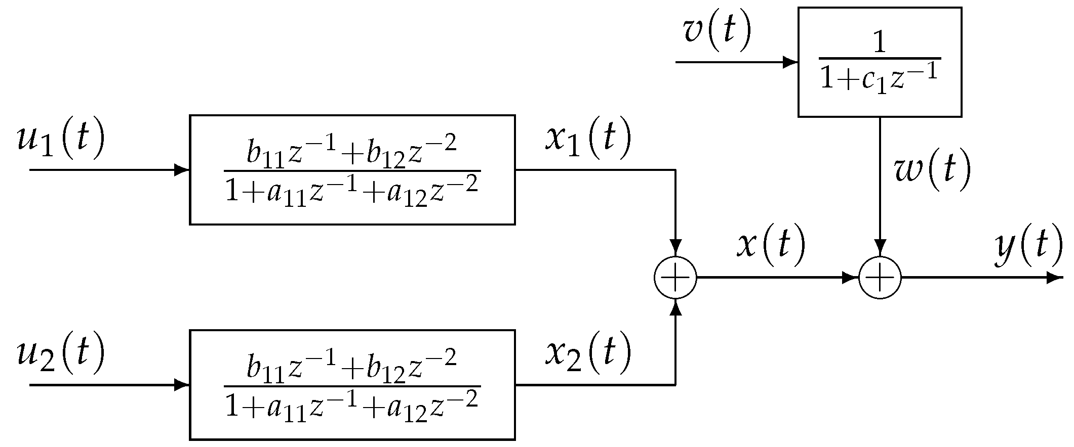
2. The System Description

Consider the following multi-input OEAR system:
x j ( t ) + a j 1 x j ( t 1 ) + a j 2 x j ( t 2 ) + + a j n j x j ( t n j ) = b j 1 u j ( t 1 ) + b j 2 u j ( t 2 ) + + b j n j u j ( t n j ) ,
x ( t ) = j = 1 r x j ( t ) ,
w ( t ) + c 1 w ( t 1 ) + c 2 w ( t 2 ) + + c n c w ( t n c ) = v ( t ) ,
y ( t ) = x ( t ) + w ( t ) ,
where u j ( t ) R , j = 1 , 2 , , r are the inputs, y ( t ) R is the output, x ( t ) R represents the noise-free output, v ( t ) R is random white noise with zero mean, and w ( t ) R is random colored noise. Assume that the orders n j and n c are known, y ( t ) = 0 , u j ( t ) = 0 and v ( t ) = 0 for t 0 . The parameters a j i , b j i and c i are to be identified from input–output data { u j ( t ) , y ( t ) , j = 1 , 2 , , r } .
Define the parameter vectors:
θ : = [ ϑ T , c T ] T R n , n : = n 0 + n c , ϑ : = [ ϑ 1 T , ϑ 2 T , , ϑ r T ] T R n 0 , n 0 : = 2 n 1 + 2 n 2 + + 2 n r , c : = [ c 1 , c 2 , , c n c ] T R n c , ϑ j : = [ a j 1 , a j 2 , , a j n j , b j 1 , b j 2 , , b j n j ] T R 2 n j ,
and the information vectors as
φ ( t ) : = [ ϕ T ( t ) , ψ T ( t ) ] T R n , ϕ ( t ) : = [ ϕ 1 T ( t ) , ϕ 2 T ( t ) , , ϕ r T ( t ) ] T R n 0 , ϕ j ( t ) : = [ x j ( t 1 ) , x j ( t 2 ) , , x j ( t n j ) , u j ( t 1 ) , u j ( t 2 ) , , u j ( t n j ) ] T R 2 n j , ψ ( t ) : = [ w ( t 1 ) , w ( t 2 ) , , w ( t n c ) ] T R n c .
The information vector φ ( t ) is unknown due to the unmeasured variables x j ( t i ) and w ( t i ) . By means of the above definitions, Equations (2)–(4) can be expressed as
x ( t ) = j = 1 r x j ( t ) = j = 1 r ϕ j T ( t ) ϑ j ,
w ( t ) = ψ T ( t ) c + v ( t ) = y ( t ) ϕ T ( t ) ϑ ,
y ( t ) = j = 1 r ϕ j T ( t ) ϑ j + ψ T ( t ) c + v ( t ) = ϕ T ( t ) ϑ + ψ T ( t ) c + v ( t ) = φ T ( t ) θ + v ( t ) .
Equation (7) is the identification model of the multi-input OEAR system, and the parameter vector θ contains all the parameters to be estimated.

3. The Data Filtering Based Recursive Least Squares Algorithm

Define a unit backward shift operator q 1 as q 1 u ( t ) : = u ( t 1 ) and a rational function C ( q ) : = 1 + c 1 q 1 + c 2 q 2 + + c n c q n c . In this section, we use the linear filter C ( q ) to filter the input–output data and derive an F-RGLS algorithm.
For the multi-input OEAR system in Equations (1)–(4), we define the filtered input–output data u j f ( t ) and y f ( t ) as
u j f ( t ) : = C ( q ) u j ( t ) = u j ( t ) + c 1 u j ( t 1 ) + c 2 u j ( t 2 ) + + c n c u j ( t n c ) ,
y f ( t ) : = C ( q ) y ( t ) = y ( t ) + c 1 y ( t 1 ) + c 2 y ( t 2 ) + + c n c y ( t n c ) .
Multiplying both sides of Equations (1) and (4) by C ( q ) , we can obtain the following filtered output-error model:
y f ( t ) = j = 1 r x j f ( t ) + v ( t ) : = x f ( t ) + v ( t ) ,
x j f ( t ) = i = 1 n j a j i x j f ( t i ) + i = 1 n j b j i u j f ( t i ) .
Define the filtered information vectors ϕ f ( t ) and ϕ j f ( t ) as
ϕ f ( t ) : = [ ϕ 1 f T ( t ) , ϕ 2 f T ( t ) , , ϕ r f T ( t ) ] T R n 0 , ϕ j f ( t ) : = [ x j f ( t 1 ) , x j f ( t 2 ) , , x j f ( t n j ) , u j f ( t 1 ) , u j f ( t 2 ) , , u j f ( t n j ) ] T R 2 n j .
Equations (10) and (11) can be rewritten as
x j f ( t ) = ϕ j f T ( t ) ϑ j , y f ( t ) = j = 1 r ϕ j f T ( t ) ϑ j + v ( t )
= ϕ f T ( t ) ϑ + v ( t ) .
Taking advantage of the idea in [28] for the filtered identification model in Equation (13), we can get
ϑ ^ ( t ) = i = 1 t ϕ f ( i ) ϕ f T ( i ) 1 i = 1 t ϕ ( i ) y f ( i ) .
Since the information vector ϕ f ( t ) contains the unknown variables u j f ( t ) and x j f ( t ) , the algorithm in Equation (14) cannot be applied to estimate ϑ ^ ( t ) directly. According to the idea in [29], the unknown variables x j f ( t ) are replaced with the outputs of relevant auxiliary model, and the unmeasurable terms u j f ( t ) and y f ( t ) are replaced with their estimates u ^ j f ( t ) and y ^ f ( t ) , respectively. The derivation process is as follows.
Let ϑ ^ ( t ) , c ^ ( t ) and ϑ ^ j ( t ) be the estimates of ϑ , c and ϑ j at time t, respectively. Use the estimates x ^ j ( t i ) , x ^ j f ( t i ) and u ^ j f ( t i ) to define the estimates of ϕ ( t ) and ϕ f ( t ) as
ϕ ^ ( t ) : = [ ϕ ^ 1 T ( t ) , ϕ ^ 2 T ( t ) , , ϕ ^ r T ( t ) ] T R n 0 , ϕ ^ j ( t ) : = [ x ^ j ( t 1 ) , x ^ j ( t 2 ) , , x ^ j ( t n j ) , u j ( t 1 ) , u j ( t 2 ) , , u j ( t n j ) ] T R 2 n j , ϕ ^ f ( t ) : = [ ϕ ^ 1 f T ( t ) , ϕ ^ 2 f T ( t ) , , ϕ ^ r f T ( t ) ] T R n 0 , ϕ ^ j f ( t ) : = [ x ^ j f ( t 1 ) , x ^ j f ( t 2 ) , , x ^ j f ( t n j ) , u ^ j f ( t 1 ) , u ^ j f ( t 2 ) , , u ^ j f ( t n j ) ] T R 2 n j ,
where the estimates x ^ j ( t ) and x ^ j f ( t ) can be computed by
x ^ j ( t ) = ϕ ^ j T ( t ) ϑ ^ j ( t ) , x ^ j f ( t ) = ϕ ^ j f T ( t ) ϑ ^ j ( t ) .
Define the covariance matrix
P f 1 ( t ) : = i = 1 t ϕ ^ f ( i ) ϕ ^ f T ( i ) = P f 1 ( t 1 ) + ϕ ^ f ( i ) ϕ ^ f T ( i ) ,
and the gain vector
L f ( t ) : = P f ( t ) ϕ ^ f ( t ) .
Equation (14) can be written as
ϑ ^ ( t ) = P f ( t ) i = 1 t ϕ ^ f ( i ) y ^ f ( i ) = P f ( t ) i = 1 t 1 ϕ ^ f ( i ) y ^ f ( i ) + ϕ ^ f ( t ) y ^ f ( t ) = P f ( t ) [ P f 1 ( t 1 ) ϑ ^ ( t 1 ) + ϕ ^ f ( t ) y ^ f ( t ) ] = P f ( t ) [ P f 1 ( t 1 ) ϕ ^ f ( t ) ϕ ^ f T ( t ) ] ϑ ^ ( t 1 ) + P f ( t ) ϕ ^ f ( t ) y ^ f ( t ) = ϑ ^ ( t 1 ) + P f ( t ) ϕ ^ f ( t ) [ y ^ f ( t ) ϕ ^ f T ( t ) ϑ ^ ( t 1 ) ] .
Applying the matrix inversion formula ( A + B C ) 1 = A 1 A 1 B ( I + C A 1 B ) 1 C A 1 to Equation (15), we can obtain the following recursive least squares algorithm for estimating ϑ ^ ( t ) :
ϑ ^ ( t ) = ϑ ^ ( t 1 ) + L f ( t ) [ y f ( t ) ϕ ^ f T ( t ) ϑ ^ ( t 1 ) ] ,
L f ( t ) = P f ( t 1 ) ϕ ^ f ( t ) [ 1 + ϕ ^ f T ( t ) P f ( t 1 ) ϕ ^ f ( t ) ] 1 ,
P f ( t ) = [ I L f ( t ) ϕ ^ f T ( t ) ] P f ( t 1 ) .
Applying the least squares principle to the noise model in Equation (6), we can obtain the following algorithm to estimate the parameter vector c:
c ^ ( t ) = c ^ ( t 1 ) + L n ( t ) [ w ( t ) ψ T ( t ) c ( t 1 ) ] ,
L n ( t ) = P n ( t 1 ) ψ ( t ) [ 1 + ψ T ( t ) P n ( t 1 ) ψ ( t ) ] 1 ,
P n ( t ) = [ I L n ( t ) ψ T ( t ) ] P n ( t 1 ) .
The noise information vector ψ ( t ) involves the unknown term w ( t i ) . From Equations (6) and (7), once the estimate ϑ ^ ( t ) is obtained, the estimate w ^ ( t ) can be computed by
w ^ ( t ) = y ( t ) ϕ ^ T ( t ) ϑ ^ ( t 1 ) .
Replace the unmeasurable noise terms w ( t i ) in ψ ( t ) with estimates w ^ ( t i ) and define the estimate of ψ ( t ) as
ψ ^ ( t ) : = [ w ^ ( t 1 ) , w ^ ( t 2 ) , , w ^ ( t n c ) ] R n c .
Use the estimate c ^ ( t ) : = [ c ^ 1 ( t ) , c ^ 2 ( t ) , , c ^ n c ( t ) ] T R n c to form the estimate of C ( q ) as follows:
C ^ ( t , q ) : = 1 + c ^ 1 ( t ) q 1 + c ^ 2 ( t ) q 2 + + c ^ n c ( t ) q n c .
The estimates of the filtered input u j f ( t ) and the filtered output y f ( t ) can be computed through
u ^ j f ( t ) = C ^ ( t , q ) u j ( t ) = u j ( t ) + [ u j ( t 1 ) , u j ( t 2 ) , , u j ( t n c ) ] c ^ ( t ) , y ^ f ( t ) = C ^ ( t , q ) y ( t ) = y ( t ) + [ y ( t 1 ) , y ( t 2 ) , , y ( t n c ) ] c ^ ( t ) .
Replacing ϕ f ( t ) and y f ( t ) in Equations (16)–(18) with their estimates ϕ ^ f ( t ) and y ^ f ( t ) , and replacing ψ ( t ) and w ( t ) in Equations (19)–(21) with their estimates ψ ^ ( t ) and w ^ ( t ) , we can summarize the data filtering based recursive generalized least squares (F-RGLS) algorithm for the multi-input OEAR systems:
ϑ ^ ( t ) = ϑ ^ ( t 1 ) + L f ( t ) [ y ^ f ( t ) ϕ ^ f T ( t ) ϑ ^ ( t 1 ) ] ,
L f ( t ) = P f ( t 1 ) ϕ ^ f ( t ) [ 1 + ϕ ^ f T ( t ) P f ( t 1 ) ϕ ^ f ( t ) ] 1 ,
P f ( t ) = [ I L f ( t ) ϕ ^ f T ( t ) ] P f ( t 1 ) ,
x ^ j f ( t ) = ϕ ^ j f T ( t ) ϑ ^ j ( t ) ,
ϕ ^ f ( t ) = [ ϕ ^ 1 f T ( t ) , ϕ ^ 2 f T ( t ) , , ϕ ^ r f T ( t ) ] T ,
ϕ ^ j f ( t ) = [ x ^ j f ( t 1 ) , x ^ j f ( t 2 ) , , x ^ j f ( t n j ) , u ^ j f ( t 1 ) , u ^ j f ( t 2 ) , , u ^ j f ( t n j ) ] T ,
u ^ j f ( t ) = u j ( t ) + c ^ 1 ( t ) u j ( t 1 ) + c ^ 2 ( t ) u j ( t 2 ) + + c ^ n c ( t ) u j ( t n c ) ,
y ^ f ( t ) = y ( t ) + c ^ 1 ( t ) y ( t 1 ) + c ^ 2 ( t ) y ( t 2 ) + + c ^ n c ( t ) y ( t n c ) ,
c ^ ( t ) = c ^ ( t 1 ) + L n ( t ) [ w ^ ( t ) ψ ^ T ( t ) c ^ ( t 1 ) ] ,
L n ( t ) = P n ( t 1 ) ψ ^ ( t ) [ 1 + ψ ^ T ( t ) P n ( t 1 ) ψ ^ ( t ) ] 1 ,
P n ( t ) = [ I L n ( t ) ψ ^ T ( t ) ] P n ( t 1 ) ,
w ^ ( t ) = y ( t ) ϕ ^ T ( t ) ϑ ^ ( t 1 ) ,
x ^ j ( t ) = ϕ ^ j T ( t ) ϑ ^ j ( t ) ,
ϕ ^ ( t ) = [ ϕ ^ 1 T ( t ) , ϕ ^ 2 T ( t ) , , ϕ ^ r T ( t ) ] T ,
ϕ ^ j ( t ) = [ x ^ j ( t 1 ) , x ^ j ( t 2 ) , , x ^ j ( t n j ) , u j ( t 1 ) , u j ( t 2 ) , , u j ( t n j ) ] T ,
ψ ^ ( t ) = [ w ^ ( t 1 ) , w ^ ( t 2 ) , , w ^ ( t n c ) ] T ,
ϑ ^ ( t ) = [ ϑ ^ 1 T ( t ) , ϑ ^ 2 T ( t ) , , ϑ ^ r T ( t ) ] T ,
ϑ ^ j ( t ) = [ a ^ j 1 ( t ) , a ^ j 2 ( t ) , , a ^ j n j ( t ) , b ^ j 1 ( t ) , b ^ j 2 ( t ) , , b ^ j n j ( t ) ] T ,
c ^ ( t ) = [ c ^ 1 ( t ) , c ^ 2 ( t ) , , c ^ n c ( t ) ] T .
The F-RGLS estimation algorithm involves two steps: the parameter identification of the system model—see Equations (22)–(29)—and the parameter identification of the noise model—see Equations (30)–(37). The F-RGLS algorithm can generate the parameter estimation of the multi-input OEAR system; however, the algorithm uses only the measured data { u j ( i ) , y ( i ) : i = 0 , 1 , 2 , , t } up to time t, not including the data { u ( i ) , y ( i ) : i = t + 1 , t + 2 , , L } . Next, we will make full use of all the measured data to improve the parameter estimation accuracy by adopting the iterative identification approach.

4. The Data Filtering Based Iterative Least Squares Algorithm

Suppose that the data length L n 0 + n c . Based on the identification models in Equations (6) and (13), we define two quadratic criterion functions
J 1 ( ϑ ) : = t = 1 L [ y f ( t ) ϕ f T ( t ) ϑ ] 2 , J 2 ( c ) : = t = 1 L [ w ( t ) ψ T ( t ) c ] 2 .
Minimizing the above two quadratic criterion functions, we can obtain the estimation algorithm of computing ϑ ^ ( t ) and c ^ ( t ) :
ϑ ^ ( t ) = t = 1 L ϕ f ( t ) ϕ f T ( t ) 1 t = 1 L ϕ f ( t ) y f ( t ) ,
c ^ ( t ) = t = 1 L ψ ( t ) ψ T ( t ) 1 t = 1 L ψ ( t ) w ( t ) .
Because the vectors ϕ f ( t ) and ψ ( t ) are unknown, the parameter estimates ϑ ^ ( t ) and c ^ ( t ) cannot be computed directly. Here, we adopt the iterative estimation theory. Let k = 1 , 2 , 3 , be an iterative variable, ϑ ^ k and c ^ k denote the iterative estimates of ϑ and c at iteration k. Let x ^ j , k ( t ) and w ^ k ( t ) be the estimates of x j ( t ) and w ( t ) at iteration k. Replacing ϕ j ( t ) and ϑ j in Equation (5) with their estimates ϕ ^ j , k ( t ) and ϑ ^ j , k at iteration k, ϕ ( t ) and ϑ in Equation (6) with their estimates ϕ ^ k ( t ) at iteration k and the ϑ ^ k 1 at iteration k 1 , the estimate x ^ j , k ( t ) and w ^ k ( t ) can be calculated by
x ^ j , k ( t ) = ϕ ^ j , k T ( t ) ϑ ^ j , k ,
w ^ k ( t ) = y ( t ) ϕ ^ k T ( t ) ϑ ^ k 1 .
Replacing x j ( t i ) in ϕ j ( t ) with x ^ j , k 1 ( t i ) , w ( t i ) in ψ ( t ) with w ^ k 1 ( t i ) , the estimates ϕ ^ k ( t ) , ϕ ^ j , k ( t ) and ψ ^ k ( t ) can be obtained by
ϕ ^ k ( t ) = [ ϕ ^ 1 , k T ( t ) , ϕ ^ 2 , k T ( t ) , , ϕ ^ r , k T ( t ) ] T ,
ϕ ^ j , k ( t ) = [ x ^ j , k 1 ( t 1 ) , , x ^ j , k 1 ( t n j ) , u j ( t 1 ) , , u j ( t n j ) ] T ,
ψ ^ k ( t ) = [ w ^ k 1 ( t 1 ) , w ^ k 1 ( t 2 ) , , w ^ k 1 ( t n c ) ] T .
Using the parameter estimate c ^ k = [ c ^ 1 , k , c ^ 2 , k , , c ^ n c , k ] T to form the estimate of C ( q ) at iteration k:
C ^ k ( q ) : = 1 + c ^ 1 , k q 1 + c ^ 2 , k q 2 + + c ^ n c , k q n c .
Filtering the input–output data u j ( t ) and y ( t ) by C ^ k ( q ) , we can obtain the estimates of u j f ( t ) and y f ( t )
u ^ j f , k ( t ) = C ^ k ( q ) u j ( t ) = u j ( t ) + [ u j ( t 1 ) , u j ( t 2 ) , , u j ( t n c ) ] c ^ k ,
y ^ f , k ( t ) = C ^ k ( q ) y ( t ) = y ( t ) + [ y ( t 1 ) , y ( t 2 ) , , y ( t n c ) ] c ^ k .
Let x ^ j f , k ( t ) be the estimate of x j f ( t ) at iteration k, replacing ϕ j f ( t ) and ϑ j in Equation (12) with their estimates ϕ ^ j f , k ( t ) and ϑ ^ j , k at iteration k, the estimate x ^ j f , k ( t ) can be computed by
x ^ j f , k ( t ) = ϕ ^ j f , k T ( t ) ϑ ^ j , k .
Replacing x j f ( t i ) and u j f ( t i ) in ϕ j f ( t ) with their estimates x ^ j f , k 1 ( t i ) at iteration k 1 and u ^ j f , k ( t i ) at iteration k, we can obtain the estimates:
ϕ ^ f , k ( t ) = [ ϕ ^ 1 f , k T ( t ) , ϕ ^ 2 f , k T ( t ) , , ϕ ^ r f , k T ( t ) ] T ,
ϕ ^ j f , k ( t ) = [ x ^ j f , k 1 ( t 1 ) , , x ^ j f , k 1 ( t n j ) , u ^ j f , k ( t 1 ) , , u ^ j f , k ( t n j ) ] T .
Replacing ϕ f ( t ) and y f ( t ) in Equation (41) with their estimates ϕ ^ f , k ( t ) and y ^ f , k ( t ) , and replacing ψ ( t ) and w ( t ) in Equation (42) with their estimates ψ ^ k ( t ) and w ^ k ( t ) , we can obtain the data filtering based iterative least squares (F-LSI) algorithm of estimating the parameter vectors ϑ and c:
ϑ ^ k = t = 1 L ϕ ^ f , k ( t ) ϕ ^ f , k T ( t ) 1 t = 1 L ϕ ^ f , k ( t ) y ^ f , k ( t ) , k = 1 , 2 , 3 ,
c ^ k = t = 1 L ψ ^ k ( t ) ψ ^ k T ( t ) 1 t = 1 L ψ ^ k ( t ) w ^ k ( t ) .
From Equations (43)–(54), we can summarize the F-LSI algorithm as follows:
ϑ ^ k = t = 1 L ϕ ^ f , k ( t ) ϕ ^ f , k T ( t ) 1 t = 1 L ϕ ^ f , k ( t ) y ^ f , k ( t ) , k = 1 , 2 , 3 ,
ϕ ^ f , k ( t ) = [ ϕ ^ 1 f , k T ( t ) , ϕ ^ 2 f , k T ( t ) , , ϕ ^ r f , k T ( t ) ] T ,
ϕ ^ j f , k ( t ) = [ x ^ j f , k 1 ( t 1 ) , , x ^ j f , k 1 ( t n j ) , u ^ j f , k ( t 1 ) , , u ^ j f , k ( t n j ) ] T ,
u ^ j f , k ( t ) = u j ( t ) + c ^ 1 , k u j ( t 1 ) + c ^ 2 , k u j ( t 2 ) + + c ^ n c , k u j ( t n c ) ,
y ^ f , k ( t ) = y ( t ) + c ^ 1 , k y ( t 1 ) + c ^ 2 , k y ( t 2 ) + + c ^ n c , k y ( t n c ) ,
x ^ j f , k ( t ) = ϕ ^ j f , k T ( t ) ϑ ^ j , k ,
c ^ k = t = 1 L ψ ^ k ( t ) ψ ^ k T ( t ) 1 t = 1 L ψ ^ k ( t ) w ^ k ( t ) ,
ψ ^ k ( t ) = [ w ^ k 1 ( t 1 ) , w ^ k 1 ( t 2 ) , , w ^ k 1 ( t n c ) ] T ,
ϕ ^ k ( t ) = [ ϕ ^ 1 , k T ( t ) , ϕ ^ 2 , k T ( t ) , , ϕ ^ r , k T ( t ) ] T ,
ϕ ^ j , k ( t ) = [ x ^ j , k 1 ( t 1 ) , , x ^ j , k 1 ( t n j ) , u j ( t 1 ) , , u j ( t n j ) ] T ,
x ^ j , k ( t ) = ϕ ^ j , k T ( t ) ϑ ^ j , k ,
w ^ k ( t ) = y ( t ) ϕ ^ k T ( t ) ϑ ^ k 1 ,
ϑ ^ k = [ ϑ ^ 1 , k T , ϑ ^ 2 , k T , , ϑ ^ r , k T ] T ,
ϑ ^ j , k = [ a ^ j 1 , k , a ^ j 2 , k , , a ^ j n j , k , b ^ j 1 , k , b ^ j 2 , k , , b ^ j n j , k ] T ,
c ^ k = [ c ^ 1 , k , c ^ 2 , k , , c ^ n c , k ] T .
We list the steps for computing the estimates ϑ ^ k and c ^ k as iteration k increases:
  • To initialize, let k = 1 , x ^ j f , 0 ( t ) = 1 / p 0 , u ^ j f , 0 ( t ) = 1 / p 0 , y ^ f , 0 ( t ) = 1 / p 0 , x ^ j , 0 ( t ) = 1 / p 0 , w ^ 0 ( t ) = 1 / p 0 , p 0 = 10 6 .
  • Collect the input–output data { u 1 ( t ) , u 2 ( t ) , , u r ( t ) , y ( t ) : t = 1 , 2 , , L } .
  • Form ϕ ^ j , k ( t ) by Equation (64), ϕ ^ k ( t ) by Equation (63), and ψ ^ k ( t ) by Equation (62).
  • Compute w ^ k ( t ) by Equation (66), update the parameter estimate c ^ k by Equation (61).
  • Read c ^ k by Equation (69), compute u ^ j f , k ( t ) and y ^ f , k ( t ) by Equations (58) and (59).
  • Form ϕ ^ f , k ( t ) and ϕ ^ j f , k ( t ) by Equations (56) and (57), update the parameter estimate ϑ ^ k by Equation (55).
  • Read ϑ ^ j , k by Equation (68), compute x ^ j f , k ( t ) and x ^ j , k ( t ) by Equations (60) and (65).
  • Give a small positive ε, compare θ ^ k = ϑ ^ k c ^ k with θ ^ k 1 , if θ ^ k θ ^ k 1 ε , obtain the iterative time k and the parameter estimate θ ^ k , increase k by 1 and go to Step 2; otherwise, increase k by 1 and go to Step 3.
Remark
The computational complexity implies the computational amount of multiplications and adds in the algorithm, depending on the sizes and lengths.

5. Examples

Example 1
Consider the following multi-input OEAR system:
x 1 ( t ) + a 11 x 1 ( t 1 ) + a 12 x 1 ( t 2 ) = b 11 u 1 ( t 1 ) + b 12 u 1 ( t 2 ) ,
x 2 ( t ) + a 21 x 2 ( t 1 ) + a 22 x 2 ( t 2 ) = b 21 u 2 ( t 1 ) + b 22 u 2 ( t 2 ) ,
w ( t ) + c 1 w ( t 1 ) = v ( t ) ,
y ( t ) = x 1 ( t ) + x 2 ( t ) + w ( t ) .
The parameter vector to be estimated is
θ = [ a 11 , a 12 , b 11 , b 12 , a 21 , a 22 , b 21 , b 22 , c 1 ] T = [ 0 . 15 , 0 . 25 , 0 . 99 , 0 . 78 , 0 . 10 , 0 . 35 , 0 . 50 , 0 . 80 , 0 . 20 ] T .
The inputs { u 1 ( t ) , u 2 ( t ) } are taken as two persistent excitation signal sequences with zero mean and unit variance, and { v ( t ) } as a white noise sequence with zero mean and variance σ 2 = 0 . 20 2 and σ 2 = 0 . 60 2 .
Applying the F-RGLS algorithm to estimate the parameters of this example system, the parameter estimates and their estimation errors δ : = θ ^ ( t ) θ / θ are shown in Table 1. Applying the F-LSI algorithm to estimate the parameters of this example system, when the data length L = 2000 the parameter estimates and their estimation errors δ : = θ ^ k θ / θ are shown in Table 2 with different noise variances. When the data length L = 4000 , the parameter estimates and their errors δ are shown in Table 3 with different noise variances. Under different noise variances and different data lengths, the parameter estimates and their errors δ are shown in Table 4 when the iteration k = 10 . Under different noise variances, the parameter estimation errors δ versus k are shown in Figure 1.
From Table 1, Table 2, Table 3 and Table 4 and Figure 1, we can draw the following conclusions:
  • Increasing the data length L can improve the parameter estimation accuracy of the F-RGLS algorithm and the F-LSI algorithm, and as the data length L increases, the parameter estimates are getting more stationary.
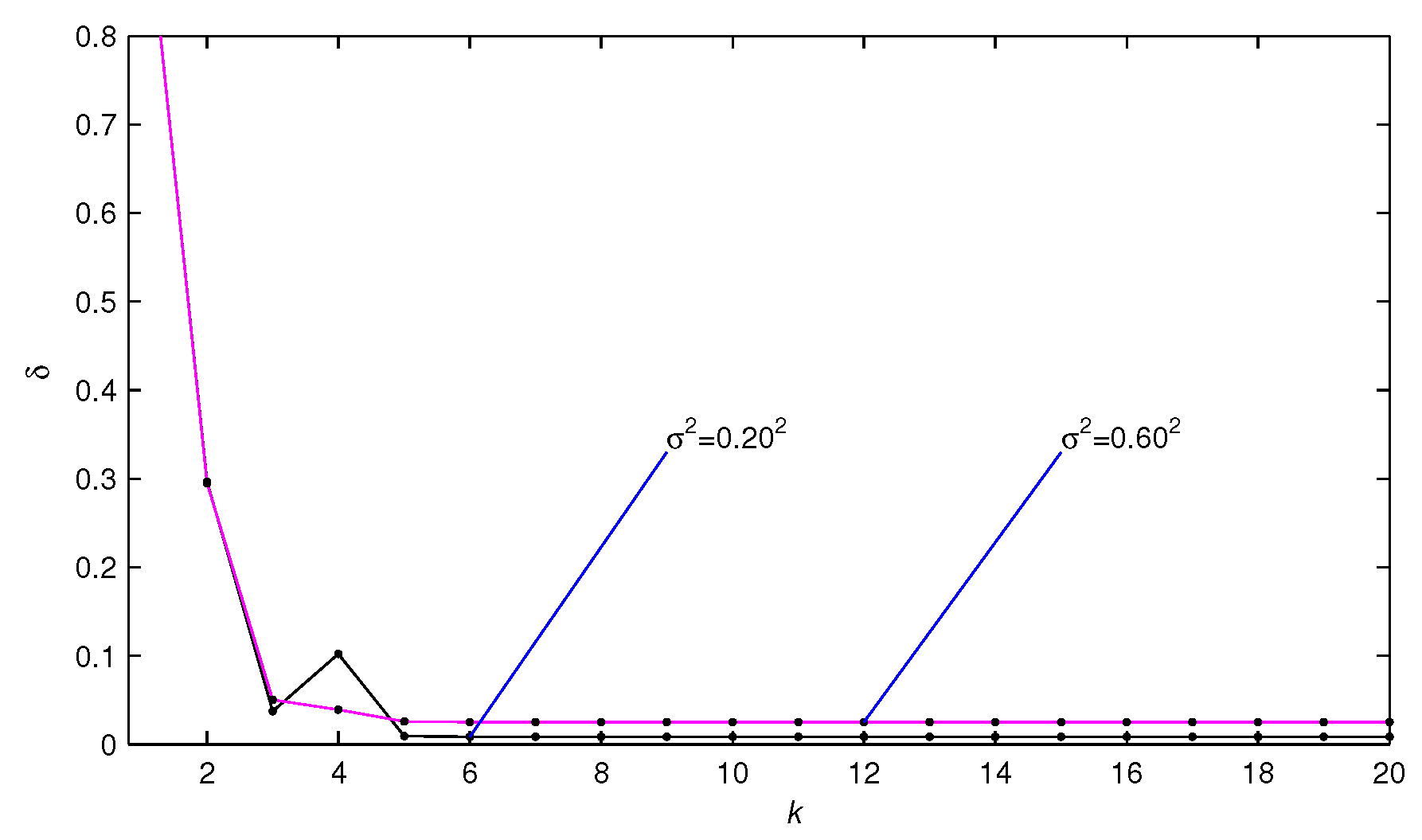
  • Under the same data length, the estimation accuracy of the F-RGLS algorithm and the F-LSI algorithm increases as the noise variance decreases.
  • Under the same data length and noise variance, the estimation errors of the F-LSI algorithm are smaller than the F-RGLS algorithm.
  • The F-LSI algorithm has fast convergence speed, and the parameter estimates only need several iterations close to their true values.
Example 2
Consider the industrial process with colored noise, which has two inputs and one output as shown in Figure 2 and described as
y ( t ) = G 1 ( z ) u 1 ( t ) + G 2 ( z ) u 2 ( t ) + H ( z ) v ( t ) = i = 1 2 [ a 1 i x 1 ( t i ) + b 1 i u 1 ( t i ) ] + i = 1 2 [ a 2 i x 2 ( t i ) + b 2 i u 2 ( t i ) ] c 1 w ( t 1 ) + v ( t ) ,
where G 1 ( z ) = ( b 11 z 1 + b 12 z 2 ) / ( 1 + a 11 z 1 + a 12 z 2 ) , G 2 ( z ) = ( b 21 z 1 + b 22 z 2 ) / ( 1 + a 21 z 1 + a 22 z 2 ) and H ( z ) = 1 / ( 1 + c 1 z 1 ) .
The parameters to be estimated are
[ a 11 , a 12 , b 11 , b 12 , a 21 , a 22 , b 21 , b 22 , c 1 ] T = [ 0 . 15 , 0 . 25 , 0 . 99 , 0 . 78 , 0 . 10 , 0 . 35 , 0 . 50 , 0 . 80 , 0 . 20 ] T .
The simulation conditions are the same as those of Example 1, and the noise variance σ 2 = 0 . 30 2 . Applying the F-RGLS and the F-LSI algorithms to estimate the parameters of the system, the parameter estimates and their errors are presented in Table 5 and Table 6.
From Table 5 and Table 6, we can see that the estimation errors become smaller with the increase of t and the F-LSI algorithm can get accurate parameter estimates by only several iterations, which shows the effectiveness of the proposed algorithms.
The power consumption in host servers can be concerned by the model of Example 2. The two inputs are the changes in CPU frequency of the host server and the changes in the guest server’s time share to use the physical CPU of the host server, and the power consumption is the system output. The configuration and the allocation of memory, storage and network bandwidth for the guest server are the random disturbances of the system.

6. Conclusions

This paper discusses the parameter estimation problem for multi-input OEAR systems. Based on the data filtering technique, an F-RGLS algorithm and an F-LSI algorithm are developed. The proposed methods are effective for estimating the parameters of multi-input OEAR systems. The simulation results indicate that the proposed F-LSI algorithm achieves higher estimation accuracies than the F-RGLS algorithm, and the convergence rate of the proposed methods can be improved by increasing the data length. The methods used in this paper can be extended to study the identification of other linear systems, nonlinear systems, state space systems and time delay systems.

Acknowledgments

This work was supported by the Visiting Scholar Project for Young Backbone Teachers of Shandong Province, China.

Conflicts of Interest

The author declares no conflict of interest.

References

  1. Mobayen, S. An LMI-based robust tracker for uncertain linear systems with multiple time-varying delays using optimal composite nonlinear feedback technique. Nonlinear Dyn. 2015, 80, 917–927. [Google Scholar] [CrossRef]
  2. Saab, S.S.; Toukhtarian, R. A MIMO sampling-rate-dependent controller. IEEE Trans. Ind. Electron. 2015, 62, 3662–3671. [Google Scholar] [CrossRef]
  3. Garnier, H.; Gilson, M.; Young, P.C.; Huselstein, E. An optimal iv technique for identifying continuous-time transfer function model of multiple input systems. Control Eng. Pract. 2007, 46, 471–486. [Google Scholar] [CrossRef]
  4. Chouaba, S.E.; Chamroo, A.; Ouvrard, R.; Poinot, T. A counter flow water to oil heat exchanger: MISO quasi linear parameter varying modeling and identification. Simulat. Model. Pract. Theory 2012, 23, 87–98. [Google Scholar] [CrossRef]
  5. Halaoui, M.E.; Kaabal, A.; Asselman, H.; Ahyoud, S.; Asselman, A. Dual band PIFA for WLAN and WiMAX MIMO systems for mobile handsets. Procedia Technol. 2016, 22, 878–883. [Google Scholar] [CrossRef]
  6. Al-Hazemi, F.; Peng, Y.Y.; Youn, C.H. A MISO model for power consumption in virtualized servers. Cluster Comput. 2015, 18, 847–863. [Google Scholar] [CrossRef]
  7. Yerramilli, S.; Tangirala, A.K. Detection and diagnosis of model-plant mismatch in MIMO systems using plant-model ratio. IFAC-Papers OnLine 2016, 49, 266–271. [Google Scholar] [CrossRef]
  8. Sannuti, P.; Saberi, A.; Zhang, M.R. Squaring down of general MIMO systems to invertible uniform rank systems via pre- and/or post- compensators. Automatica 2014, 50, 2136–2141. [Google Scholar] [CrossRef]
  9. Wang, Y.J.; Ding, F. Novel data filtering based parameter identification for multiple-input multiple-output systems using the auxiliary model. Automatica 2016, 71, 308–313. [Google Scholar] [CrossRef]
  10. Wang, D.Q.; Ding, F. Parameter estimation algorithms for multivariable Hammerstein CARMA systems. Inf. Sci. 2016, 355, 237–248. [Google Scholar] [CrossRef]
  11. Liu, Y.J.; Tao, T.Y. A CS recovery algorithm for model and time delay identification of MISO-FIR systems. Algorithms 2015, 8, 743–753. [Google Scholar] [CrossRef]
  12. Wang, X.H.; Ding, F. Convergence of the recursive identification algorithms for multivariate pseudo-linear regressive systems. Int. J. Adapt. Control Signal Process. 2016, 30, 824–842. [Google Scholar] [CrossRef]
  13. Ji, Y.; Liu, X.M. Unified synchronization criteria for hybrid switching-impulsive dynamical networks. Circuits Syst. Signal Process. 2015, 34, 1499–1517. [Google Scholar] [CrossRef]
  14. Meng, D.D.; Ding, F. Model equivalence-based identification algorithm for equation-error systems with colored noise. Algorithms 2015, 8, 280–291. [Google Scholar] [CrossRef]
  15. Wang, Y.J.; Ding, F. The filtering based iterative identification for multivariable systems. IET Control Theory Appl. 2016, 10, 894–902. [Google Scholar] [CrossRef]
  16. Dehghan, M.; Hajarian, M. Finite iterative methods for solving systems of linear matrix equations over reflexive and anti-reflexive matrices. Bull. Iran. Math. Soc. 2014, 40, 295–323. [Google Scholar]
  17. Xu, L. The damping iterative parameter identification method for dynamical systems based on the sine signal measurement. Signal Process. 2016, 120, 660–667. [Google Scholar] [CrossRef]
  18. Zhang, W.G. Decomposition based least squares iterative estimation for output error moving average systems. Eng. Comput. 2014, 31, 709–725. [Google Scholar] [CrossRef]
  19. Zhou, L.C.; Li, X.L.; Xu, H.G.; Zhu, P.Y. Gradient-based iterative identification for Wiener nonlinear dynamic systems with moving average noises. Algorithms 2015, 8, 712–722. [Google Scholar] [CrossRef]
  20. Shi, P.; Luan, X.L.; Liu, F. H-infinity filtering for discrete-time systems with stochastic incomplete measurement and mixed delays. IEEE Trans. Ind. Electron. 2012, 59, 2732–2739. [Google Scholar] [CrossRef]
  21. Wang, Y.J.; Ding, F. The auxiliary model based hierarchical gradient algorithms and convergence analysis using the filtering technique. Signal Process. 2016, 128, 212–221. [Google Scholar] [CrossRef]
  22. Li, X.Y.; Sun, S.L. H-infinity filtering for networked linear systems with multiple packet dropouts and random delays. Digital Signal Process. 2015, 46, 59–67. [Google Scholar] [CrossRef]
  23. Ding, F.; Liu, X.M.; Gu, Y. An auxiliary model based least squares algorithm for a dual-rate state space system with time-delay using the data filtering. J. Franklin Inst. 2016, 353, 398–408. [Google Scholar] [CrossRef]
  24. Zhang, L.; Wang, Z.P.; Sun, F.C.; Dorrell, D.G. Online parameter identification of ultracapacitor models using the extended kalman filter. Algorithms 2014, 7, 3204–3217. [Google Scholar] [CrossRef]
  25. Basin, M.; Shi, P.; Calderon-Alvarez, D. Joint state filtering and parameter estimation for linear stochastic time-delay systems. Signal Process. 2011, 91, 782–792. [Google Scholar] [CrossRef]
  26. Scarpiniti, M.; Comminiello, D.; Parisi, R.; Uncini, A. Nonlinear system identification using IIR Spline Adaptive filters. Signal Process. 2015, 108, 30–35. [Google Scholar] [CrossRef]
  27. Wang, C.; Tang, T. Several gradient-based iterative estimation algorithms for a class of nonlinear systems using the filtering technique. Nonlinear Dyn. 2014, 77, 769–780. [Google Scholar] [CrossRef]
  28. Ding, F.; Wang, Y.J.; Ding, J. Recursive least squares parameter identification for systems with colored noise using the filtering technique and the auxiliary model. Digital Signal Process. 2015, 37, 100–108. [Google Scholar] [CrossRef]
  29. Wang, D.Q. Least squares-based recursive and iterative estimation for output error moving average systems using data filtering. IET Control Theory Appl. 2011, 5, 1648–1657. [Google Scholar] [CrossRef]
Figure 1. The estimation errors δ versus t.
Algorithms 09 00049 g001
Figure 2. The diagram of a multi-input OEAR system.
Algorithms 09 00049 g002
Table 1. The F-RGLS estimates and their errors for Example 1.
σ 2 t = L a 11 a 12 b 11 b 12 a 21 a 22 b 21 b 22 c 1 δ ( % )
0 . 20 2 1000.142400.234940.96900−0.75613−0.110710.35200−0.51875−0.807340.0030212.18486
2000.145790.250050.96382−0.78341−0.101890.35013−0.49750−0.789420.110455.68913
5000.152220.263640.97647−0.77308−0.090600.35005−0.48724−0.788570.132624.41957
10000.158920.259700.98546−0.76410−0.100050.34897−0.49297−0.785590.152573.28600
20000.154430.258200.98663−0.77005−0.102140.34954−0.49407−0.795320.155692.85038
30000.153180.259790.99026−0.77528−0.100250.35272−0.49559−0.799630.158302.63155
0 . 60 2 1000.166610.220880.97687−0.76637−0.047960.28133−0.58256−0.92613−0.0107716.67281
2000.142300.247040.95213−0.83607−0.061330.30376−0.51120−0.824060.109777.91161
5000.151810.281540.96971−0.78348−0.060340.33148−0.46893−0.785590.144725.25893
10000.171420.271610.98894−0.74692−0.090930.33498−0.48227−0.769100.157224.45410
20000.161540.270690.98704−0.75643−0.100490.34152−0.48438−0.793060.161093.31329
30000.158470.276330.99597−0.76992−0.096640.35335−0.48844−0.803720.163762.95257
True values0.150000.250000.99000−0.78000−0.100000.35000−0.50000−0.800000.20000
Table 2. The F-LSI parameter estimates and errors for Example 1 ( L = 2000 ).
σ 2 k a 11 a 12 b 11 b 12 a 21 a 22 b 21 b 22 c 1 δ ( % )
0 . 20 2 1−0.02217−0.027410.000000.000000.000000.000000.000000.00000−0.04161100.72791
20.000000.000000.97952−0.910910.000000.00000−0.49792−0.864780.1585829.65842
50.156010.257970.98928−0.77078−0.099370.34653−0.49427−0.798730.198110.92811
100.155190.257270.98927−0.77191−0.099930.34719−0.49479−0.798100.202070.83049
0 . 60 2 1−0.02217−0.027410.000000.000000.000000.000000.000000.00000−0.04161100.72791
20.000000.000000.97808−0.903540.000000.00000−0.48514−0.860830.1644029.49952
50.166530.272480.98778−0.75450−0.099140.34084−0.48385−0.795050.201212.56878
100.165960.271940.98782−0.75539−0.099860.34146−0.48438−0.794260.202092.49317
True values0.150000.250000.99000−0.78000−0.100000.35000−0.50000−0.800000.20000
Table 3. The F-LSI parameter estimates and errors for Example 1 ( L = 4000 ).
σ 2 k a 11 a 12 b 11 b 12 a 21 a 22 b 21 b 22 c 1 δ ( % )
0 . 20 2 1−0.00166−0.026860.000000.000000.000000.000000.000000.00000−0.04216100.60660
20.000000.000000.98621−0.918560.000000.00000−0.50246−0.861960.1605629.74749
50.153070.259030.99062−0.77955−0.098660.34570−0.49802−0.801450.189880.89726
100.152390.258450.99072−0.78046−0.099640.34658−0.49821−0.800510.192380.74333
0 . 60 2 1−0.00166−0.026860.000000.000000.000000.000000.000000.00000−0.04216100.60660
20.000000.000000.98710−0.923160.000000.00000−0.49770−0.864260.1630129.83299
50.157760.275650.99202−0.78054−0.097570.33874−0.49436−0.802780.191631.87793
100.157080.275010.99217−0.78149−0.098820.33965−0.49462−0.801600.192401.79377
True values0.150000.250000.99000−0.78000−0.100000.35000−0.50000−0.800000.20000
Table 4. The F-LSI parameter estimates and errors for Example 1 ( k = 10 ).
σ 2 L a 11 a 12 b 11 b 12 a 21 a 22 b 21 b 22 c 1 δ ( % )
0 . 20 2 20000.155190.257270.98927−0.77191−0.099930.34719−0.49479−0.798100.202070.83049
40000.152390.258450.99072−0.78046−0.099640.34658−0.49821−0.800510.192380.74333
0 . 60 2 20000.165960.271940.98782−0.75539−0.099860.34146−0.48438−0.794260.202092.49317
40000.157080.275010.99217−0.78149−0.098820.33965−0.49462−0.801600.192401.79377
True values0.150000.250000.99000−0.78000−0.100000.35000−0.50000−0.800000.20000
Table 5. The F-RGLS parameter estimates and errors for Example 2.
t a 11 a 12 b 11 b 12 a 21 a 22 b 21 b 22 c 1 δ ( % )
1000.310440.273230.478230.79593−0.169880.312330.347330.79082−0.3599011.48781
2000.357120.261070.475340.80554−0.201880.328070.384680.77922−0.304697.07660
5000.375580.303330.484850.83653−0.221430.300580.412460.78396−0.286694.56000
10000.360220.291640.496900.84216−0.230720.291990.405190.76406−0.271382.49100
20000.361150.295400.497710.84667−0.240940.300370.399380.74612−0.274342.05076
30000.366360.301390.502630.84719−0.243890.306500.396580.74012−0.265541.89797
True values0.350000.300000.500000.84000−0.250000.300000.400000.75000−0.25000
Table 6. The F-LSI parameter estimates and errors for Example 2.
k a 11 a 12 b 11 b 12 a 21 a 22 b 21 b 22 c 1 δ ( % )
1−0.006110.036010.000000.000000.000000.000000.000000.000000.0016599.63926
20.000000.000000.499600.677160.000000.000000.410140.84617−0.2645243.64422
30.485120.143790.507750.90619−0.223590.259260.399840.75210−0.2645215.35917
40.352310.336450.504640.84218−0.251810.317250.398040.73802−0.1038510.48969
50.359680.294430.502700.84889−0.248230.312430.398310.73841−0.0416214.44370
60.364740.297710.503050.84987−0.249110.313580.398190.73823−0.249511.76580
70.363360.299240.503260.84956−0.248690.312890.398080.73850−0.256961.73424
80.363280.298610.503270.84966−0.248680.312860.398090.73855−0.256981.73382
90.363360.298620.503270.84967−0.248650.312860.398080.73856−0.257031.73724
100.363350.298640.503270.84966−0.248650.312850.398080.73856−0.257021.73638
True values0.350000.300000.500000.84000−0.250000.300000.400000.75000−0.25000

