Utilizing Network Structure to Accelerate Markov Chain Monte Carlo Algorithms

Abstract

We consider the problem of estimating the measure of subsets in very large networks. A prime tool for this purpose is the Markov Chain Monte Carlo (MCMC) algorithm. This algorithm, while extremely useful in many cases, still often suffers from the drawback of very slow convergence. We show that in a special, but important case, it is possible to obtain significantly better bounds on the convergence rate. This special case is when the huge state space can be aggregated into a smaller number of clusters, in which the states behave approximately the same way (but their behavior still may not be identical). A Markov chain with this structure is called quasi-lumpable. This property allows the aggregation of states (nodes) into clusters. Our main contribution is a rigorously proved bound on the rate at which the aggregated state distribution approaches its limit in quasi-lumpable Markov chains. We also demonstrate numerically that in certain cases this can indeed lead to a significantly accelerated way of estimating the measure of subsets. The result can be a useful tool in the analysis of complex networks, whenever they have a clustering that aggregates nodes with similar (but not necessarily identical) behavior.

1. Introduction

The Markov Chain Monte Carlo (MCMC) method is one of the most frequently used algorithms to solve hard counting, sampling and optimization problems. This is relevant for many areas, including complex networks, physics, communication systems, computational biology, optimization, data mining, big data analysis, forecast problems, prediction tasks, and innumerable others. The success and influence of the method is shown by the fact that it has been selected as one of the top 10 of all algorithms in the 20th century, see [1].

The MCMC algorithm also plays an important role in large, complex networks. In this paper, building on our earlier conference presentations [2,3], we consider the following regularly occurring application of the MCMC method:

Consider a very large graph G, with node set S, and let $A\subseteq S$ be a subset of the nodes. We would like to estimate the relative size of A, that is, the goal is to obtain a good estimate of the value

$$p=\frac{\left|A\right|}{\left|S\right|}$$

(1)

More generally, if a random walk is considered on the graph, with stationary distribution π, then we would like to estimate $\pi \left(A\right)$, the stationary probability of being in A. In the special case when π is the uniform distribution, we get back the formula (1).

If we can take random samples from S, according to the stationary distribution, then an obvious estimate with good properties is the relative frequency of the event that the sample falls in A. Unfortunately, in most nontrivial cases of interest, this sampling task is not feasible. The reason is that often the large set S is defined implicitly. Examples are the set of all cliques in a graph, or the set of all feasible solutions to an optimization problem, and many others. No efficient general method is known to sample uniformly at random from such complex sets.

An important application in telecommunication networks is to estimate blocking probabilities, see [4,5]. More generally, if we have a large system, with an enormous state space, we may want to estimate that the actual state falls in a specific subset. For example, if the state space consists of all possible load values of the network links, which leads to a state space of astronomical size, we may want to know what the probability is that at most k links are overloaded, for some value of k.

At this point, the MCMC does a very good service. If we define a Markov chain in which the states are the elements of S and the transitions are based on simple local operations, then we can very often obtain a Markov chain with uniform, or some other simple stationary distribution over S. Then, if we run this chain long enough so that it gets close to the stationary distribution, then the state where we stop the chain will be a good approximation of a random sample over S, distributed according to the stationary distribution. Then by repeating the process sufficiently many times, and by counting the relative frequency that the random sample falls in A, we can get a good estimate of the probability measure of A.

The key difficulty is, however, that we should run the chain long enough to get sufficiently close to the stationary distribution. This time is often referred to as mixing time [6]. If the mixing time grows only polynomially with the size of the problem, e.g. with the size of the graph, then we say that the chain is rapidly mixing. Unfortunately, in many cases of interest the mixing time grows exponentially with the problem parameters, so in many important cases the Markov chain is mixing very slowly.

What we are interested in is whether it is possible to speed up the running time. It is clear that if we want to estimate the size of any possible subset, then we really need to get close to the stationary distribution, since only this distribution can guarantee that the probability of the random state falling in the set is really the relative size of the set. On the other hand, if we only want to estimate the relative size of a specific subset A, then it is enough for us if we reach a distribution in which the measure of A is close to the stationary measure, but this does not have to hold for every other set. In other words, if ${\pi }_t$ denotes the state distribution after t steps and π is the stationary distribution, then we want to choose t such that $|{\pi }_t\left(A\right)-\pi \left(A\right)|$ is small, but the same does not have to hold for all other sets. This makes it possible to reduce the required value of t, that is, to speed up the algorithm. In this paper we investigate under what conditions it is possible to obtain such a speed-up.

The main result is that the structure of the chain, that is, the network structure, can significantly help, if it has some special properties. Specifically, if the Markov chain is close to a so called lumpable chain, then remarkable speedup is possible. In other words, in this case we can indeed capitalize on the particular network structure to accelerate the method. Below we informally explain what the concept of lumpability means. The formal definition will follow in the next section.

The concept of lumpability stems from the following observation: it is very useful if the state space can be partitioned such that the states belonging to the same partition class “behave the same way,” in the sense defined formally in the next section. This is the concept of lumpability [7]. Informally speaking, it means that some sets of states can be lumped together (aggregated) and replaced by a single state, thus obtaining a Markov chain which has a much smaller state space, but its essential behavior is the same as the original.

In some cases, the lumpability of the Markov chain can have a very significant effect on the efficiency of the model. A practical example is discussed in [8,9], where the authors present a fast algorithm to compute the PageRank vector, which is an important part of search engine algorithms in the World Wide Web. The PageRank vector can be interpreted as the stationary distribution of a Markov chain. This chain has a huge state space, yielding excessive computation times. This Markov chain, however, is lumpable. Making use of the lumpability, the computation time can be reduced to as low as 20% of the original, according to the experiments presented in [8].

Unfortunately, it happens relatively rarely that the Markov chain satisfies the definition of lumpability exactly. This motivates the concept of quasi-lumpability [10,11]. Informally, a Markov chain is quasi-lumpable if its transition matrix is obtainable by a small perturbation from a matrix that exactly satisfies the lumpability condition (see the formal definition in the next section).

In this paper we are interested in the following problem, which is often encountered in applications: how long do we have to run the Markov chain if we want to get close to the stationary distribution within a prescribed error? While the general question is widely discussed in the literature (see, e.g., [6,12]), we focus here on a less researched special case: how much gain can the convergence speed enjoy, if we can capitalize on the special structure of quasi-lumpability.

2. Aggregation in Markov Chains

We assume the reader is familiar with the basic concepts of Markov chains. We adopt the notation that a Markov chain $\mathcal{M}$ is given by a set S of states and by a transition probability matrix P, so we write $\mathcal{M}=(S,P)$. This notation does not include the initial distribution, because it is assumed arbitrary.

Let us first define the concept lumpability of a Markov chain. Informally, as mentioned in the Introduction, a chain is lumpable if its states can be aggregated into larger subsets of S, such that the aggregated (lumped) chain remains a Markov chain with respect to the set-transition probabilities (i.e., it preserves the property that the future depends on the past only through the present). Note that this is generally not preserved by any partition of the state space. Let us introduce now the formal definition.

Definition 1. 

(Lumpability of Markov chain) Let $\mathcal{M}=(S,P)$ be a Markov chain. Let $\mathcal{Q}=\{A_1,\dots ,A_m\}$ be a partition of S. The chain $\mathcal{M}$ is called lumpable with respect to the partition $\mathcal{Q}$ if for any initial distribution the relationship

$$Pr(X_t\in A_j|X_{t-1}\in A_{i_1},\dots ,X_{t-k}\in A_{i_k})=Pr(X_t\in A_j|X_{t-1}\in A_{i_1})$$

(2)

holds for any $t,k,j,i_1,\dots ,i_k$, whenever these conditional probabilities are defined (i.e., the conditions occur with positive probability). If the chain is lumpable, then the state set of the lumped chain is $\mathcal{Q}$ and its state transition probabilities are defined by

$${\widehat{p}}_{ij}=Pr(X_t\in A_j|X_{t-1}\in A_i)$$

Checking whether a Markov chain is lumbable would be hard to do directly from the definition. That is why it is useful to have the following characterization, which is fundamental result on the lumpability of Markov chains, see [7]. For simple description, we use the notation $p(x,A)$ to denote the probability that the chain moves into a set $A\subseteq S$ in the next step, given that currently it is in the state $x\in S$. Note that x itself may or may not be in A.

Theorem 1. 

(Necessary and sufficient condition for lumpability, see [7]) A Markov chain $\mathcal{M}=(S,P)$ is lumpable with respect to a partition $\mathcal{Q}=\{A_1,\dots ,A_m\}$ of S if and only if for any $i,j$ the value of $p(x,A_j)$ is the same for every $x\in A_i.$ These common values define the transition probabilities $\widehat{p}(A_i,A_j)$ for the lumped chain, which is a Markov chain with state set $\mathcal{Q}$ and state transition probabilities

$$\widehat{p}(A_i,A_j)=p(x,A_j)=Pr(X_t\in A_j|X_{t-1}\in A_i)$$

where x is any state in $A_i.$

Informally, the condition means that a move from a set $A_i\in \mathcal{Q}$ to another set $A_j\in \mathcal{Q}$ happens with probability $p(x,A_j)$, no matter which $x\in A_i$ is chosen. That is, any $x\in A_i$ has the property that the probability of moving from this x to the set $A_j$ in the next step is the same for every $x\in A_i$. The sets $A_i,A_j$ are partition classes of $\mathcal{Q}$. We also allow $i=j$, so they may coincide.

Whenever our Markov chain is lumpable, we can reduce the number of states by the above aggregation, and it is usually advantageous for faster convergence (a specific bound will be proven in Section 3).

It is worth noting that lumpability is a rather special property, and one has to be quite lucky to encounter a real-life Markov chain that actually has this property. Sometimes it happens (see, e.g., the example in the Introduction about PageRank computation), but it is not very common. Therefore, let us now relax the concept of lumpability to broaden the family of the considered Markov chains. The extended condition, as explained below, is called quasi-lumbability.

Informally, a Markov chain is called quasi-lumpable or ϵ-quasi-lumpable or simply ϵ-lumpable, if it may not be perfectly lumpable, but it is “not too far" from that. This “ϵ-closeness" is defined in [10,11] in a way that the transition matrix can be decomposed as $P=P^{-}+P^{ϵ}$. Here $P^{-}$ is a component-wise non-negative lower bound for the original transition matrix P, such that $P^{-}$ satisfies the necessary and sufficient condition of Theorem 1. The other matrix, $P^{ϵ}$, represents a perturbation. It is an arbitrary non-negative matrix in which each entry is bounded by ϵ. This definition is not very easy to visualize, therefore, we use the following simpler but equivalent definition.

Definition 2. 

(ϵ-lumpability) Let $ϵ\ge 0.$ A Markov chain $\mathcal{M}=(S,P)$ is called ϵ-lumpable with respect to a partition $\mathcal{Q}=\{A_1,\dots ,A_m\}$ of S if

$$|p(x,A_j)-p(y,A_j)|\le ϵ$$

holds for any $x,y\in A_i$ and for any $i,j\in \{1,\dots ,m\}$.

Note that if we take $ϵ=0$, then we get back the ordinary concept of lumpability. Thus, quasi-lumpability is indeed a relaxation of the original concept. It can also be interpreted in the following way. If $ϵ>0$, then the original definition of lumpability may not hold. This means, the aggregated process may not remain Markov. i.e., it does not satisfy (2). On the other hand, if ϵ is small, then the aggregated process will be, in a sense, “close" to being Markov, that is, to satisfying (2).

What we are interested in is the convergence analysis of quasi-lumpable Markov chains, typically for a small value of ϵ. For the analysis we need to introduce another definition.

Definition 3. 

(Lower and upper transition matrices) Let $\mathcal{M}=(S,P)$ be a Markov chain which is ϵ-lumpable with respect to a partition $\mathcal{Q}=\{A_1,\dots ,A_m\}$. The lower and upper transition matrices $L=\left[l_{ij}\right]$ and $U=\left[u_{ij}\right]$ are defined as $m\times m$ matrices with entries

$$l_{ij}=\underset{x\in A_i}{min}p(x,A_j)\mathrm{and}{u}_{ij}=\underset{x\in A_i}{max}p(x,A_j)$$

respectively, for $i,j=1,\dots ,m.$

Note that it always holds (component-wise) that $L\le U$. If the chain is lumpable, then these matrices coincide, so then $L=U=\tilde{P}$, where $\tilde{P}$ is the transition matrix of the lumped chain. If the chain is ϵ-lumpable, then L and U differ at most by ϵ in each entry.

Generally, L and U are not necessarily stochastic matrices (A vector is called stochastic if each coordinate is non-negative and their sum is 1. A matrix is called stochastic if each row vector of it is stochastic.), as their rows may not sum up to 1.

3. Convergence Analysis

An important concept in Markov chain convergence analysis is the ergodic coefficient, see, e.g., [12]. It is also called coefficient of ergodicity.

Definition 4. 

(Ergodic coefficient) Let $P=\left[p_{ij}\right]$ be an $n\times n$ matrix. Its ergodic coefficient is defined as

$$\rho \left(P\right)=\frac{1}{2}\underset{i,j}{max}\sum _{k=1}^n|p_{ik}-p_{jk}|.$$

The ergodic coefficient is essentially the largest $L_1$ distance that occurs between different row vectors of the matrix P. That is, in a sense, it captures how diverse are the row vectors of the matrix. The 1/2 factor is only for normalization purposes. For stochastic matrices two important properties of the ergodic coefficient are the following [12]:

(i)

$0\le \rho \left(P\right)\le 1$

(ii)

$\rho \left(AB\right)\le \rho \left(A\right)\rho \left(B\right)$

The importance of the ergodic coefficient lies in its relationship to the convergence rate of the Markov chain. It is well known that the convergence rate is determined by the second largest eigenvalue of the transition matrix (that is, the eigenvalue which has the largest absolute value less than 1), see, e.g., [6]. If this eigenvalue is denoted by ${\lambda }_1$, then the convergence to the stationary distribution happens at a rate of $O\left({\lambda }_1^t\right)$, where t is the number of steps, see [12]. It is also known [12] that the ergodic coefficient is always an upper bound on this eigenvalue, it satisfies ${\lambda }_1\le \rho \left(P\right)\le 1$. Therefore, the distance to the stationary distribution is also bounded by $O\left(\rho {\left(P\right)}^t\right).$ Thus, the smaller is the ergodic coefficient, the faster convergence we can expect. Of course it only provides any useful bound if $\rho \left(P\right)<1.$ If $\rho \left(P\right)=1$ happens to be the case, then it does not directly provide a useful bound on the convergence rate, since then $\rho {\left(P\right)}^t$ remains 1. In this situation a possible way out is considering the k-step transition matrix $P^k$ for some constant integer k. If k is large enough, then we can certainly achieve $\rho \left(P^k\right)<1$, since it is known [12] that ${lim}_{k\to \infty }\rho \left(P^k\right)=0$.

Now we are ready to present our main result, which is a bound on how fast will an ϵ-lumpable Markov chain converge to its stationary distribution on the sets that are in the partition, which is used in defining the ϵ-lumpability of the chain. We are going to discuss the applicability of the result in the next section.

Theorem 2. 

Let $ϵ\ge 0$ and $\mathcal{M}=(S,P)$ be an irreducible, aperiodic Markov chain with stationary distribution π. Assume the chain is ϵ-lumpable with respect to a partition $\mathcal{Q}=\{A_1,\dots ,A_m\}$ of S. Let ρ be any upper bound on the ergodic coefficient of the lower transition matrix L (Definition 3), that is, $\rho \left(L\right)\le \rho$. Let ${\pi }_0$ be any initial probability distribution on S, such that $\mathrm{P}(X_t\in A_i)>0$ holds for any i, and $t=0,1,2,\dots$, whenever the chain starts from ${\pi }_0$. Then for every $t\ge 1$ the following estimation holds:

$$\sum _{i=1}^m|{\pi }_t\left(A_i\right)-\pi \left(A_i\right)|\le 2{(\rho +ϵm/2)}^t+ϵm\frac{1-{(\rho +ϵm/2)}^t}{1-\rho -ϵm/2}$$

assuming $\rho +ϵm/2<1$.

Remark: Recall that the parameter ϵ quantifies how much the Markov chain deviates from the ideal lumpable case, see Definition 2. In the extreme case, when $ϵ=1$, every Markov chain satisfies the definition. This places an“upward pressure” on ϵ: the larger it is, the broader is the class of Markov chains to which ϵ-lumpability applies. On the other hand, a downward pressure is put on ϵ by Theorem 2: the convergence bound is only meaningful, if $\rho +ϵm/2<1$ holds. This inequality can be checked for any particular ϵ, since it is assumed that ρ and m are known parameters. Furthermore, the smaller is ϵ, the faster is the convergence. Therefore, the best value of ϵ is the smallest value which still satisfies Definition 2 for the considered state partition.

For the proof of Theorem 2 we need a lemma about stochastic vectors and matrices (Lemma 3.4 in [13], see also [14]):

Lemma 1. 

(Hartfiel [13,14]) Let $x,y$ be n-dimensional stochastic vectors and $B_1,\dots ,B_k;$ $C_1,\dots ,C_k$ be $n\times n$ stochastic matrices. If $\rho \left(B_i\right)\le {\rho }_0$ and $\rho \left(C_i\right)\le {\rho }_0$ for all $i,1\le i\le k,$ then

$$\parallel x{B}_1\dots B_k-y{C}_1\dots C_k\parallel \le {\rho }_0^k\parallel x-y\parallel +\left(\sum _{j=0}^{k-1}{\rho }_0^j\right)\mathcal{E}$$

where $\mathcal{E}={max}_i\parallel B_i-C_i\parallel .$ The vector norm used is the $L_1$-norm $\parallel x\parallel ={\sum }_{i=1}^n\left|x_i\right|$ and the matrix norm is

$$\parallel A\parallel =\underset{z\ne 0}{sup}\frac{\parallel zA\parallel }{\parallel z\parallel }=\underset{i}{max}\sum _{j=1}^n\left|a_{ij}\right|$$

for any $n\times n$ real matrix $A=\left[a_{ij}\right].$

Lemma 1 can be proved via induction on k, see [13,14]. Now, armed with the lemma, we can prove our theorem.

Proof of Theorem 2. 

Let ${\pi }_0$ be an initial state distribution of the Markov chain $\mathcal{M}$, let ${\pi }_t$ be the corresponding distribution after t steps and $\pi ={lim}_{t\to \infty }{\pi }_t$ be the (unique) stationary distribution of $\mathcal{M}$. For a set $A\subseteq S$ of states the usual notations ${\pi }_t\left(A\right)=\mathrm{P}(X_t\in A),$ $\pi \left(A\right)={lim}_{t\to \infty }{\pi }_t\left(A\right)$ are adopted.

Using the sets $A_1,\dots ,A_m$ of the partition $\mathcal{Q}$, let us define the stochastic vectors

$${\tilde{\pi }}_t=\left({\pi }_t\left(A_1\right),\dots ,{\pi }_t\left(A_m\right)\right)$$

(3)

for $t=0,1,2,\dots$ and the $m\times m$ stochastic matrices

$${\tilde{P}}_t\left({\pi }_0\right)=\left[p_t^{\left({\pi }_0\right)}(i,j)\right]=\left[\mathrm{P}(X_{t+1}\in A_j|X_t\in A_i)\right]$$

(4)

for $t=1,2,\dots$. Let us call them aggregated state distribution vectors and aggregated transition matrices, respectively. Note that although the entries in (4) involve only events of the form $\{X_t\in A_k\},$ they may also depend on the detailed state distribution within these sets, which is in turn determined by the initial distribution ${\pi }_0.$ In other words, if two different initial distributions give rise to the same probabilities for the events $\{X_t\in A_k\}$ for some t, they may still result in different conditional probabilities of the form $\mathrm{P}(X_{t+1}\in A_j|X_t\in A_i),$ since the chain is not assumed lumpable in the ordinary sense. This is why the notations ${\tilde{P}}_t\left({\pi }_0\right),p_t^{\left({\pi }_0\right)}(i,j)$ are used. Also note that the conditional probabilities are well defined for any initial distribution allowed by the assumptions of the lemma, since then $\mathrm{P}(X_t\in A_i)>0.$

For any fixed t the events $\{X_t\in A_i\},i=1,\dots ,m,$ are mutually exclusive with total probability 1, therefore, by the law of total probability,

$$\mathrm{P}(X_{t+1}\in A_j)=\sum _{i=1}^m\mathrm{P}(X_{t+1}\in A_j|X_t\in A_i)\mathrm{P}(X_t\in A_i),j=1,\dots ,m$$

holds. This implies ${\tilde{\pi }}_{t+1}={\tilde{\pi }}_t{\tilde{P}}_t\left({\pi }_0\right)$, from which

$${\tilde{\pi }}_t={\tilde{\pi }}_0{\tilde{P}}_1\left({\pi }_0\right)·\dots ·{\tilde{P}}_t\left({\pi }_0\right)$$

(5)

follows.

We next show that for any $t=1,2,\dots$ the matrix ${\tilde{P}}_t\left({\pi }_0\right)$ falls between the lower and upper transition matrices, i.e., $L\le {\tilde{P}}_t\left({\pi }_0\right)\le M$ holds. Let us use short notations for certain events: for any $i=1,\dots ,m$ and for a fixed $t\ge 1$ set $H_i=\{X_t\in A_i\},$ $H_i^{\prime }=\{X_{t+1}\in A_i\},$ and for $x\in S$ let $E_x=\{X_t=x\}.$ Then $E_x\cap E_y=\varnothing$ holds for any $x\ne y$ and ${\sum }_{x\in S}{E}_x=1.$ Applying the definition of conditional probability and the law of total probability, noting that $\mathrm{P}\left(H_i\right)>0$ is provided by the assumptions of the lemma, we get

$$\begin{array}{ccc}\hfill p_t^{\left({\pi }_0\right)}(i,j)=\mathrm{P}\left(H_j^{\prime }\right|H_i)& =& \frac{\mathrm{P}(H_j^{\prime }\cap H_i)}{\mathrm{P}\left(H_i\right)}\hfill \\ \hfill & =& \frac{{\sum }_{x\in S}\mathrm{P}(H_j^{\prime }\cap H_i\cap E_x)}{\mathrm{P}\left(H_i\right)}\hfill \\ \hfill & =& \frac{{\sum }_{x\in S}\mathrm{P}\left(H_j^{\prime }\right|H_i\cap E_x)\mathrm{P}(H_i\cap E_x)}{\mathrm{P}\left(H_i\right)}\hfill \\ \hfill & =& \sum _{x\in S}\mathrm{P}\left(H_j^{\prime }\right|H_i\cap E_x)\frac{\mathrm{P}(H_i\cap E_x)}{\mathrm{P}\left(H_i\right)}\hfill \\ \hfill & =& \sum _{x\in S}\mathrm{P}\left(H_j^{\prime }\right|H_i\cap E_x)\mathrm{P}\left(E_x\right|H_i)\hfill \end{array}$$

Whenever $x\notin A_i$ we have $\mathrm{P}\left(E_x\right|H_i)=\mathrm{P}(X_t=x|X_t\in A_i)=0.$ Therefore, it is enough to take the summation over $A_i$, instead of the entire $S.$ For $x\in A_i,$ however, $H_i\cap E_x=\{X_t\in A_i\}\cap \{X_t=x\}=\{X_t=x\}$ holds, so we obtain

$$p_t^{\left({\pi }_0\right)}(i,j)=\sum _{x\in A_i}\mathrm{P}(X_{t+1}\in A_j|X_t=x)\mathrm{P}(X_t=x|X_t\in A_i)$$

Thus, $p_t^{\left({\pi }_0\right)}(i,j)$ is a weighted average of the $\mathrm{P}(X_{t+1}\in A_j|X_t=x)$ probabilities. The weights are $\mathrm{P}(X_t=x|X_t\in A_i),$ so they are non-negative and sum up to 1. Further,

$$l_{ij}\le \mathrm{P}(X_{t+1}\in A_j|X_t=x)\le u_{ij}$$

must hold, since $l_{ij},u_{ij}$ are defined as the minimum and maximum values, respectively, of

$$p(x,A_j)=\mathrm{P}(X_{t+1}\in A_j|X_t=x)$$

over $x\in A_i.$ Since the weighted average must fall between the minimum and the maximum, therefore, we have

$$l_{ij}\le p_t^{\left({\pi }_0\right)}(i,j)\le u_{ij}$$

(6)

that is,

$$L\le {\tilde{P}}_t\left({\pi }_0\right)\le M$$

(7)

for any $t\ge 1$ and for any initial distribution ${\pi }_0$ allowed by the conditions of the Theorem.

Let us now start the chain from an initial distribution ${\pi }_0$ that satisfies the conditions of the Theorem. We are going to compare the arising aggregated state distribution vectors (3) with the ones resulting from starting the chain from the stationary distribution $\pi .$ Note that, due to the assumed irreducibility of the original chain, $\pi \left(x\right)>0$ for all $x\in S$, so π is also a possible initial distribution that satisfies the conditions $\mathrm{P}(X_t\in A_i)>0$.

When the chain is started from the stationary distribution π, then, according to (5), the aggregated state distribution vector at time t is $\tilde{\pi }{\tilde{P}}_1\left(\pi \right)·\dots ·{\tilde{P}}_t\left(\pi \right)$ where $\tilde{\pi }$ is given as $\tilde{\pi }=\left(\pi \left(A_1\right),\dots ,\pi \left(A_m\right)\right).$ On the other hand, $\mathrm{P}(X_t\in A_i)$ remains the same for all $t\ge 0$ if the chain starts from the stationary distribution. Therefore, we have

$$\tilde{\pi }{\tilde{P}}_1\left(\pi \right)·\dots ·{\tilde{P}}_t\left(\pi \right)=\tilde{\pi }=\left(\pi \left(A_1\right),\dots ,\pi \left(A_m\right)\right)$$

(8)

When the chain starts from ${\pi }_0,$ then we obtain the aggregated state distribution vector

$${\tilde{\pi }}_t={\tilde{\pi }}_0{\tilde{P}}_1\left({\pi }_0\right)\dots {\tilde{P}}_t\left({\pi }_0\right)$$

(9)

after t steps. Now we can apply Lemma 1 for the comparison of (8) and (9). The roles for the quantities in Lemma 1 are assigned as $x={\tilde{\pi }}_0,$ $y=\tilde{\pi },$ $k=t,$ $n=m,$ and, for every $\tau =1,\dots ,k,$ $B_{\tau }={\tilde{P}}_{\tau }\left({\pi }_0\right),$ $C_{\tau }={\tilde{P}}_{\tau }\left(\pi \right).$ To find the value of ${\rho }_0$ recall that by (7) we have $L\le {\tilde{P}}_{\tau }\left({\pi }_0\right)\le M$ and $L\le {\tilde{P}}_{\tau }\left(\pi \right)\le M$. Since any entry of U exceeds the corresponding entry of L at most by ϵ, therefore, by the definition of the ergodic coefficient, $\rho \left({\tilde{P}}_{\tau }\left({\pi }_0\right)\right)\le \rho +ϵm/2$ and $\rho \left({\tilde{P}}_{\tau }\left(\pi \right)\right)\le \rho +ϵm/2$ hold, where ρ is the upper bound on $\rho \left(L\right)$. Thus, we can take ${\rho }_0=\rho +ϵm/2$. With these role assignments we obtain from Lemma 1

$$\parallel {\tilde{\pi }}_0{\tilde{P}}_1\left({\pi }_0\right)\dots {\tilde{P}}_t\left({\pi }_0\right)-\tilde{\pi }{\tilde{P}}_1\left(\pi \right)\dots {\tilde{P}}_t\left(\pi \right)\parallel \le {(\rho +ϵm/2)}^t\parallel {\tilde{\pi }}_0-\tilde{\pi }\parallel +\mathcal{E}\sum _{k=0}^{t-1}{(\rho +ϵm/2)}^k$$

where $\mathcal{E}={max}_{\tau }\parallel P_{\tau }\left({\pi }_0\right)-P_{\tau }\left({\pi }_0\right)\parallel$ and the norms are as in Lemma 1. Taking (8) and (9) into account yields

$$\parallel {\tilde{\pi }}_t-\tilde{\pi }\parallel =\sum _{i=1}^m|{\pi }_t\left(A_i\right)-\pi \left(A_i\right)|\le {(\rho +ϵm/2)}^t\parallel {\tilde{\pi }}_0-\tilde{\pi }\parallel +\mathcal{E}\sum _{k=0}^{t-1}{(\rho +ϵm/2)}^k$$

(10)

Thus, it only remains to estimate $\parallel {\tilde{\pi }}_0-\tilde{\pi }\parallel$ and $\mathcal{E}$. Given that ${\tilde{\pi }}_0,\tilde{\pi }$ are both stochastic vectors, we have $\parallel {\tilde{\pi }}_0-\tilde{\pi }\parallel \le \parallel {\tilde{\pi }}_0\parallel +\parallel \tilde{\pi }\parallel \le 2.$ Further,

$$\mathcal{E}=\underset{\tau }{max}\parallel P_{\tau }\left({\pi }_0\right)-P_{\tau }\left(\pi \right)\parallel =\underset{\tau }{max}\underset{i}{max}\sum _{j=1}^m|p_{\tau }^{\left({\pi }_0\right)}(i,j)-p_{\tau }^{\left(\pi \right)}(i,j)|\le ϵm$$

since (6) holds for any considered ${\pi }_0$ (including π), and, by the definition of ϵ-lumpability, $u_{ij}-l_{ij}\le ϵ.$ Substituting the estimations into (10), we obtain

$$\begin{array}{ccc}\hfill \sum _{i=1}^m|{\pi }_t\left(A_i\right)-\pi \left(A_i\right)|& \le & 2{(\rho +ϵm/2)}^t+ϵm\sum _{k=0}^{t-1}{(\rho +ϵm/2)}^k\hfill \\ & =& 2{(\rho +ϵm/2)}^t+ϵm\frac{1-{(\rho +ϵm/2)}^t}{1-\rho -ϵm/2}\hfill \end{array}$$

proving the Theorem. ☐

If the chain happens to be exactly lumpable, then we get a “cleaner" result. Let ${\tilde{\pi }}_t$ be the state distribution of the lumped chain after t steps and let $\tilde{\pi }$ be its stationary distribution. For concise description let us apply a frequently used distance concept among probability distributions. If $p,q$ are two discrete probability distributions on the same set S, then their total variation distance $D_{TV}(p,q)$ is defined as

$$D_{TV}(p,q)=\frac{1}{2}\sum _{x\in S}|p\left(x\right)-q\left(x\right)|$$

It is well known that $0\le D_{TV}(p,q)\le 1$ holds for any two probability distributions. It is also clear from the definition of the ergodic coefficient that it is the same as the maximum total variation distance occurring between any two row vectors of the transition matrix.

Note that exact lumpability is the special case of ϵ-lumpability with $ϵ=0$. Therefore, we immediately obtain the following corollary.

Corollary 1. 

If the Markov chain in Theorem 2 is exactly lumpable, then in the lumped chain for any $t=0,1,2,\dots$ the following holds:

$$D_{TV}({\tilde{\pi }}_t,\tilde{\pi })\le {\rho }^t$$

where $\rho =\rho (\tilde{P})$ is the ergodic coefficient of the transition matrix $\tilde{P}$ of the lumped chain.

Proof. 

Take the special case $ϵ=0$ in Theorem 2. ☐

4. Numerical Demonstration

Let us consider the following situation. Let $\mathcal{M}$ be a Markov chain with state space S. Assume we want to estimate the stationary measure $\pi \left(A\right)$ of a subset $A\subseteq S$. A practical example of such a situation is to estimate the probability that there is at most k blocked links, for some constant k, in a large communication network. Here the state space is the set S of all possible states of all the links. The state of a link is the current traffic load of the link, and it is blocked if the load is equal to the link capacity, so it cannot accept more traffic. Within this state space the considered subset A is the subset of states in which among all links at most k are blocked. Therefore, the relevant partition of S is $\{A,S-A\}$. This is motivated by real-world application, since the number of blocked links critically affects network performance. When considering the loss of traffic due to blocking, the models of these networks are often called loss networks. For detailed background information on loss networks, see [4,15,16]. Of course, we can also consider other events in the network. For example, at most a given percentage of traffic is blocked, without specifying how many links are involved in the blocking.

In many cases we are unable to directly compute $\pi \left(A\right)$. This task frequently has enormous complexity, for the theoretical background see [5]. Then a natural way to obtain an estimation of $\pi \left(A\right)$ is simulation. That is, we run the chain from some initial state, stop it after t steps and check out whether the stopping state is in A or not. Repeating this experiment a large enough number of times, the relative frequency of ending up in A will give a good estimation of the measure of ${\pi }_t\left(A\right)$. If t is chosen such that ${\pi }_t$ is close enough to the stationary distribution π for any initial state, then we also obtain a good estimation for $\pi \left(A\right)$. This is the core idea of the Markov Chain Monte Carlo approach.

Unfortunately, Markov chains with large state space often converge extremely slowly. Therefore, we may not get close enough to π after a reasonable number of steps. In such a case our result can do a good service, at least when the chain satisfies some special requirements. As an example, let us consider the following case. First we examine it using our bounds, then we also study it through numerical experiments.

Assume the set $A\subseteq S$ has the property that its elements behave similarly in the following sense: for any state $x\in A$ the probability to move out of A in the next step, given that the current state is x, is approximately the same. Similarly, if $x\notin A$, then moving into A in the next step from the given x has approximately the same probability for any $x\notin A$. To make this assumption formal, assume there are values $p_0,q_0,ϵ$, such that the following conditions hold:

(A)

If $x\in A$ then $p_0\le p(x,\overline{A})\le p_0+ϵ$ where $\overline{A}=S-A$. This means, the smallest probability of moving out of A from any state in $x\in A$ is at least $p_0$, and the largest such probability is at most $p_0+ϵ$.

(B)

If $x\in \overline{A}$ then $q_0\le p(x,A)\le q_0+ϵ$. Similarly to the first case, this means that the smallest probability of moving into A from any state in $x\notin A$ is at least $q_0$, and the largest such probability is at most $q_0+ϵ$. (We choose ϵ such that it can serve for this purpose in both directions.)

(C)

To avoid degenerated cases, we require that the numbers $p_0,q_0,ϵ$ satisify $p_0+ϵ<1$, $q_0+ϵ<1$ and $0<p_0+q_0<1.$ The other state transition probabilities (within A and $\overline{A}$) can be completely arbitrary, assuming, of course, that at any state the outgoing probabilities must sum up to 1.

Let us now apply our main result, Theorem 2, for this situation. The parameters will be as follows: m, the number of sets in the partition, is 2, since the partition is $(A,\overline{A})$. The matrices $L,U$ become the following:

$$L=\left[\begin{array}{cc}1-p_0-ϵ& p_0\\ q_0& 1-q_0-ϵ\end{array}\right]U=\left[\begin{array}{cc}1-p_0& p_0+ϵ\\ q_0+ϵ& 1-q_0\end{array}\right]$$

Furthermore, we can take $\rho =1-p_0-q_0-ϵ$ as an upper bound on the ergodic coefficient of L. Then we obtain from Theorem 2, expressing the estimation in terms of the total variation distance:

$$D_{TV}({\tilde{\pi }}_t,\tilde{\pi })\le {(1-p_0-q_0)}^t+ϵ\frac{1-{(1-p_0-q_0)}^t}{p_0+q_0}$$

where the distributions ${\tilde{\pi }}_t,\tilde{\pi }$ are over the sets of the partition ($A,\overline{A}$), not on the original state space. Note that in our case we actually have $D_{TV}({\tilde{\pi }}_t,\tilde{\pi })=|{\pi }_t\left(A\right)-\pi \left(A\right)|$, due to the fact that $|{\pi }_t\left(A\right)-\pi \left(A\right)|=|{\pi }_t\left(\overline{A}\right)-\pi \left(\overline{A}\right)|$. Therefore, we obtain the estimation directly for the set A:

$$|{\pi }_t\left(A\right)-\pi \left(A\right)|\le {(1-p_0-q_0)}^t+ϵ\frac{1-{(1-p_0-q_0)}^t}{p_0+q_0}$$

(11)

If $p_0+q_0$ is not extremely small, then the term ${(1-p_0-q_0)}^t$ will quickly vanish, as it approaches 0 at an exponential rate. Therefore, after a reasonably small number of steps, we reach a distribution ${\pi }_t$ from any initial state, such that approximately the following bound is satisfied:

$$|{\pi }_t\left(A\right)-\pi \left(A\right)|\le \frac{ϵ}{p_0+q_0}$$

(12)

It is quite interesting to note that neither the precise estimation (11), nor its approximate version (12) depend on the size of the state space.

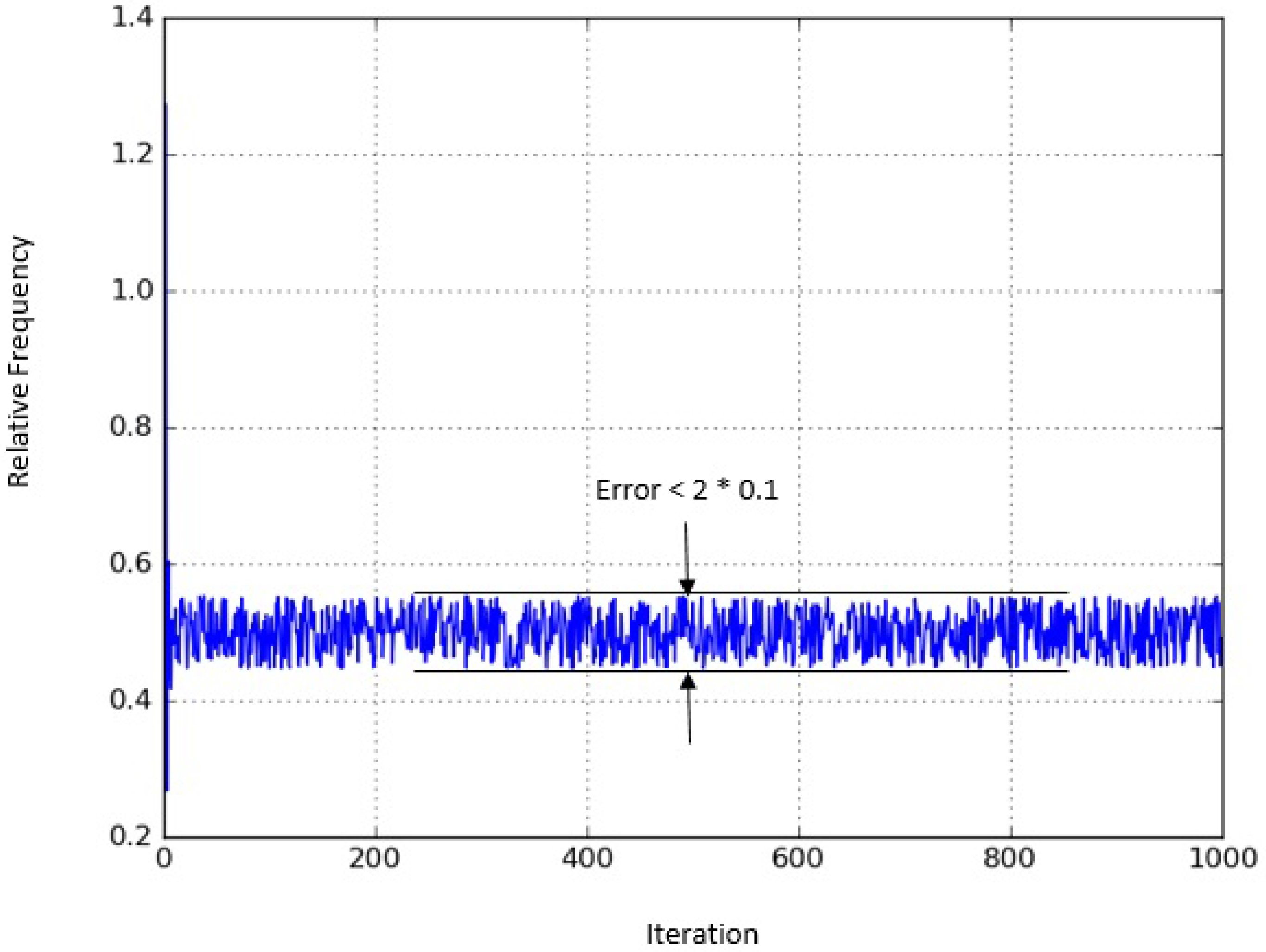
Now we demonstrate via numerical results that the obtained bounds indeed hold. Moreover, they are achievable after a small number of Markov chain steps, that is, with fast convergence. We simulated the example with the following parameters: $n=100$ states, $p_0=q_0=0.25$, and $ϵ=0.1$. The set A was a randomly chosen subset of 50 states. The transition probabilities were also chosen randomly, with the restriction that together with the other parameters they had to satisfy conditions (A), (B), (C).

Figure 1 shows the relative frequency of visiting A, as function of the number of Markov chain steps. It is well detectable that the chain converges quite slowly. Even after many iterations the deviation from the stationary probability $\pi \left(A\right)$ does not visibly tend to 0. On the other hand, it indeed stays within our error bound:

$$|{\pi }_t\left(A\right)-\pi \left(A\right)|\le \frac{ϵ}{p_0+q_0}=\frac{0.1}{0.25+0.25}=2\times 0.1$$

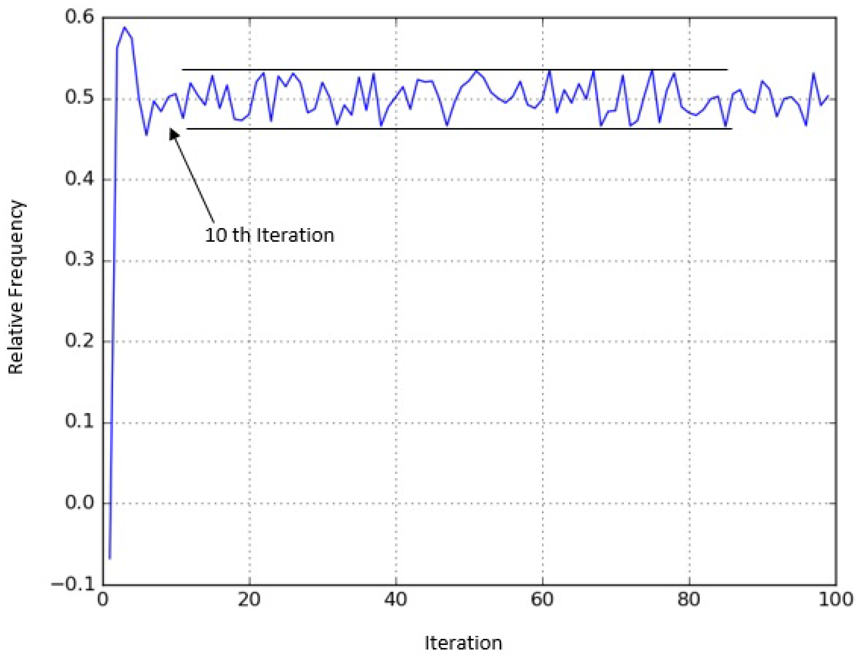
as promised. Having observed this, it is natural to ask, how soon can we reach this region, that is, how many steps are needed to satisfy the bound? This is shown in Figure 2. We can see that after only 10 iterations, the error bound is already satisfied. Note that this is very fast convergence, since the number of steps to get within the bound was as little as 10% of the number of states.

5. Conclusions

We have analyzed the convergence rate of quasi-lumpable Markov Chains. This represents the case when the large state space can be aggregated into a smaller number of clusters, in which the states behave approximately the same way. Our main contribution is a bound on the rate at which the aggregated state distribution approaches its limit in such chains. We have also demonstrated that in certain cases this can lead to a significantly accelerated convergence to an approximate estimation of the measure of subsets. The result can serve as a useful tool in the analysis of complex networks, when they have a clustering that approximately satisfies the conditions lumpability.