
Semi-Supervised Classification Based on Low Rank Representation


College of Computer and Information Science, Southwest University, Chongqing 400715, China
*
Author to whom correspondence should be addressed.
Algorithms 2016, 9(3), 48; https://doi.org/10.3390/a9030048
Submission received: 1 June 2016
/
Revised: 14 July 2016
/
Accepted: 20 July 2016
/
Published: 22 July 2016
Abstract
:Graph-based semi-supervised classification uses a graph to capture the relationship between samples and exploits label propagation techniques on the graph to predict the labels of unlabeled samples. However, it is difficult to construct a graph that faithfully describes the relationship between high-dimensional samples. Recently, low-rank representation has been introduced to construct a graph, which can preserve the global structure of high-dimensional samples and help to train accurate transductive classifiers. In this paper, we take advantage of low-rank representation for graph construction and propose an inductive semi-supervised classifier called Semi-Supervised Classification based on Low-Rank Representation (SSC-LRR). SSC-LRR first utilizes a linearized alternating direction method with adaptive penalty to compute the coefficient matrix of low-rank representation of samples. Then, the coefficient matrix is adopted to define a graph. Finally, SSC-LRR incorporates this graph into a graph-based semi-supervised linear classifier to classify unlabeled samples. Experiments are conducted on four widely used facial datasets to validate the effectiveness of the proposed SSC-LRR and the results demonstrate that SSC-LRR achieves higher accuracy than other related methods.
1. Introduction
In many machine learning tasks, one often lacks of sufficient labeled samples, which are usually difficult or expensive to accumulate. However, unlabeled samples are easy to obtain or collect. To get an accurate classifier, it is necessary to develop techniques that can leverage limited labeled samples and many unlabeled samples. Semi-supervised learning is one of the techniques that can take advantage of both the labeled and unlabeled samples, and it shows improved learning results compared with using scarce labeled data alone [1].
In this paper, we focus on graph based semi-supervised classification (GSSC). GSSC uses a graph to represent the data structure, where V is a set of vertices and each vertex represents a sample, is a set of edges connecting samples, and W is an adjacency matrix recording the weight of edges (or similarity) between samples. GSSC often exploits a graph-based regularization framework to classify unlabeled samples [1]. Zhu et al. [2] proposed an approach called Gaussian random fields and harmonic function (GFHF). GFHF predicts the labels of unlabeled samples by propagating labels of labeled samples on a k nearest neighborhood (kNN) graph. It is based on the consistency assumption that nearby points are likely to have similar outputs and points on the same structure (typically referred to as a cluster or a manifold) are likely to have the same label. Zhou et al. [3] introduced a local and global consistent (LGC) method to classify unlabeled samples on a kNN graph. Nevertheless, in essence, most graph-based semi-supervised classification algorithms are transductive; they cannot directly extend to new samples outside of the graph [1]. To perform inductive classification, Zhu et al. [4] suggested predicting the labels of unlabeled samples in the training set at first, and then labeling a new sample based on the labels of its nearest neighbors in the training set. That suggestion is only sensible when the number of unlabeled samples is sufficiently large and the predicted labels of unlabeled samples in the training set are correct.
Researchers have recognized that the graph determines the performance of GSSC [1,5,6]. However, how to construct a graph that correctly reflects the underlying distribution structure of samples is a public problem [1]. That is principally because the distance between samples becomes isometric as the dimensionality of samples increases [7]. Furthermore, many traditional similarity metrics are distorted by noisy or redundant features of high-dimensional data. For these reasons, researchers move forward to graph optimization based semi-supervised classification. Wang et al. [5] introduced a linear neighborhood propagation (LNP) method. LNP optimizes edge weights of a predefined kNN graph via minimizing the reconstruction error of a sample to its k nearest neighborhood samples by using an objective function similar to local linear embedding [8]. Zhao et al. [9] proposed a method called compact graph based semi-supervised learning (CGSSL). CGSSL infers labels of unlabeled samples by using an -graph, which is constructed by utilizing neighborhood samples of a sample and neighborhood samples of its reciprocal neighbors. Cheng et al. [10] proposed an -graph based transductive classifier by using sparse representation regularized with -norm, and the graph is constructed based on sparse representation coefficients. Fan et al. [11] proposed a sparse representation regularized least square classification (S-RLSC). To speed up the solution of sparse representation, Yu et al. [12] proposed a semi-supervised classification based on subspace sparse representation (SSC-SSR). SSC-SSR solves the -norm regularized sparse representation problem in several random subspaces, and trains a semi-supervised linear classifier on the -graph defined by the sparse representation coefficients in each subspace, and then combines these classifiers into an ensemble classifier. Sparse representation forces the coefficients to be sparse. Low rank representation was recently introduced to GSSC [13]. Yang et al. [13] constructed a graph by using the calculated low rank representation coefficients of both labelled and unlabeled samples as the graph weights, and incorporated that graph into GFHF for transductive classification. Low rank representation forces the coefficient matrix to be low rank and optimizes the matrix as a whole, whereas sparse representation often optimizes the coefficients per sample. It is recognized that low-rank is an appropriate approach for capturing the global structure of the data and the global mixture of subspace structure [14,15]. Peng et al. [16] proposed structure preserving low-rank representation technique by enforcing the local affinity property to be preserved without distorting the distant repulsion property and by utilizing the label information. Yang et al. [17] integrated the kernel trick with low rank representation, and introduced a kernel low-rank representation graph for GSSC. However, these approaches focus on transductive classification. Similar to LGC and GFHF, they cannot directly apply to samples outside of the graph.
In this paper, we introduce an inductive semi-supervised classifier based on low-rank representation (SSC-LRR). SSC-LRR first constructs a graph based on the low-rank representation coefficients. Next, it incorporates this graph into a graph-based semi-supervised linear classifier to classify unlabeled samples that are outside of the graph. Experimental results on four high-dimensional facial image datasets demonstrate that SSC-LRR performs better than other related GSSC methods. In addition, SSC-LRR is robust to noisy features and input parameters.
The remainder of this paper is organized as follows. In Section 2, we give the details of how to construct a graph by low rank constraints and introduce inductive semi-supervised classification based on a low rank. Section 3 provides the experimental results and analysis, followed with conclusions in Section 4.
2. Methodology
In this section, we present a semi-supervised classification based on low rank representation (SSC-LRR).
2.1. Low-Rank Representation for Graph Construction
Let be a set of samples, each column represents a sample. Each sample can be viewed as a linear combination of bases from a dictionary . Similar to work in [13,15], we set in this paper. Low rank representation represents each sample by a linear combination of the bases in as follows:
where is the coefficient matrix of low-rank representation. Each element in can be viewed as the contribution to the reconstruction of with as the dictionary. is often over complete. Therefore, Equation (1) cannot be solved in finite steps. To overcome this problem, we enforce to be low rank and solve the following optimization problem:
Obviously, is reconstructed by the low rank constrained matrix and the dictionary matrix . Equation (2) is coined as low rank representation (LRR) [15]. is added since Zhuang et al. In [18], it was observed that non-negative often leads to improved performance for data representation and graph construction. However, Equation (2) is NP-hard. Fortunately, Equation (2) can be relaxed to the following problem:
where is the nuclear norm of and it is the sum of singular values of [19]. Equation (3) can be solved by matrix completion methods [20]. Equation (3) can be further relaxed to take into account noisy features as follows:
where is called -norm [21] and is used to balance the effect of noise. The -norm encourages the columns of to be zero. To solve Equation (4), Lin et al. [22] suggested a Linearized Alternating Direction Method with Adaptive Penalty(LADMAP) technique to iteratively optimize and with each of them fixed as constant while optimizing the other. Next, each column of is normalized via , and then each negative entry of is set to zero. Low rank representation jointly finds the low-ranked coefficient matrix for all samples in . can be used to define a low rank representation based undirected graph, whose weighted adjacent matrix is .
2.2. Semi-Supervised Classification Based on Low Rank Representation
Suppose there are samples , where the first l samples are labeled and the left u samples are unlabeled. is the label vector of labeled samples and is the label of sample . To perform multi-class classification, we extend the label vector into a label matrix as:
For unlabeled sample , its corresponding label vector is a zero vector.
The general form of a linear classifier can be defined as:
where is the predictive matrix, is the label bias, is the predicted likelihood vector for with respect to C different labels.
Here, we consider a graph-regularized semi-supervised linear classifier as follows:
where the first term is the empirical loss on labeled samples, the second term is to take advantage of the global structure of samples, the last term controls the complexity of and to avoid over-fitting. The first term is defined as follows:
where tr() is the matrix trace operator, is an diagonal matrix with if is labeled, =0 otherwise. is an N-dimensional vector with all elements are set to 1. The second term of Equation (7) can be computed as:
where is the weight of edge between and , and is the low rank representation coefficient matrix obtained from Equation (4). is a diagonal matrix with , is the graph Laplacian matrix [23]. The last term of Equation (7) is used to control the complexity of , it is computed as follows:
Equation (11) can be solved by taking partial derivative of with respect to and as below:
Let and , we can obtain:
where is:
Given and are already known, , is mainly determined by . Here, is the weighted adjacent matrix of a graph constructed by low rank representation coefficient matrix (see Equation (4)). In contrast to the transductive classifier, our proposed SSC-LRR directly uses and to predict the likelihood of with respect to C classes. The predicted label of is:
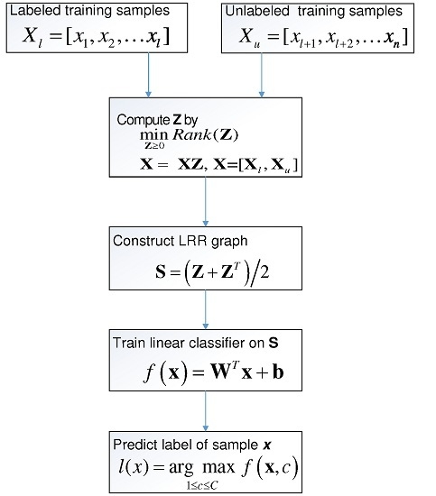
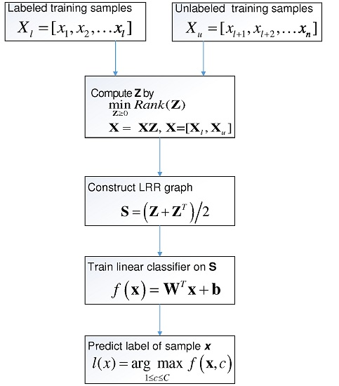
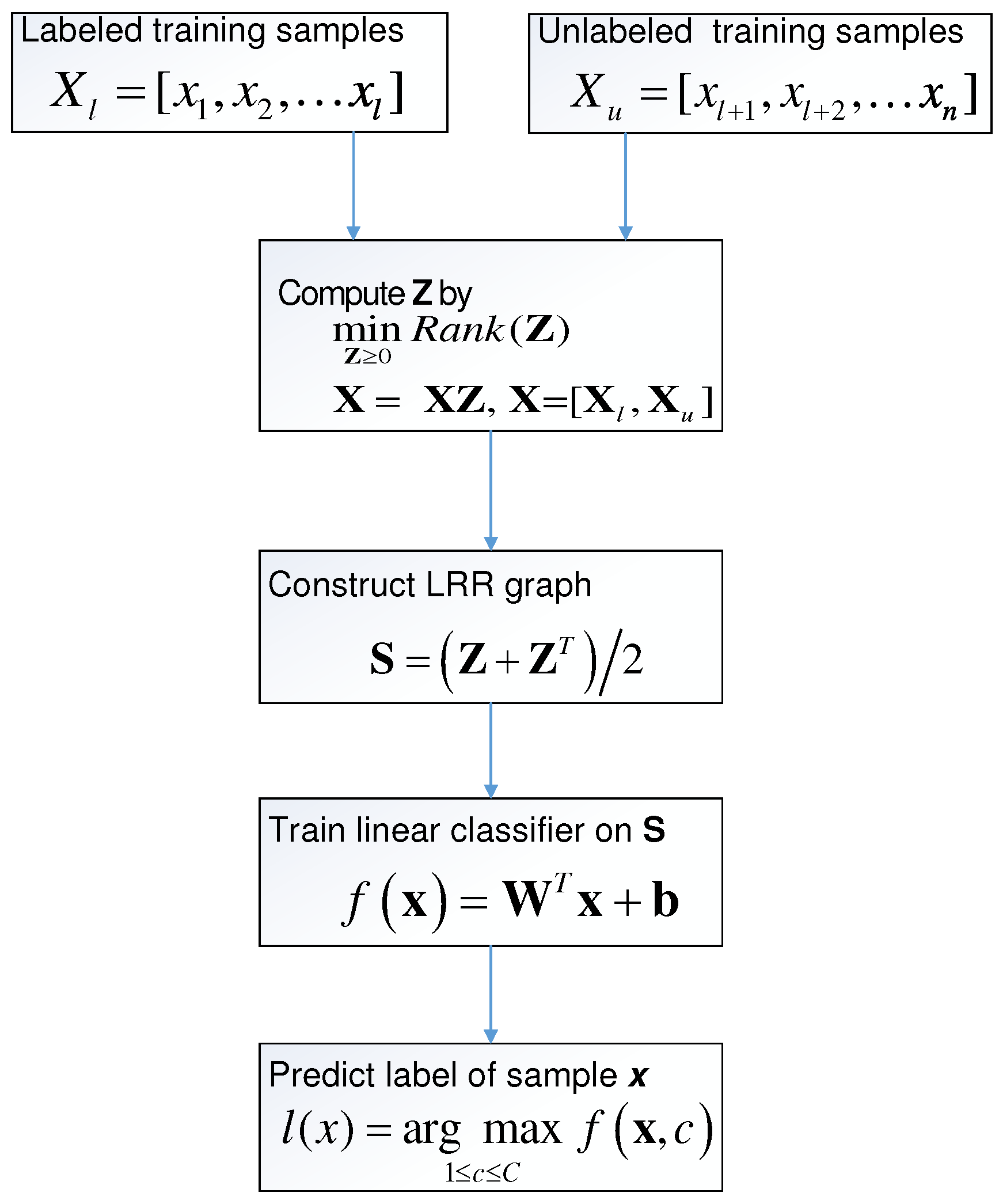
where indicates the c-th entry of , and is the predicted label of . Figure 1 briefly lists the process of SSC-LRR algorithm.
3. Experiments
3.1. Experiments Setup
In this section, we conduct experiments on four facial datasets AR [24], ORL [25], PIE [26] and YaleB [27] to validate the effectiveness of our proposed SSC-LRR with several related and representative graph-based semi-supervised classification methods: GFHF [2], LGC [3], LNP [5], CGSSL [9], LRR-GFHF [18], S-RLSC [11] and LRR-MR. LGC and GFHF use kNN graph, CGSSL and LNP employ graph , S-RLSC uses -graph. LRR-GFHF constructs a graph by utilizing coefficient matrix in Equation (4), and then applies GFHF on this graph to classify unlabeled samples. LRR-MR uses the same graph as LRR-GFHF and SSC-LRR, but it employs a representative semi-supervised nonlinear classifier- manifold regularization (MR) [28] on the graph to predict the label of unlabeled samples. GFHF, LGC, CGSSL and LRR-GFHF are transductive classifiers that can not directly classify out-of-sample, which is currently not in the graph. We extend them for out-of-sample situations by setting the label of a new sample as the label of its nearest training sample, and the labels of unlabeled training samples are predicted by the respective transductive classifier in advance. Notably, S-RLSC, LRR-MR and SSC-LRR directly use all the labeled and unlabeled samples to predict the label of a new sample, without predicting the labels of unlabeled training samples in advance.
AR contains 2600 images of 100 persons. These images are transformed into grayscale and cropped into 42 × 30 pixels. Thus, each image can be viewed as a point in the 1260-dimensional space. For each person, we choose 13 images as training set, and set the rest ones as testing set. YaleB contains 2414 images of 38 people, and each image is cropped into 32 × 32 pixels, and then transformed into grayscale images. For each person, we choose 20 images per person as training set, the remaining samples as testing set. ORL contains 400 face images of 40 people, and each image is cropped into 32 × 32 pixels and transformed into a grayscale image. For each person, we select six images per person as training set, and remaining four images as testing set. PIE includes 41,368 face images of 68 individuals. In the experiment, we select the subset Pose27 (including 3329 images) for experiments and crop these images to 64 × 64 pixels. For each person, we select 20 pictures of each person as training set and the rest images as testing set.
For presentation, we introduce several symbols: N-the number of training samples, -the number of testing samples, D-the dimensionality of samples, C-the number of classes, -the number of images per person in the training set, m-the number of labeled images per person in the training set, k-neighborhood size. In the experiments, unless extra specified, λ is set to 0.01, α is set to 0.05, β is set to 0.05, k is set to 5. To reduce random effect, all the experimental results are the average of 20 independent runs. In each run, we randomly select a fixed number of samples from the training set as labeled samples, and the remaining samples of training set are used as unlabeled samples.
3.2. Accuracy with Respect to Different Number of Labeled Samples
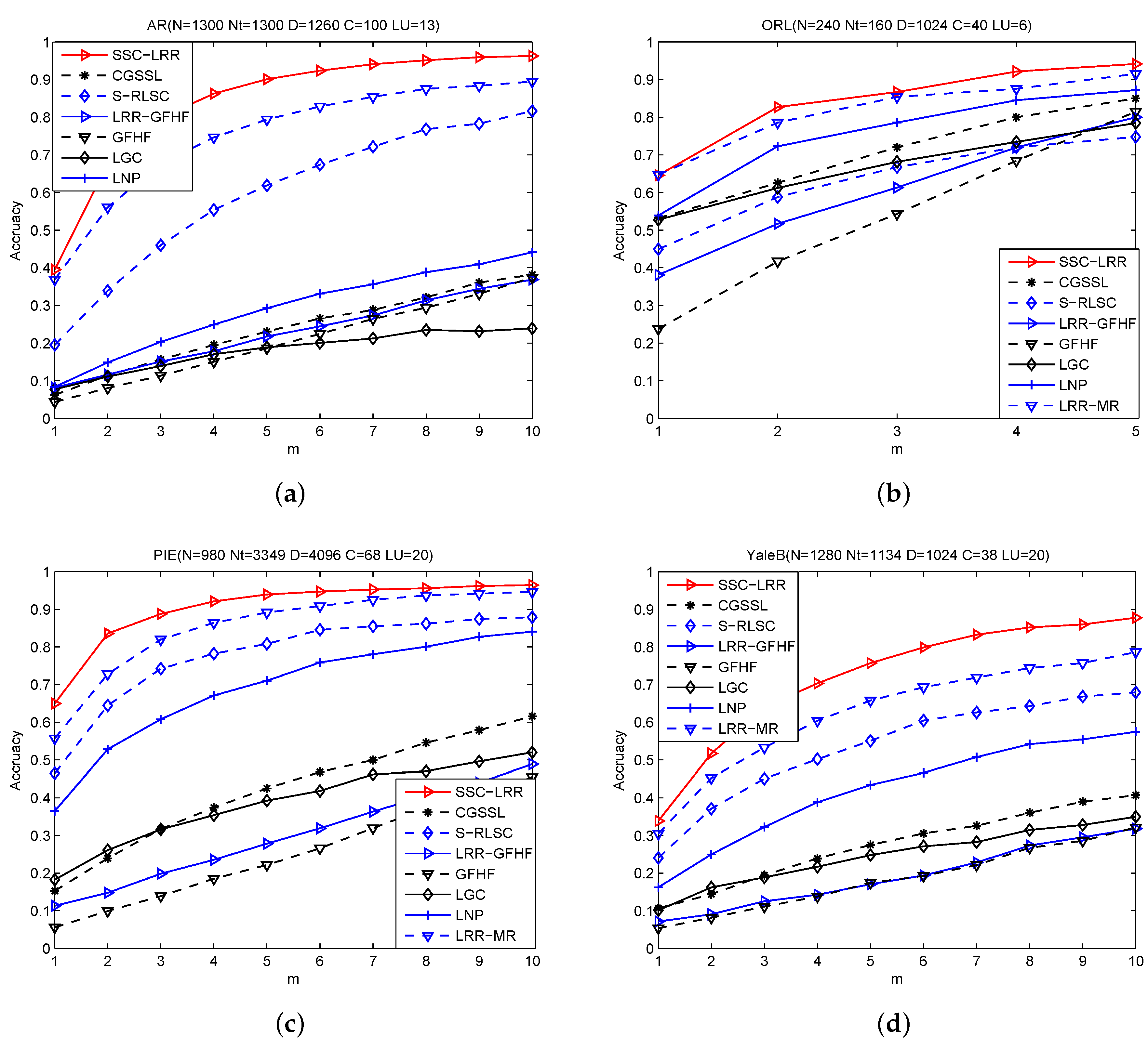
In order to study the influence of the number of labeled samples on the accuracy of semi-supervised classification, we conduct experiments on AR, PIE, and YaleB by varying m from 1 to 10, on ORL by varying m from 1 to 5. The recorded results are plotted in Figure 2.
From Figure 2, we can observe that the accuracy of all methods increases with the number of labeled samples m rising and SSC-LRR always achieves better performance than other comparing methods. GFHF and LGC use a single kNN graph, while LGC outperforms GFHF. That is because LGC classifies samples based on the consistency assumption. This fact indicates that the consistency assumption can improve the performance of the algorithm in a small range. GFHF and LRR-GFHF use the same classifier, while the accuracy of GFHF is much lower than that of LRR-GFHF. This fact shows that LRR-based graph can better reflect the relationship between samples than kNN graph. The accuracy of LGC is lower than that of CGSSL and LNP, which utilize an optimized -graph by different techniques. The cause is that LGC uses a single kNN graph, which can be easily destroyed by noisy featured. In contrast, -graph is more effective than kNN graph in capturing the similarity relationship between samples. These observations also corroborate that graph determines the performance of GSSC methods.
S-RLSC uses a single graph, and achieves better performance than CGSSL and LNP on AR, PIE and YaleB. This fact coincides with previous study that -graph is generally more effective than graph based semi-supervised classification methods [12]. However, the accuracy of S-RLSC is lower than that of LNP on ORL, since ORL has a relative small number of training samples and -graph asks for a large number of basic samples to optimize the sparse representation coefficients.
Compared with GFHF, LGC, LNP and CGSSL, both the -graph and LRR based graph demonstrate better ability to capture the relationship between high-dimensional samples. We want to remark that SSC-LRR achieves higher accuracy than S-RLSC, although both of them are inductive classifiers. The reason is that LRR graph has better capacity in exploiting the global data structure of samples than graph. The performance margin between S-RLSC and SSC-LRR on AR is more obvious than that on other facial databases, since there are more noises in the images of AR than that of other datasets. This fact shows SSC-LRR is more robust to noise than and graphs. LRR-GFHF, LRR-MR and SSC-LRR employ LRR to construct a graph for semi-supervised classification, SSC-LRR and LRR-MR show improved accuracy than LRR-GFHF. This is principally because LRR-GFHF is extended to an inductive classifier by transferring the labels of labeled samples and pseudo labels of unlabeled samples to a new sample , but the pseudo labels of unlabeled samples in the training set are not correctly predicted. In contrast, SSC-LRR does not predict the labels of unlabeled samples in the training set, it directly exploits and in Equation (6) to predict the label of . LRR-MR is a non-linear inductive classifier, it often gets higher accuracy than other comparing methods, except SSC-LRR, although these adopted image datasets are not explicitly linear classifiable. This comparison shows that both linear classifiers and non-linear classifiers can achieve good performance by exploiting a LRR-based graph. These results support our motivation to use LRR for inductive semi-supervised classification.
3.3. Sensitivity Analysis on Input Parameters
To study the influence of the balance parameter λ (see Equation (4)) of LRR for SSC-LRR, we conduct additional experiments on AR, ORL, PIE, and YaleB by setting λ to 100, 10, 1, 0.1, and 0.01, respectively. The value of m on AR, ORL, PIE, and YaleB are fixed as 10, 5, 10, 10, respectively. The recorded results are plotted in Figure 3.
From Figure 3, we can observe that the value of λ has no obvious influence on the classification accuracy on each dataset. The performance of SSC-LRR almost remains the same within a relative large range of λ. Therefore, SSC-LRR is robust to input parameter λ, which balances the effect of noise and low rankness.
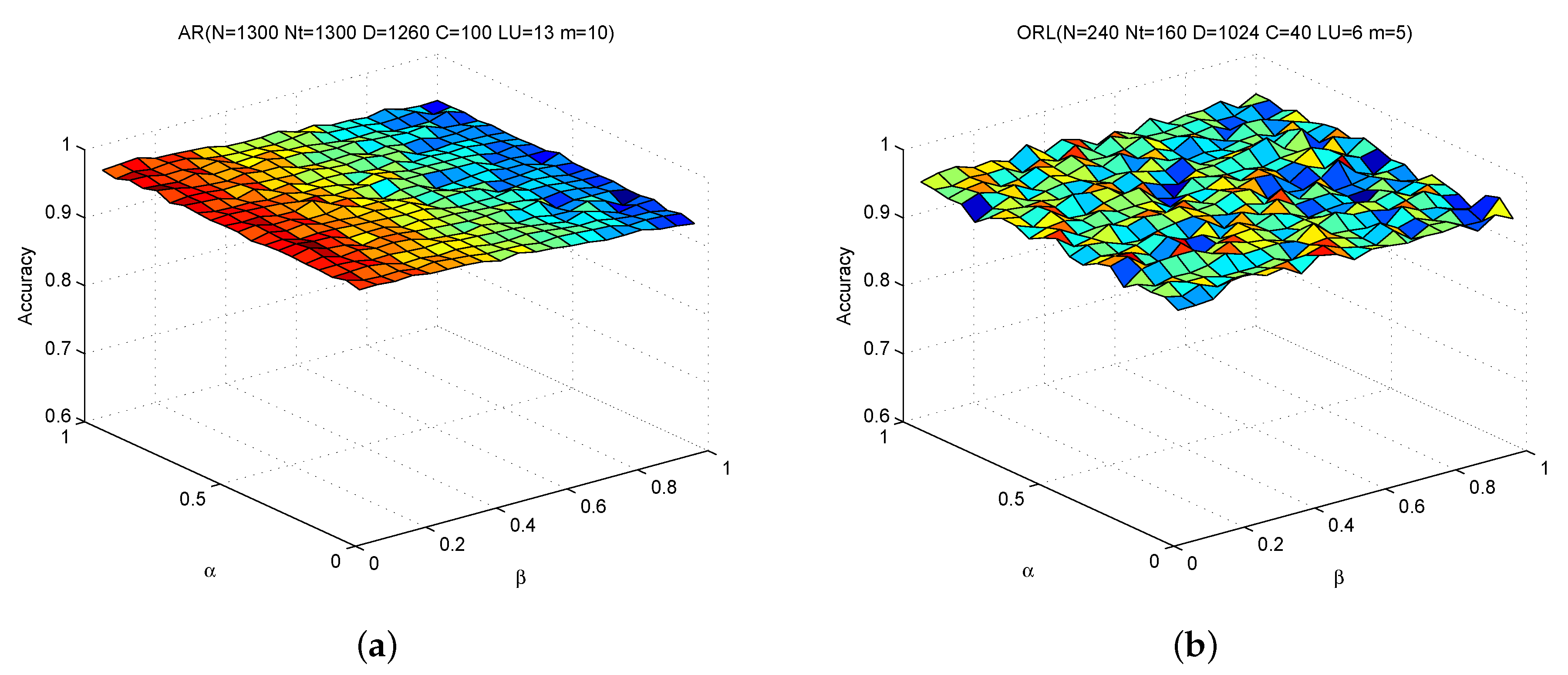
In addition, we also investigate the sensitivity of SSC-LRR with respect to α and β (see Equation (7)). We perform additional experiments on ORL and AR with both α and β rising 0.05 to 1 with stepsize 0.05. The value of m on AR and ORL are fixed as 10 and 5, respectively. The recorded results for each combination of α and β are revealed in Figure 4. From Figure 4, we can also observe that SSC-LRR achieves rather stable performance within a relative large range of α and β.
From these results, we can conclude SSC-LRR is robust to noise and can work well under a wide range of input values of parameters.
4. Conclusions
In this paper, we investigate how to boost the performance of graph-based semi-supervised classification by constructing a well structured graph. We employ low rankness representation to construct a weighted adjacent matrix between samples and incorporate this graph into a semi-supervised inductive classifier, and thus introduce a method called Semi-Supervised Classification based on Low-Rank Representation (SSC-LRR). Experimental results on four high-dimensional face datasets show that SSC-LRR not only has higher accuracy than other related methods, but is also robust to the input parameter. We are planning to study more effective and efficient techniques to construct a graph and to further enhance the performance of graph based semi-supervised classification.
Acknowledgments
This work is supported by Natural Science Foundation of China (61402378), Natural Science Foundation of CQ CSTC (cstc2014jcyjA40031 and cstc2016jcyjA0351), Fundamental Research Funds for the Central Universities of China (2362015XK07 and XDJK2016B009).
Author Contributions
Xuan Hou and Guangjun Yao performed experiments and drafted the manuscript; Jun Wang proposed the idea and conceived the whole process and revised the manuscript; All the authors read and approved the final manuscript.
Conflicts of Interest
The authors declare no conflict of interest.
References
- Zhu, X. Semi-Supervised Learning Literature Survey; Technical Report 1530; University of Wisconsin-Madison: Madison, WI, USA, 2008. [Google Scholar]
- Zhu, X.; Ghahramani, Z.; Lafferty, J. Semi-supervised learning using gaussian fields and harmonic functions. In Proceedings of the International Conference on Machine Learning, Washington, DC, USA, 21–24 August 2003; pp. 912–919.
- Zhou, D.; Bousquet, O.; Lal, T.; Weston, J.; Scholkopf, B. Learning with local and global consistency. Adv. Neural Inf. Process. Syst. 2004, 16, 321–328. [Google Scholar]
- Zhu, X.; Lafferty, O.J.; Ghahramani, Z. Semi-Supervised Learning: From Gaussian Fields to Gaussian Processes; Technical Report CMU-CS-03-175; Carnegie Mellon University: Pittsburgh, PA, USA, 2003. [Google Scholar]
- Wang, J.; Wang, F.; Zhang, C.; Shen, H.; Quan, L. Linear neighborhood propagation and its applications. IEEE Trans. Pattern Anal. Mach. Intell. 2009, 31, 1600–1615. [Google Scholar] [CrossRef] [PubMed]
- Liu, W.; Chang, S. Robust multi-class transductive learning with graphs. In Proceedings of the IEEE Conference on Computer Vision and Pattern Recognition, Miami, FL, USA, 20–25 June 2009; pp. 381–388.
- Parson, L.; Haque, E.; Liu, H. Subspace clustering for high dimensional data: A review. ACM SIGKDD Explor. Newsl. 2004, 6, 90–105. [Google Scholar] [CrossRef]
- Roweis, S.T.; Saul, L.K. Nonlinear dimensionality reduction by locally linear embedding. Science 2000, 290, 2323–2326. [Google Scholar] [CrossRef] [PubMed]
- Zhao, M.; Chow, T.W.; Zhang, Z.; Li, B. Automatic image annotation via compact graph based semi-supervised learning. Knowl.-Based Syst. 2015, 76, 148–165. [Google Scholar] [CrossRef]
- Cheng, B.; Yang, J.; Yan, S. Learning With l1 Graph for Image Analysis. IEEE Trans. Image Process. 2010, 19, 858–866. [Google Scholar] [CrossRef] [PubMed]
- Fan, M.; Gu, N.; Qiao, H.; Zhang, B. Sparse regularization for semi-supervised classification. Pattern Recognit. 2011, 44, 1777–1784. [Google Scholar] [CrossRef]
- Yu, G.; Zhang, G.; Zhang, Z.; Yu, Z.; Deng, L. Semi-supervised classification based on subspace sparse representation. Knowl. Inf. Syst. 2015, 43, 81–101. [Google Scholar] [CrossRef]
- Yang, S.; Wang, X.; Wang, M.; Han, Y.; Jiao, L. Semi-supervised low-rank representation graph for pattern recognition. IET Image Process. 2013, 7, 131–136. [Google Scholar] [CrossRef]
- Liu, G.; Lin, Z.; Yan, S.; Sun, J.; Ma, Y. Robust recovery of subspace structures by low-rank representation. IEEE Trans. Pattern Anal. Mach. Intell. 2013, 35, 171–184. [Google Scholar] [CrossRef] [PubMed]
- Liu, G.; Lin, Z.; Yu, Y. Robust subspace segmentation by low-rank representation. In Proceedings of the 27th International Conference on Machine Learning, Haifa, Israe, 21–24 June 2010; pp. 663–670.
- Peng, Y.; Long, X.; Lu, B. Graph based semi-supervised learning via structure preserving low-rank representation. Neural Process. Lett. 2015, 41, 389–406. [Google Scholar] [CrossRef]
- Yang, S.; Feng, Z.; Ren, Y.; Liu, H.; Jiao, L. Semi-supervised classification via kernel low-rank representation graph. Knowl. Based Syst. 2014, 69, 150–158. [Google Scholar] [CrossRef]
- Zhuang, L.; Gao, H.; Lin, Z.; Ma, Y.; Zhang, X.; Yu, N. Non-negative low rank and sparse graph for semi-supervised learning. In Proceedings of the IEEE Conference on Computer Vision and Pattern Recognition, Providence, RI, USA, 16–21 June 2012; pp. 2328–2335.
- Cai, J.F.; Candès, E.J.; Shen, Z. A singular value thresholding algorithm for matrix completion. SIAM J. Optim. 2010, 20, 1956–1982. [Google Scholar] [CrossRef]
- Candès, E.; Li, X.; Ma, Y.; Wright, J. Robust principal component analysis. J. ACM 2011, 58, 11. [Google Scholar] [CrossRef]
- Liu, J.; Ji, S.; Ye, J. Multi-task feature learning via efficient l2,1-norm minimization. In Proceedings of the International Conference on Uncertainty in Artificial Intelligence, Montreal, QC, Canada, 18–21 June 2009; pp. 339–348.
- Lin, Z.; Liu, R.; Su, Z. Linearized alternating direction method with adaptive penalty for low-rank representation. In Proceedings of the Neural Information Processing Systems, Granada, Spain, 12–17 December 2011; pp. 612–620.
- Chung, F.R. Spectral Graph Theory; American Mathematical Society: Providence, RI, USA, 1997; Volume 92. [Google Scholar]
- Martinez, A.; Benavente, R. The AR-Face Database; Technical Report 24; Computer Vision Center: Barcelona, Spain, 1998. [Google Scholar]
- Samaria, F.; Harter, A. Parameterisation of a stochastic model for human face identification. In Proceedings of the the Second IEEE Workshop on Applications of Computer Vision, Sarasota, FL, USA, 5–7 December 1994; pp. 138–142.
- Sim, T.; Baker, S.; Bsat, M. The CMU Pose, Illumination, and Expression Database. IEEE Trans. Pattern Anal. Mach. Intell. 2003, 25, 1615–1618. [Google Scholar]
- Georghiades, A.; Belhumeur, P.; Kriegman, D. From few to many: Illumination cone models for face recognition under variable lighting and pose. IEEE Trans. Pattern Anal. Mach. Intell. 2001, 23, 643–660. [Google Scholar] [CrossRef]
- Belkin, M.; Niyogi, P.; Sindhwani, V. Manifold regularization: A geometric framework for learning from labeled and unlabeled examples. J. Mach. Learn. Res. 2006, 7, 2399–2434. [Google Scholar]
Figure 1.
Flowchart of Semi-Supervised Classification based on Low-Rank Representation (SSC-LRR) algorithm.
Figure 1.
Flowchart of Semi-Supervised Classification based on Low-Rank Representation (SSC-LRR) algorithm.

Figure 2.
Accuracy versus m (number of labeled images per person).

Figure 3.
Accuracy versus λ.
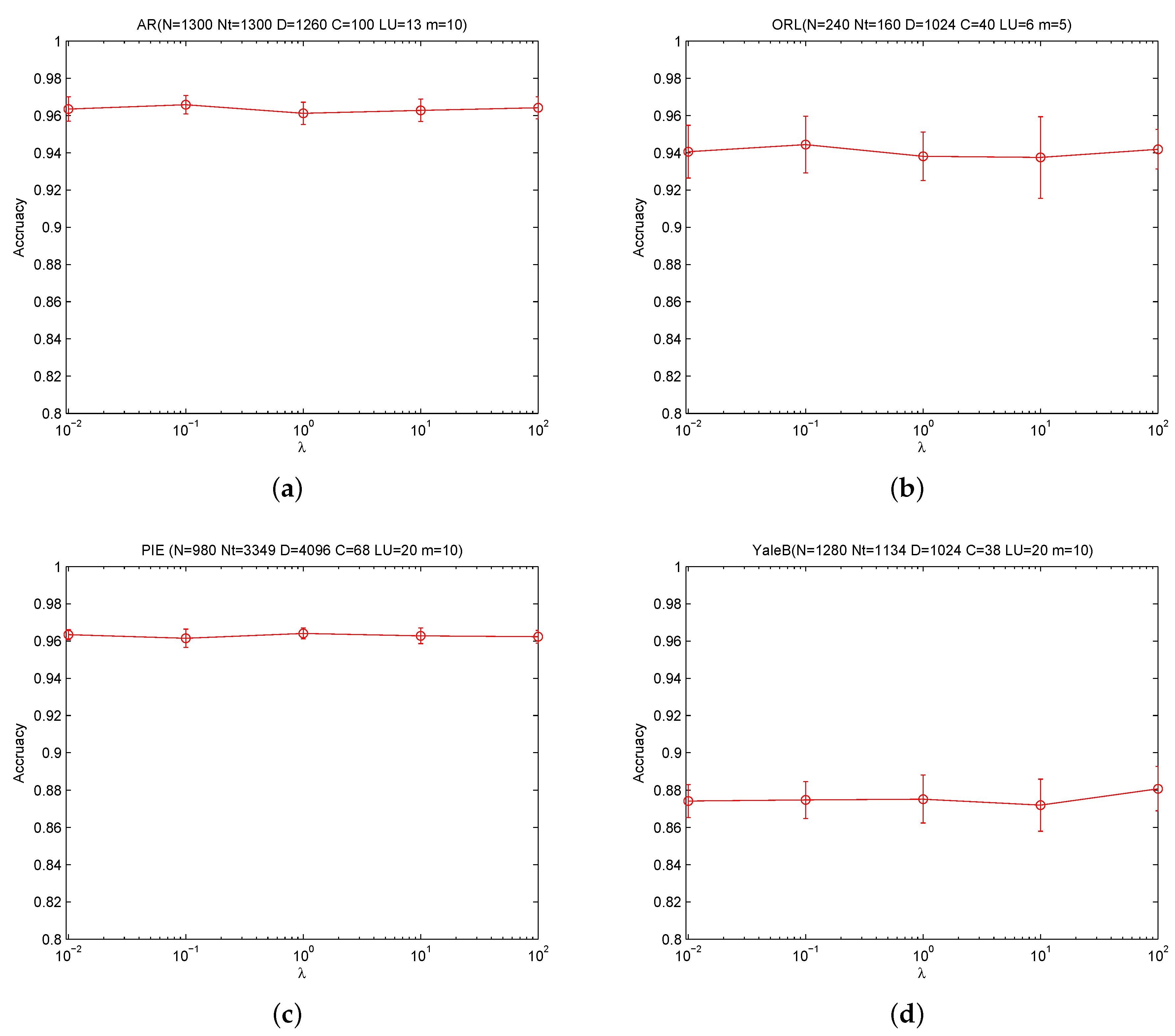
Figure 4.
Accuracy versus α and β.

© 2016 by the authors; licensee MDPI, Basel, Switzerland. This article is an open access article distributed under the terms and conditions of the Creative Commons Attribution (CC-BY) license (http://creativecommons.org/licenses/by/4.0/).
Share and Cite
MDPI and ACS Style
Hou, X.; Yao, G.; Wang, J. Semi-Supervised Classification Based on Low Rank Representation. Algorithms 2016, 9, 48. https://doi.org/10.3390/a9030048
AMA Style
Hou X, Yao G, Wang J. Semi-Supervised Classification Based on Low Rank Representation. Algorithms. 2016; 9(3):48. https://doi.org/10.3390/a9030048
Chicago/Turabian StyleHou, Xuan, Guangjun Yao, and Jun Wang. 2016. "Semi-Supervised Classification Based on Low Rank Representation" Algorithms 9, no. 3: 48. https://doi.org/10.3390/a9030048
Note that from the first issue of 2016, this journal uses article numbers instead of page numbers. See further details here.