Joint Antenna Selection and Beamforming Algorithms for Physical Layer Multicasting with Massive Antennas

Abstract

We investigate the problem of minimizing the total power consumption under the constraint of the signal-to-noise ratio (SNR) requirement for the physical layer multicasting system with large-scale antenna arrays. In contrast with existing work, we explicitly consider both the transmit power and the circuit power scaling with the number of antennas. The joint antenna selection and beamforming technique is proposed to minimize the total power consumption. The problem is a challenging one, which aims to minimize the linear combination of ${\ell }_0$-norm and ${\ell }_2$-norm. To our best knowledge, this minimization problem has not yet been well solved. A random decremental antenna selection algorithm is designed, which is further modified by an approximation of the minimal transmit power based on the asymptotic orthogonality of the channels. Then, a more efficient decremental antenna selection algorithm is proposed based on minimizing the ${\ell }_0$ norm. Performance results show that the ${\ell }_0$ norm minimization algorithm greatly outperforms the random selection algorithm in terms of the total power consumption and the average run time.

1. Introduction

Physical layer multicasting with a base station (BS) transmitting a common information to multiple terminals simultaneously has attracted intensive attentions recently. This system can support various applications such as the delivery of headline news, service information, and live broadcast, etc. Sidiropoulos et al. [1] studied the transmit power minimization problem constrained by the signal-to-noise ratios (SNRs) of a group of receivers. In addition to proving the NP hardness of the problem, they optimized the beamforming vector using the semidefinite relaxation (SDR) and randomization techniques. The problem for multiple cochannel groups was investigated in [2]. Since the number of antennas (N) is usually more than the number of available radio frequency (RF) chains (K) at the BS, the joint antenna selection and beamforming for a single group and multiple cochannel groups was studied in [3,4], respectively. Through jointly selecting K antennas from the total N antennas and optimizing the beamforming vector, the transmit power is minimized while meeting the quality of service (QoS) requirement of each receiver. Compared with the routine SDR approach, Tran et al. have solved the transmit power minimization problem using a successive convex approximation (SCA) approach with a massively reduced computational complexity [5]. Because of the low computational complexity, the SCA approach is suitable for the physical layer multicasting system with large-scale antenna arrays.

The multiple-input multiple-output (MIMO) system with large-scale antenna arrays was proposed in [6], and has been intensively studied for a higher spectral efficiency, reduced signal processing complexity, and improved energy efficiency compared with the traditional MIMO [7,8]. It is shown that the required transmit power to support a target rate is inversely proportional to the number of antennas in the massive MIMO system [9]. The optimal configurations of the RF chains was studied in [10] to maximize the transmit rate under the total power consumption constraint with or without the channel state information (CSI).

In the existing literature, the transmit power has been minimized, while the circuit power is neglected. However, the circuit power actually scales with the number of antennas and it should be considered for MIMO systems, especially the massive MIMO. In contrast to previous work, this paper aims to minimize the total power consumption under the SNR constraint of each receiver through jointly determining the antenna subset and the beamforming vector. Since the circuit power depends directly on the number of active RF chains in the antenna selection, we explicitly consider the circuit power in the total power consumption model. The main contributions of this paper are detailed as follows:

• We formulate the total power consumption minimization problem by joint antenna selection and beamforming for physical layer multicasting with massive antennas.
• Due to the higher complexity of the exhaustive search for the optimal solution, we propose three decremental antenna selection algorithms for the sub-optimal solution with low complexity.
• On the basis of the SCA approach, we propose an algorithm to randomly select the antenna in a decremental manner, and modify the algorithm using the asymptotic orthogonality of the channels to improve the computational efficiency.
• Instead of random selection, a more effective algorithm is further proposed based on the ${\ell }_0$ norm minimization.
• Simulation results are provided to compare the performance of our proposed algorithms in terms of the total power consumption and the average run time.

The paper is organized as follows. Section 2 formulates the total power minimization problem. Three decremental antenna selction algorithms are proposed in Section 3. Simulation results are provided in Section 4 and conclusions are drawn in Section 5.

Notations: Throughout this paper, scalers and vectors are denoted by lowercase letters and boldface lowercase letters, respectively. For any vector, the superscript ${\left(·\right)}^H$ denotes the Hermitian transpose. The notations $\left|·\right|$ and ${∥·∥}_2$ denote the absolute value and 2-norm, respectively. We use $\mathcal{CN}\left(m,{\sigma }^2\right)$ to denote the circular symmetric complex Gaussian distribution with mean m and covariance ${\sigma }^2$.

2. Problem Formulation

We consider the physical-layer multicasting system, where a single BS equipped with N antennas and N RF chains broadcasts a common message to M single antenna receivers. The received signal at the receiver i is given as

$$y_i=\sqrt{{\beta }_i}{\mathit{h}}_i^H\mathit{w}s+n_i$$

(1)

where $s\sim \mathcal{CN}(0,1)$ is the common signal transmitted to M receivers. $\sqrt{{\beta }_i}$ and the $N\times 1$ vector ${\mathit{h}}_i\sim \mathcal{CN}(0,{\mathbf{I}}_N)$ represent the large-scale and small-scale fading of the i-th receiver’s channel, respectively. $\mathit{w}\in {\mathbb{C}}^N$ is the beamforming vector and $n_i\sim \mathcal{CN}(0,{\sigma }_i^2)$ is the additive white Gaussian noise at the receiver i. The received SNR of the i-th receiver is

$${\gamma }_i={\beta }_i{\left|{\mathit{w}}^H{\mathit{h}}_i\right|}^2/{\sigma }_i^2$$

(2)

Considering the circuit power of the RF chains, the total power minimization problem can be formulated as:

$$\begin{array}{cc}\hfill {\mathcal{P}}_1:\underset{\mathbf{w}\in {\mathbb{C}}^N}{min}& \frac{{\parallel \mathbf{w}\parallel }_2^2}{\eta }+P_{\mathrm{cir}}{∥\mathit{w}∥}_0\hfill \\ \hfill \mathrm{s}.\mathrm{t}.& |{\mathit{w}}^H{\mathbf{h}}_i{|}^2\ge {\overline{\gamma }}_i,i=1,\dots ,M\hfill \end{array}$$

(3)

where ${\overline{\gamma }}_i={\tilde{\gamma }}_i{\sigma }_i^2/{\beta }_i$ with ${\tilde{\gamma }}_i$ denoting the SNR threshold of the i-th receiver. In the objective function, the first term represents the transmit power with η denoting the power amplifier efficiency, and the second term represents the circuit power consumption with $P_{\mathrm{cir}}$ denoting the circuit power cost per RF chain. The ${\ell }_0$-norm ${∥\mathbf{w}∥}_0:=\left|\left\{n:{\mathbf{w}}_n\ne 0\right\}\right|$ represents the number of nonzero entries of the beamforming vector $\mathbf{w}$, where ${\mathbf{w}}_n$ represents the n-th element of $\mathbf{w}$. We can select the antenna subset corresponding to the nonzero entries of the beamforming vector and the unnecessary RF chains are switched off to reduce the circuit power consumption. The circuit power consumption is proportional to the number of active RF chains ${∥\mathbf{w}∥}_0$. The total consumed power comprises of both the transmit power and the circuit power of the RF chains.

3. Decremental Antenna Selction Algorithms

Since the ${\ell }_0$-norm is non-convex and it has no accurate approximations, it is difficult to solve the optimization problem ${\mathcal{P}}_1$. To our best knowledge, there exists no approach to minimize the linear combination of ${\ell }_0$-norm and ${\ell }_2$-norm. The optimal solution can be found by exhaustive searching $2^N$ antenna subsets, i.e., solving the following NP-hard problem with $2^N$ times,

$$\begin{array}{cc}\hfill {\mathcal{P}}_2:\underset{\mathbf{w}\in {\mathbb{C}}^N}{min}& {\parallel \mathbf{w}\parallel }_2^2\hfill \\ \hfill \mathrm{s}.\mathrm{t}.& |{\mathbf{w}}^H{\mathbf{h}}_i{|}^2\ge {\overline{\gamma }}_i,i=1,\dots ,M\hfill \end{array}$$

(4)

The complexity is enormous when the BS is equipped with large-scale antenna arrays. An iterative SCA algorithm has been proposed by Tran et al. to solve the problem ${\mathcal{P}}_2$ effectively [5]. In this sections, we try to find the near-optimal solution by jointly optimizing the antenna subset and its beamforming vector.

Theorem 1. 

Let Υ and Φ denote two antenna subsets with the relationship ${\rm Y}\subset \Phi$. ${\mathbf{w}}_{{\rm Y}}^{opt}$ and ${\mathbf{w}}_{\Phi }^{opt}$ are the optimal beamforming vectors regarding to Υ and Φ, respectively. The minimal transmission power consumed by the antenna subset Υ is no less than that of Φ, i.e., ${∥{\mathbf{w}}_{{\rm Y}}^{opt}∥}_2^2\ge {∥{\mathbf{w}}_{\Phi }^{opt}∥}_2^2$.

Proof. 

Let ${\mathbf{w}}_{\Phi }=({\mathbf{w}}_{{\rm Y}}^{\mathrm{opt}};\mathbf{0})$, then the elements of beamforming vector corresponding to the antenna subset $\Delta =\Phi -{\rm Y}$ equal zero. It is obvious that ${∥{\mathbf{w}}_{{\rm Y}}^{\mathrm{opt}}∥}_2^2={∥{\mathbf{w}}_{\Phi }∥}_2^2\ge {∥{\mathbf{w}}_{\Phi }^{\mathrm{opt}}∥}_2^2$. ☐

As can be seen from Theorem 1, with the shrinking of the antenna subset, the minimal transmit power consumption gets larger, while the circuit power consumption gets smaller. Therefore, we can determine a tradeoff between the circuit power and the transmit power through designing the decremental antenna selection algorithms. The initial antenna subset is defined as $S_{\left(0\right)}$ with all the antennas selected. In each iteration, a new antenna subset is obtained from the previous subset according to different methods. The iteration of antenna selection continues when the total power consumption of the new antenna subset is less than the previous antenna subset. So, in each step of the antenna selection, we can make sure that the obtained new subset is superior to the previous subset and it is thus updated. Otherwise, when the total power consumption of the current iteration is no less than the previous subset, the antenna selection process is terminated. In this process, the total power consumption decreases step by step. Inspired by this fact, we proposed three decremental antenna selection algorithms based on the SCA approach.

3.1. Random Decremental Selection (RDS) Algorithm

We first propose a random decremental selection (RDS) algorithm. In the r-th step, k antennas are randomly selected from the antenna subset $S_{(r-1)}$ and removed, the new subset is $S_{\left(r\right)}$. Then, we calculate the minimal transmit power consumption of $S_{\left(r\right)}$ using the SCA approach as it leads to an efficient solution with lower transmit power consumption compared with the routine SDR approach [1]. The total consumed power of $S_{\left(r\right)}$ can be obtained by summing the circuit power and the minimal transmit power calculated by the SCA approach [5]. If the antenna subset $S_{\left(r\right)}$ consumes less power than $S_{(r-1)}$, the algorithm goes into the next step, otherwise, the algorithm should be terminated with $S_{(r-1)}$ being the selected best antenna subset. Since k antennas are randomly selected and removed from the previous subset in each iteration, the tradeoff between the system performance and the algorithm efficiency can be balanced by judiciously adjusting the parameter k.

3.2. Modified Random Decremental Selection (MRDS)

To improve the efficiency of the RDS algorithm, we further propose the modified random decremental selection (MRDS) algorithm through introducing an effective and accurate approximation of the minimal transmit power consumption based on the asymptotic orthogonality of the channels [11]. The asymptotic orthogonality reduces the complexity of signal processing. To maximize the minimum SINR of all the users constrained by the transmit power, Xiang et al. proved that the asymptotically optimal beamformer when $N\to \infty$ is a linear combination of the channels between the BS and its served users [12].

Theorem 2. 

To minimize the transmit power constrained by the SNR requirement, the optimal beamforming vector is a linear combination of user’ channels if they are orthogonal, that is ${\mathbf{w}}^{opt}={\sum }_{i=1}^M{\alpha }_i{\mathbf{h}}_i$, where ${\alpha }_i$ is the coefficient of user i in the combination.

Proof. 

Let ${\left\{{\mathbf{u}}_j\right\}}_{j=1}^{N-M}$ be an orthogonal basis for the complement of the space spanned by ${\left\{{\mathbf{h}}_i\right\}}_{i=1}^M$, then

$$\begin{array}{c}\hfill \mathbf{w}=\sum _{i=1}^M{\alpha }_i{\mathbf{h}}_i+\sum _{j=1}^{M-N}{\xi }_j{\mathbf{u}}_j\end{array}$$

(5)

Let $\mathbf{v}={\sum }_{i=1}^M{\alpha }_i{\mathbf{h}}_i$. We can observe that if $\mathbf{w}$ satisfies the constrains, $\mathbf{v}$ also satisfies, and ${∥\mathbf{w}∥}_2^2\ge {∥\mathbf{v}∥}_2^2$ due to the orthogonality of ${\left\{{\mathbf{u}}_j\right\}}_{j=1}^{N-M}$ and ${\left\{{\mathbf{h}}_i\right\}}_{i=1}^M$. Thus, the beamforming vector $\mathbf{w}$ is optimal unless all the coefficients $\left\{{\xi }_j\right\}$ equal zero. ☐

Based on the SNR constrains, the optimal beamforming vector for the problem ${\mathcal{P}}_2$ is given as ${\mathbf{w}}^{\mathrm{opt}}={\sum }_{i=1}^M\sqrt{{\overline{\gamma }}_i}{\mathbf{h}}_i/{∥{\mathbf{h}}_i∥}_2^2$ when the channels are orthogonal. The minimal transmit power is ${∥{\mathbf{w}}^{\mathrm{opt}}∥}_2^2={\sum }_{i=1}^M{\overline{\gamma }}_i/{∥{\mathbf{h}}_i∥}_2^2$. Since ${∥{\mathbf{w}}^{\mathrm{opt}}∥}_2^2\approx {\sum }_{i=1}^M{\overline{\gamma }}_i/N$ as ${\mathbf{h}}_i\sim \mathcal{CN}(0,{\mathbf{I}}_N)$, the minimal transmit power is reduced by approximately ${\sum }_{i=1}^M{\overline{\gamma }}_i/N(N+1)$ through adding one antenna. Therefore, when the channels are orthogonal, the decreasing speed of the minimal transmit power gets slower with the enlarge of the antenna size N. Since the channels are asymptotically orthogonal but not exactly orthogonal, to satisfy all the constrains of the problem ${\mathcal{P}}_2$, the beamforming vector $\mathbf{w}$ should be scaled as $\mathbf{w}=\zeta {\mathbf{w}}^{\mathrm{opt}}$ with $\zeta ={max}_i\sqrt{{\overline{\gamma }}_i}/|{{\mathbf{h}}_i}^H{\mathbf{w}}^{\mathrm{opt}}|$.

The corresponding transmit power ${∥\mathbf{w}∥}_2^2={\sum }_{i=1}^M{\overline{\gamma }}_i{\zeta }^2/{∥{\mathbf{h}}_i∥}_2^2$ will be an accurate approximation of the minimal transmit power when the channels are asymptotically orthogonal. To check the orthogonality of the channels, we investigate the correlation matrix C with $C_{ij}=\frac{\left|{\mathbf{h}}_i^H{\mathbf{h}}_j\right|}{∥{\mathbf{h}}_i∥∥{\mathbf{h}}_j∥}$. If $C-{\mathbf{I}}_M⪯\delta$, the channels are regarded as orthogonal and the minimal transmit power can be calculated more efficiently using the linear approximation instead of the SCA approach. Compared to the worst-case complexity $\mathcal{O}\left(N^3\right)$ per iteration for the SCA approach [5], the linear approximation introduced here merely has the complexity of $\mathcal{O}\left(NK\right)$. Since the linear approximation has a much lower complexity, the MRDS algorithm is more efficient than the RDS algorithm. Apparently, the probability of channel orthogonality gets larger with the increase of the parameter δ, as a result, the MRDS algorithm turns to be more efficient. However, the linear approximation becomes inaccurate when δ is large enough, so δ should be determined as a compromise between the accuracy and the efficiency.

3.3. ${\ell }_0$-Norm Minimization (L0NM) Algorithm

In each step of the RDS and the MRDS algorithms, k antennas are randomly selected and dropped, and the beamforming vector is optimized given the selected antenna subset. In other words, we first fix the item $P_{\mathrm{cir}}{∥\mathbf{w}∥}_0$ and then minimize the item ${\parallel \mathbf{w}\parallel }_2^2/\eta$ as the ${\ell }_0$-norm and the ${\ell }_2$-norm cannot be minimized simultaneously. The main drawback of the two algorithms is the randomness of the antenna selection. In this subsection, we propose an ${\ell }_0$-norm minimization (L0NM) algorithm with higher efficiency. Different from the RDS and the MRDS algorithms, L0NM selects the antennas through minimizing the ${\ell }_0$-norm instead of random selection. That is, we first fix the item ${\parallel \mathbf{w}\parallel }_2^2/\eta$ and then minimize the item $P_{\mathrm{cir}}{∥\mathbf{w}∥}_0$.

In the r-th step, we first calculate the minimum transmit power ${∥{\mathbf{w}}_{(r-1)}∥}_2^2$ by the SCA approach for the previous subset $S_{(r-1)}$ whose ${\ell }_0$-norm is ${∥{\mathbf{w}}_{(r-1)}∥}_0$. Then, we set a positive value θ, if the new subset satisfies the following requirement, i.e.,

$$\begin{array}{c}\hfill \frac{{∥{\mathbf{w}}_{\left(r\right)}∥}_2^2-{∥{\mathbf{w}}_{(r-1)}∥}_2^2}{\eta }\le \theta \le P_{\mathrm{cir}}({∥{\mathbf{w}}_{(r-1)}∥}_0-{∥{\mathbf{w}}_{\left(r\right)}∥}_0)\end{array}$$

(6)

which implies

$$\begin{array}{c}\hfill \frac{{∥{\mathbf{w}}_{\left(r\right)}∥}_2^2}{\eta }+P_{\mathrm{cir}}{∥{\mathbf{w}}_{\left(r\right)}∥}_0\le \frac{{∥{\mathbf{w}}_{(r-1)}∥}_2^2}{\eta }+P_{\mathrm{cir}}{∥{\mathbf{w}}_{(r-1)}∥}_0\end{array}$$

(7)

The subset $S_{\left(r\right)}$ is superior to the subset $S_{(r-1)}$. The requirement Equation (7) is equivalent to minimize ${∥{\mathbf{w}}_{\left(r\right)}∥}_0$ and the minimal value of ${∥{\mathbf{w}}_{\left(r\right)}∥}_0$ should be less than ${∥{\mathbf{w}}_{(r-1)}∥}_0-\theta /P_{\mathrm{cir}}$. So, we have the following optimization problem,

$$\begin{array}{cc}\hfill {\mathcal{P}}_3:\underset{{\mathbf{w}}_{\left(r\right)}\in C^N}{min}& {∥{\mathbf{w}}_{\left(r\right)}∥}_0\hfill \\ \hfill \mathrm{s}.\mathrm{t}.& {∥{\mathbf{w}}_{\left(r\right)}∥}_2^2\le {∥{\mathbf{w}}_{(r-1)}∥}_2^2+\eta \theta \hfill \\ & {\left|{\mathbf{w}}_{\left(r\right)}^H{\mathbf{h}}_i^{(r-1)}\right|}^2\ge {\overline{\gamma }}_i,i=1,\cdots ,M\hfill \end{array}$$

(8)

The problem ${\mathcal{P}}_3$ is a minimum ${\ell }_0$-norm problem where both the objective function and the first constraint are non-convex. Since the ${\ell }_1$-norm is the closest convex approximation to the ${\ell }_0$-norm [3,13], we replace the ${\ell }_0$-norm with ${\ell }_1$-norm which can also induces the sparsity. Then, the problem ${\mathcal{P}}_3$ can be reformulated as

$$\begin{array}{cc}\hfill {\mathcal{P}}_4:\underset{{\mathbf{w}}_{\left(r\right)}\in C^N}{min}& {∥{\mathbf{w}}_{\left(r\right)}∥}_1\hfill \\ \hfill \mathrm{s}.\mathrm{t}.& {∥{\mathbf{w}}_{\left(r\right)}∥}_2^2\le {∥{\mathbf{w}}_{(r-1)}∥}_2^2+\eta \theta \hfill \\ & {\left|{\mathbf{w}}_{\left(r\right)}^H{\mathbf{h}}_i^{(r-1)}\right|}^2\ge {\overline{\gamma }}_i,i=1,\cdots ,M\hfill \end{array}$$

(9)

For the non-convexity of the SNR constraints, we adopt the iterative successive convex approximation method similarly as [5]. In each iteration step, the minimal transmit power increases by a fixed value $\eta \theta$. Since the decreasing speed of the minimal transmit power becomes slower with the increase of N, we drop more antennas in the first step to improve the efficiency of the L0NM algorithm. The operation of the L0NM algorithm is summarized as Algorithm 1.

Algorithm 1 ${\ell }_0$-Norm Minimization (L0NM) Algorithm

Input: M, N, η, $P_{\mathrm{cir}}$, ${\tilde{\gamma }}_i$, $i=1,...,M$ and θ.

Output: The optimal subset $S^{\left(r\right)}$ and the beamforming vector ${\mathbf{w}}_{\left(r\right)}$.

Main procedure: Initialization Given the initial set $S_{\left(0\right)}$ including all the antennas and ${∥{\mathbf{w}}_{\left(0\right)}∥}_0=N$. Set $r=1$. Step r Calculate the minimum transmit power ${∥{\mathbf{w}}_{(r-1)}∥}_2^2$ for $S^{(r-1)}$ according to the SCA approach. To solve the minimum ${\ell }_0$-norm problem ${\mathcal{P}}_3$, the objective function is replaced by ${\ell }_1$-norm. Solve the reformulated problem ${\mathcal{P}}_4$. If $\exists {∥{\mathbf{w}}_{\left(r\right)}∥}_0<{∥{\mathbf{w}}_{(r-1)}∥}_0-\theta /P_{\mathrm{cir}}$, $S^{\left(r\right)}$ is the antenna subset corresponding to the nonzero entries of ${∥{\mathbf{w}}_{\left(r\right)}∥}_0$, $r=r+1$, and repeat this operation. Otherwise, stop and the optimal subset is $S^{(r-1)}$. End

Remark 1. 

Considering a high antenna correlation or a large amount of line of sight, the MRDS algorithm is not suitable because the factors have an harmful impact on the channel orthogonality. However, the L0MN algorithm is not influenced by the antenna correlation and amount of line of sight.

4. Simulation Results

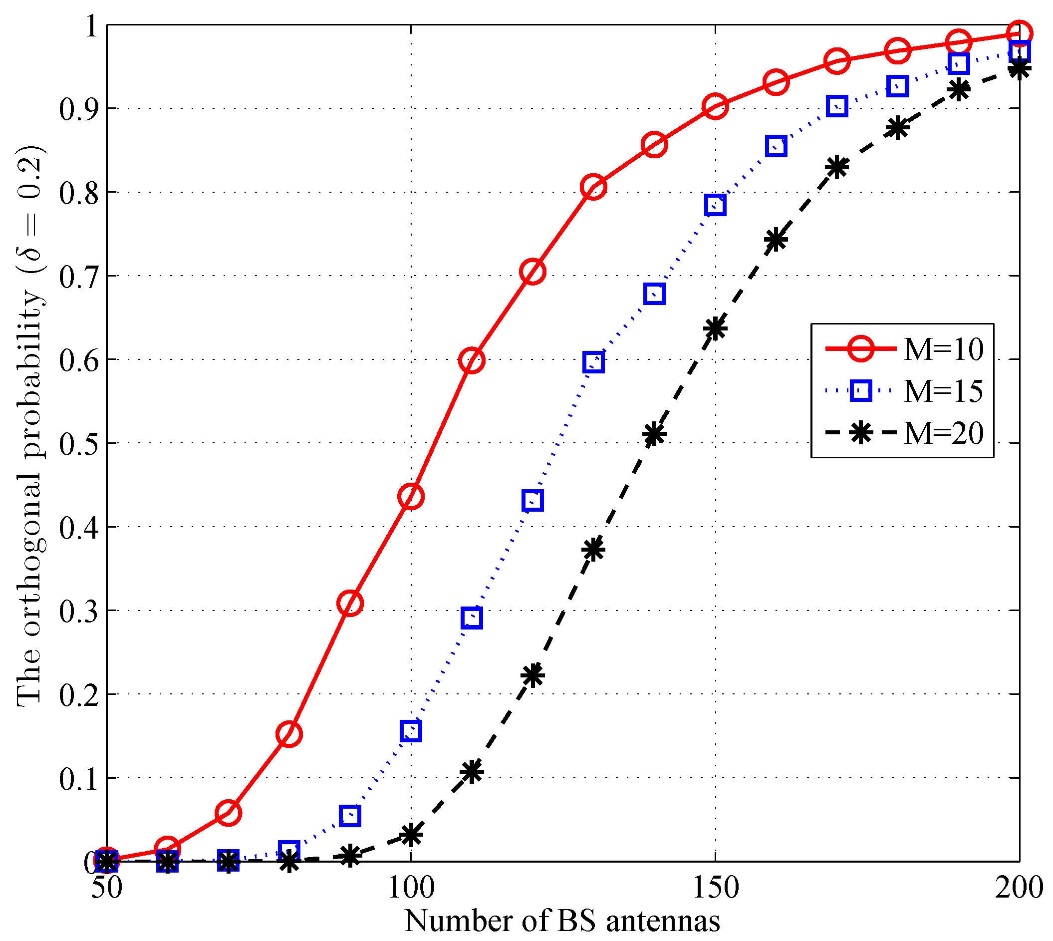
In this section, we first evaluate the asymptotical orthogonality of the channels between the BS and its served users, which reflects the computational efficiency of MRDS. Figure 1 shows the orthogonal probability ($\delta =0.2$) versus the number of BS antennas with $M=10$, 15, and 20. The orthogonal probability gets larger with the increase of the number of BS antennas or with the decrease of the user amounts.

In Figure 2 and Figure 3, the performance of the three proposed algorithms are compared to show the total power consumption and the computation time by 500 independent trials. In our experiments, we use the log-distance path loss model, in which the path loss at distance d is set as $\beta \left(d\right)\left[\mathrm{dB}\right]={\beta }_{fr}\left(d_0\right)+10nlog\left(\frac{d}{d_0}\right)$ [14], where n is the path loss exponent and ${\beta }_{fr}\left(d_0\right)$ is the free-space path loss at the reference distance $d_0$ and the carrier frequency of $f_c$. The simulation parameters are detailed in

Table 1. Simulation Parameters.

Parameter	Value	Parameter	Value
N	200	η	1
n	3.8	θ	0.8 W
$d_0$	100 m	${\sigma }_i^2$	−96 dBm
$P_{\mathrm{cir}}$	80 mW	$f_c$	2.5 GHz [10]

. Without loss of generality, All the users are assumed to be located 1200 m away from the BS, and all $\widetilde{{\gamma }_i}$s are the same and vary from 0 dB to 30 dB.

Figure 2 shows the average minimal total power consumption calculated by our methods versus the SNR constrains when $M=10$. The average minimal power consumption gets larger when the SNR requirement becomes more strictly. The difference of the average minimum total consumed power is minor between the RDS algorithm and the MRDS algorithm. The L0NM algorithm significantly outperforms the RDS algorithm, because it does not remove antennas randomly in each step as done by the RDS algorithm.

Figure 3 evaluates the average run time of our algorithms versus the SNR constrains when $M=10$. The codes are executed on a 64-bit desktop with 8 Gbyte RAM and Intel CORE i5 using YALMIP as the Matlab package. It can be seen that, either the MRDS algorithm or the L0NM algorithm provides noticeable improvement compared with the RDS algorithm in terms of the average run time.

5. Conclusions

We have studied in this paper how to jointly design the antenna selection and beamforming for the multicasting system with large-scale antenna arrays to minimize the total power consumption while guaranteeing the SNR requirement of each user. We proposed three decremental selection algorithms termed as RDS, MRDS, and L0MN. Performance results show that the L0NM algorithm can greatly outperform the random selection algorithm in terms of the total power consumption and the average run time.