2. Preliminaries
A graph is called outerplanar if it can be drawn on a plane such that all vertices lie on the outer face (i.e., the unbounded exterior region) without crossing of edges. Although there exist many embeddings (i.e., drawings on a plane) of an outerplanar graph, it is known that one embedding can be computed in linear time. Therefore, in this paper, we assume that each graph is given with its planar embedding. A path is called simple if it does not pass the same vertex multiple times. In this paper, a path always means a simple path that is not a cycle.
A
cut vertex of a connected graph is a vertex whose removal disconnects the graph. A graph is
biconnected if it is connected and does not have a cut vertex. A maximal biconnected subgraph is called a
biconnected component. A biconnected component is called a
block if it consists of at least three vertices; otherwise, it is an edge and called a
bridge. An edge in a block is called an
outer edge if it lies on the boundary of the outer face; otherwise, it is called an
inner edge. It is well-known that any block of an outerplanar graph has a unique Hamiltonian cycle, which consists of outer edges only [
20]. For the details of the terminology used in graphs and outerplanar graphs, refer to an appropriate textbook on graph theory (e.g., [
21]).
If we fix an arbitrary vertex of a graph G as the root r, we can define the parent-child relationship on biconnected components. For two vertices, u and v, u is called further than v if every simple path from u to r contains v. A biconnected component, C, is called a parent of a biconnected component if C and share a vertex v, where v is uniquely determined, and every path from any vertex in to the root contains v. In such a case, is called a child of C. A cut vertex v is also called a parent of C if v is contained in both C and its parent component ( both of a cut vertex and a biconnected component can be parents of the same component). Furthermore, the root, r, is a parent of C if r is contained in C.
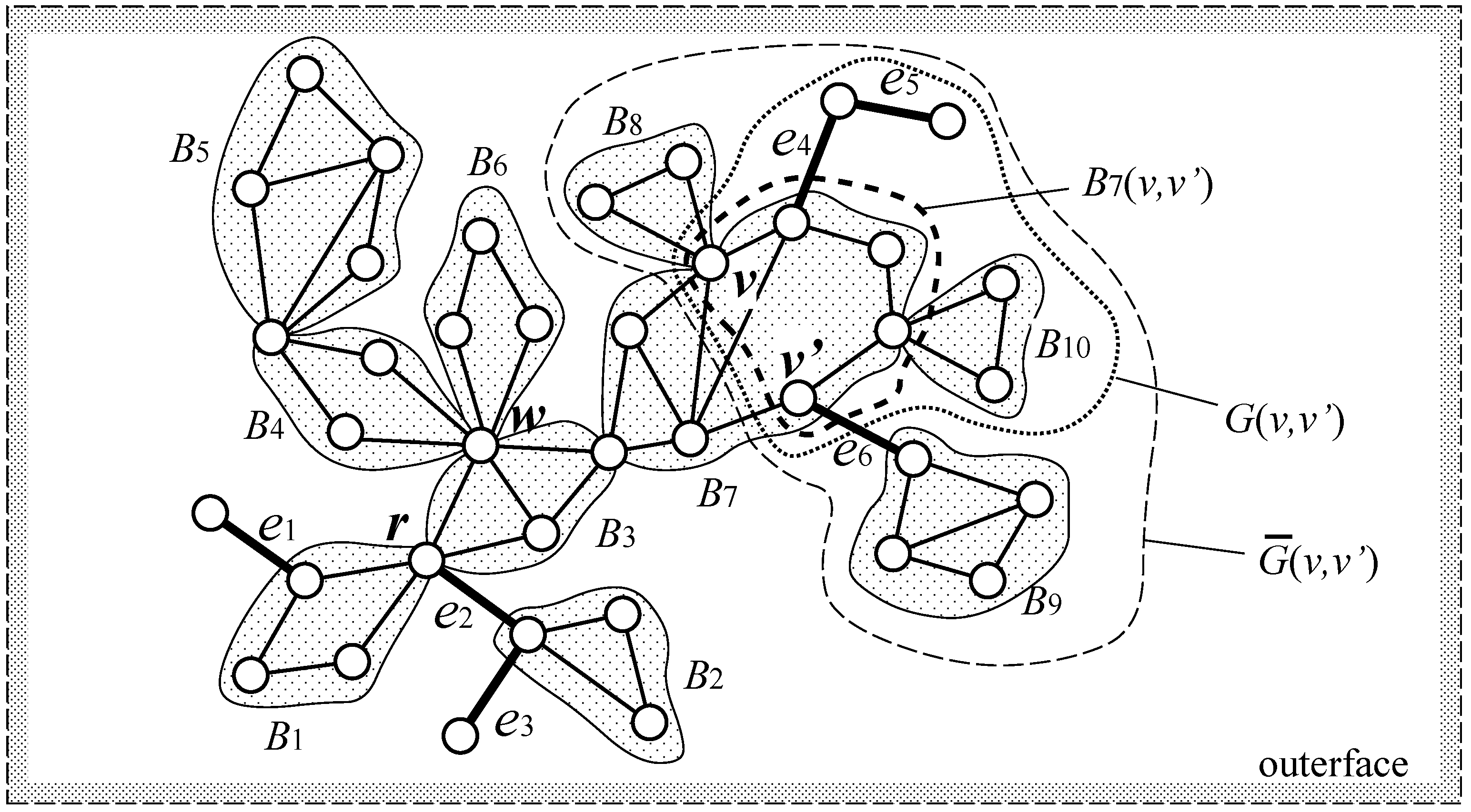
For each cut vertex v, denotes the subgraph of G induced by v and the vertices further than v. For a pair of a cut vertex v and a biconnected component, C, containing v, denotes the subgraph of G induced by vertices in C and its descendant components. For a biconnected component, B, with its parent cut vertex, w, a pair of vertices, v and , in B is called a cut pair if , and hold. For a cut pair in B, denotes the set of the vertices lying on the one of the two paths connecting v and in the Hamiltonian cycle that does not contain the parent cut vertex, except its endpoints. is the subgraph of B induced by and is called a half block. It is to be noted that contains both v and . Then, denotes the subgraph of G induced by and the vertices in the biconnected components, each of which is a descendant of some vertex in , and denotes the subgraph of G induced by the vertices in and descendant components of v and , where descendants are defined via the parent-child relationship.
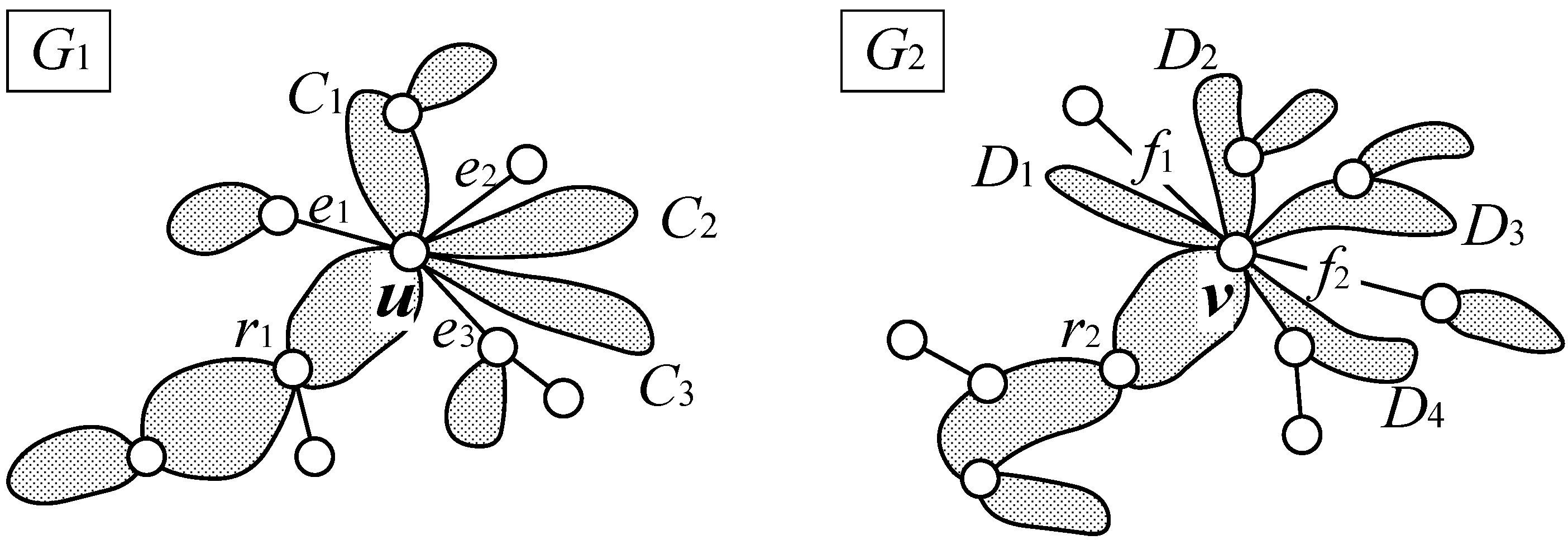
Example Figure 1 shows an example of an outerplanar graph
. Blocks and bridges are shown by gray regions and bold lines, respectively.
,
and
are the children of the root
r.
,
and
are the children of
, whereas
and
are the children of
w. Both
w and
are the parents of
and
.
consists of
,
and
, whereas
consists of
and
.
is a cut pair of
, and
is a region surrounded by a dashed bold curve.
consists of
,
,
,
,
,
and
, whereas
consists of
,
,
and
.
If a connected graph, , is isomorphic to a subgraph of and a subgraph of , we call a common subgraph of and . A common subgraph is called a maximum common connected edge subgraph of and if its size is the maximum among all common subgraphs (we use MCS to denote both the problem and the maximum common subgraph), where the size means the number of edges. In what follows, for the sake of simplicity, a maximum common subgraph (MCS) always means a maximum common connected edge subgraph. In this paper, we consider the following problem.
Figure 1.
Example of an outerplanar graph.
Figure 1.
Example of an outerplanar graph.
Maximum Common Subgraph of Outerplanar Graphs of Bounded Degree (OUTER-MCS)
Given two undirected connected outerplanar graphs, and , whose maximum vertex degree is bounded by a constant, D, find a maximum common subgraph of and .
Note that the degree bound is essential, because MCS is NP-hard for outerplanar graphs of unbounded degree, even if each biconnected component consists of at most three vertices [
9]. Although we do not consider labels on vertices or edges, our results can be extended to vertex-labeled and/or edge-labeled cases in which label information must be preserved in isomorphic mapping. In the following,
n denotes the maximum number of vertices of two input graphs ( it should be noted that the number of vertices and the number of edges are in the same order, since we only consider connected outerplanar graphs).
In this paper, we implicitly make extensive use of the following well-known fact [
13], along with outerplanarity of the input graphs.
Fact 1 Let and be biconnected outerplanar graphs. Let (resp. ) be the vertices of (resp. ) arranged in clockwise order in a planar embedding of (resp. ). If there is an isomorphic mapping from to a subgraph of , then appear in in either clockwise or counterclockwise order.
3. Algorithm for a Restricted Case
In this section, we consider the following restricted variant of OUTER-MCS, which is called SIMPLE-OUTER-MCS, and present a polynomial-time algorithm for it: (i) any two vertices in different biconnected components in a maximum common subgraph, , must not be mapped to vertices in the same biconnected component in (resp. ); (ii) each bridge in must be mapped to a bridge in (resp. ); (iii) the maximum degree need not be bounded.
It is to be noted from the definition of a common subgraph (regardless of the above restrictions) that no two vertices in different biconnected components in (resp. are mapped to vertices in the same biconnected component in any common subgraph, and no bridge in (resp. ) is mapped to an edge in a block in any common subgraph (otherwise there would exist a cycle containing the edge in a common subgraph, which would mean that the edge in (resp., ) is not a bridge).
SIMPLE-OUTER-MCS is intrinsically the same as the one studied by Schietgat
et al. [
11]. Although our algorithm is more complex and less efficient than their algorithm, we present it here, because the algorithm for a general (but bounded degree) case is rather involved and is based on our algorithm for SIMPLE-OUTER-MCS.
Here, we present a recursive algorithm to compute the size of MCS in SIMPLE-OUTER-MCS, which can be easily transformed into a dynamic programming algorithm to compute an MCS, as is true for many other dynamic programming algorithms. The following is the main procedure of the recursive algorithm.
Procedure
;
for all pairs of vertices do
Let be the root pair of ;
;
return .
The algorithm consists of a recursive computation of the following three scores:
- :
the size of an MCS between and , where is a pair of the roots or a pair of cut vertices, and must contain a vertex corresponding to both u and v.
- :
the size of an MCS between and , where is either a pair of blocks or a pair of bridges, u (resp. v) is the cut vertex belonging to both C (resp. D) and its parent, must contain a vertex corresponding to both u and v and must contain a biconnected component (which can be empty) corresponding to a subgraph of C and a subgraph D.
- :
the size of an MCS between and , where (resp. ) is a cut pair, and must contain a cut pair corresponding to both and . If there does not exist such (which must be connected), its score is .
In the following, we describe how to compute these scores.
Computation of
As in the dynamic programming algorithm for MCS for trees or almost trees [
9], we construct a bipartite graph and compute a maximum weight matching.
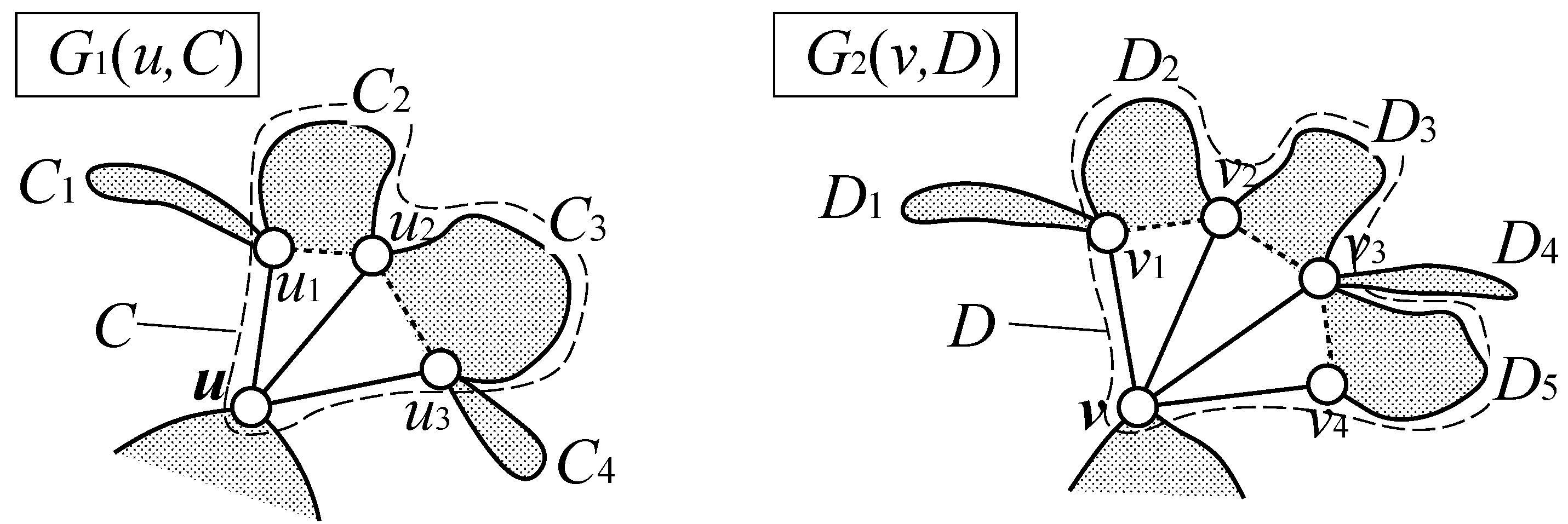
Let
and
be children of
u and
v respectively, where
’s and
’s are blocks and
’s and
’s are bridges (see
Figure 2). We construct an edge-weighted bipartite graph
by
Then, we let
be the weight of the maximum weight bipartite matching of
. It is to be noted that
(resp.,
) comes from the fact that
must be mapped to a bridge in
, but a bridge in
must not be mapped to an edge in any block (e.g.,
), because of the condition (ii) of SIMPLE-OUTER-MCS.
Figure 2.
Computation of .
Figure 2.
Computation of .
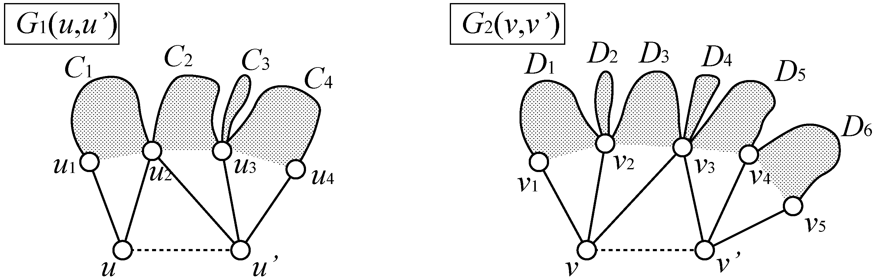
Computation of
Let
be the sequence of vertices in
, such that there exists an edge,
, for each
, where
are arranged in clockwise order.
is defined for
in the same way. It is to be noted that
is either a pair of blocks or a pair of bridges. A pair of subsequences
is called an
alignment if
and
or
hold ( the latter ordering is required for handling mirror images.), where
is allowed. We compute
by the following (see
Figure 3):
Procedure
;
for all alignments do;
if C is a block and then continue; /* blocks must be preserved */
;
for to g do ;
for to g do ;
;
return .
In the above procedure, the first inner
for loop takes care of blocks, such as
,
,
and
in
Figure 3, whereas the second inner
for loop takes care of half blocks, such as
,
,
,
and
in
Figure 3.
For example, consider an alignment,
, in
Figure 3, where all alignments are to be examined in the algorithm. Then, the score of this alignment is given by
.
comes via the computation of
, in which
is given by
,
,
, and thus, the maximum weight matching is given by
. In this case, an edge,
, is removed and then
is treated as a vertex on the path connecting
and
in the outer face. For another example, consider an alignment
in the same figure. Then, this alignment is ignored by the “
if ...
then ...” line of the procedure, because a bridge in
, which would correspond to
in
and
in
, must not be mapped to an edge in
C or
D. However, if both
and
are bridges, the resulting score would be
.
Figure 3.
Computation of .
Figure 3.
Computation of .
Since the above procedure examines all possible alignments, it may take exponential time. However, we can modify it into a dynamic programming procedure, as shown below, where we omit a subprocedure for handling mirror images, because it is trivial. In this procedure, and are processed from left to right. In the first for loop, stores the size of MCS between and plus one (corresponding to a common edge between and ). The double for loop computes an optimal alignment. stores the size of MCS between and up to and , respectively. is introduced to ensure the connectedness of a common subgraph. For example, if is a triangle, but is a rectangle. If C (and also D) is an edge, , but the procedure returns .
for all do
;
;
for to h do
for to k do
;
if then ;
if C is a block and then return 0 else return .
Computation of
Let be the sequence of vertices in , such that there exists an edge or for each , where are arranged in clockwise order. is defined for in the same way. For a pair, , if and hold, otherwise, . Similarly, for a pair, , if and hold, otherwise, . We compute by the following procedure, where it does not examine alignments with :
Procedure
if and then else ;
for all alignments do
if and hold for some t then continue;
if or holds then continue;
if and then else ;
for to g do;
for to g do ;
;
return .
This procedure returns if there is no connected common subgraph between and that contains corresponding to both and . It should be noted that the first line in the body of the main loop puts the constraint that all corresponding pairs, , in an alignment must be connected to either or , and the second line puts the constraint that must be connected to and must be connected to .
As an example, consider an alignment,
, in
Figure 4. Then, the score is given by
, where
is given via the computation of
.
Figure 4.
Computation of .
Figure 4.
Computation of .
For another example, the score is for each of alignments, , and , whereas the score of is 2, since , , , and . It is to be noted that vertices not appearing in an alignment can match in a later dynamic programming process; for example, can match with under an alignment of , although edges and are ignored.
As in the case of , can be modified into a dynamic programming version.
Then, we have the following theorem:
Theorem 1 SIMPLE-OUTER-MCS can be solved in polynomial time.
Proof. First we consider the correctness of the algorithm . The crucial points of the algorithm are that it examines all possible combinations of the neighbors via alignments examined in for each pair of cut vertices and via alignments examined in for each pair of cut pairs , where the connectedness in the latter case is taken care of by the use of and . It should be noted that non-neighbors of u cannot be neighbors of a node corresponding to u in MCS, and the ordering of neighbors must be preserved by Fact 1. Therefore, examination of all alignments covers all valid combinations of neighbors. Based on these facts, it is straightforward to see that correctly computes the size of MCS.
Next, we consider the time complexity. Since we examine possible root pairs, we focus on the case where the roots are fixed, where n is the maximum number of vertices in and .
Although is described as a recursive algorithm, the numbers of required scores of , and are , and , respectively. Therefore, by storing these values in some tables, we can transform into a dynamic programming algorithm.
Computation of
can be done in
time per call, because a maximum weight bipartite matching can be computed in
time [
22]. Using the dynamic programming version, the computation of each of
and
can be done in
time per call.
Therefore, the total time complexity is . ☐
Though it might be possible to substantially reduce the degree of polynomial by some simplification, as done in [
11], we do not go further, because our main purpose is to present a polynomial-time algorithm for the non-restricted (but bounded degree) case.
4. Algorithm for Outerplanar Graphs of Bounded Degree
In order to extend the algorithm in
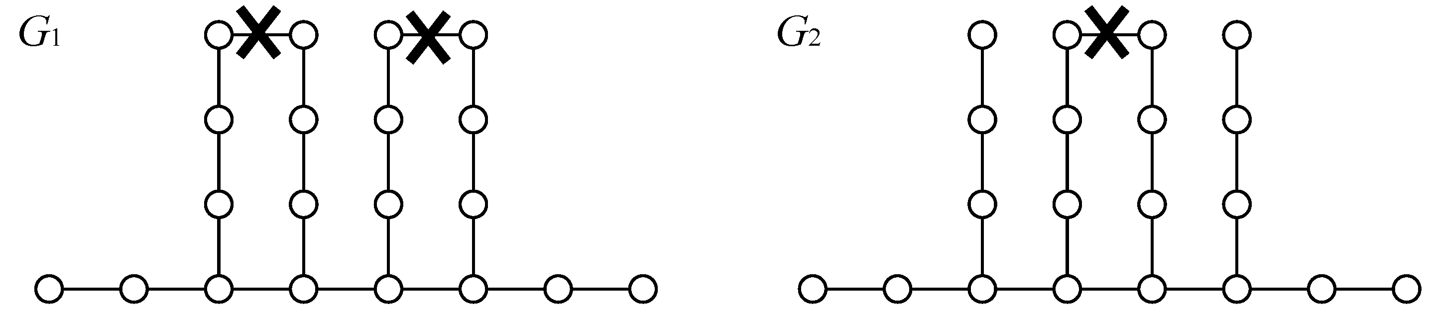
Section 3 for a general (but bounded degree) case, we need to consider the decomposition of biconnected components. For example, consider graphs
and
in
Figure 5. We can see that in order to obtain a maximum common subgraph, biconnected components in
and
should be decomposed, as shown in
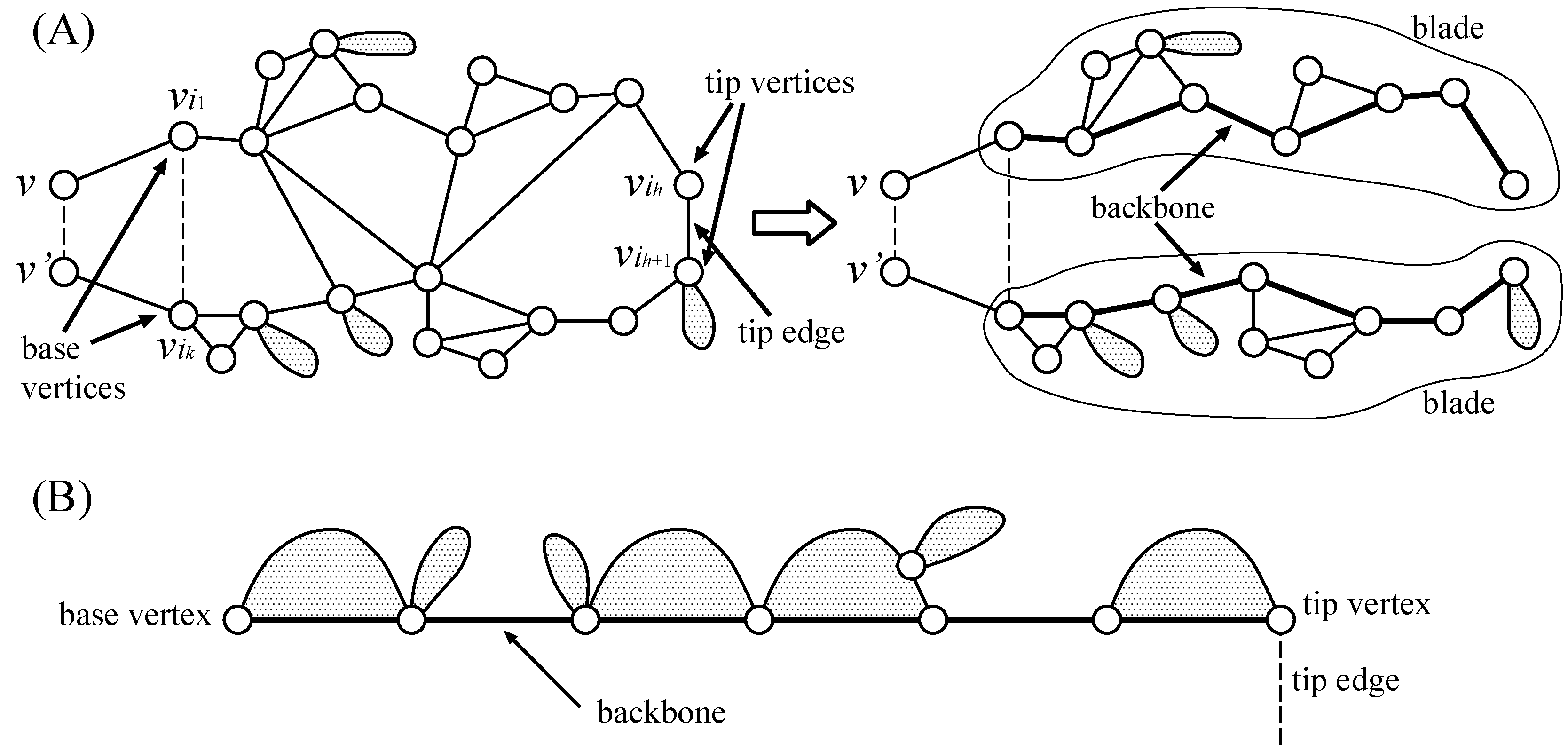
Figure 5, where there can be multiple ways of optimal decompositions in general. This is the crucial point, because considering all possible decompositions easily leads to exponential-time algorithms. In order to characterize decomposed components, we introduce the concept of a
blade, as shown below (see also
Figure 6).
Suppose that
are the vertices of a half block arranged in this order, and
and
are respectively connected to
v and
, where
v and
can be the same vertex. If we cut one edge,
for
, we obtain two half blocks, one induced by
and the other induced by
. However, only one half block is obtained in the case of
or
, and no half block is obtained in the case of
(see
Figure 7). Each of these half blocks is a chain of biconnected components called a
blade body, and a subgraph consisting of a blade body and its descendants is called a
blade. Vertices
and
, an edge
and vertices
are called
base vertices, a
tip edge and
tip vertices, respectively. The sequence of edges in the shortest path from
to
(resp. from
to
) is called the
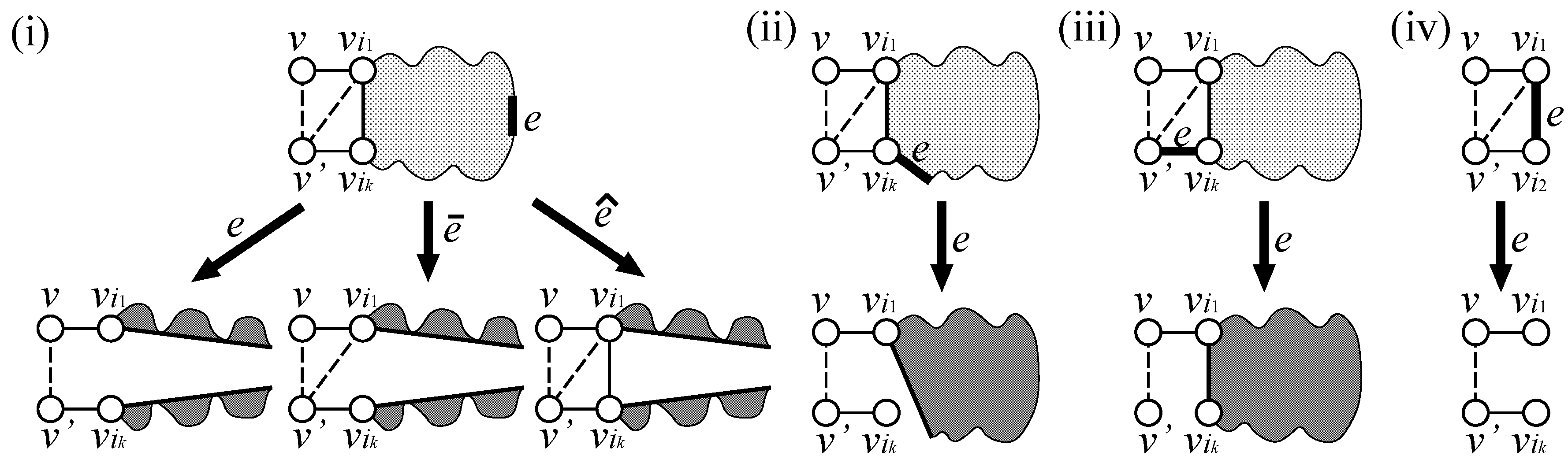
backbone of a blade. As a result, the edges between two blades are deleted (it does not cause a problem, because all possible configurations are examined, as discussed later). In addition, there exists three subcases, depending on the existence of edges
and
(cases with
can be handled in an analogous way). We need not consider the case where
is deleted, but
remains, because deletion of
can be handled in the computation of
):
both and are deleted
is deleted, but remains
both and remain
where these three cases are respectively denoted by “deletion of
e”, “deletion of
” and “deletion of
” (see
Figure 7). It is to be noted that, in any case, we cannot have multiple tip edges simultaneously for the same pair,
, because disconnected component(s) would appear if multiple tip edges exist.
Figure 5.
Example of a difficult case.
Figure 5.
Example of a difficult case.
Figure 6.
(A) Construction of blades where subgraphs, excluding gray regions (descendant components), are blade bodies; and (B) schematic illustration of a blade.
Figure 6.
(A) Construction of blades where subgraphs, excluding gray regions (descendant components), are blade bodies; and (B) schematic illustration of a blade.
Figure 7.
Types and subcases of blades, where two other subcases for (ii) and another subcase (i.e., remains) for (iii) and (iv) are omitted.
Figure 7.
Types and subcases of blades, where two other subcases for (ii) and another subcase (i.e., remains) for (iii) and (iv) are omitted.
In addition, we allow
(resp.
) to be a tip edge. In this case, after removing this tip edge, the resulting half block induced by
(resp.
) is a blade body, where
(resp.
) becomes the base vertex. For example, the rightmost blade in
Figure 8 is created by removing a tip edge
and
becomes the base vertex.
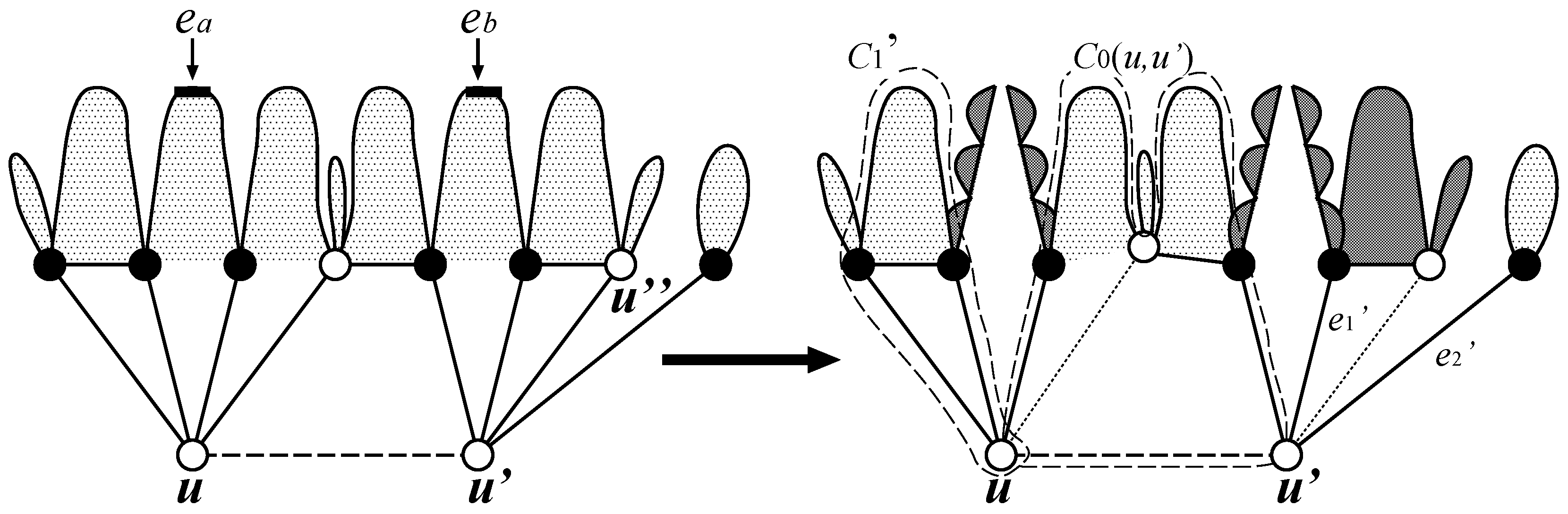
Figure 8.
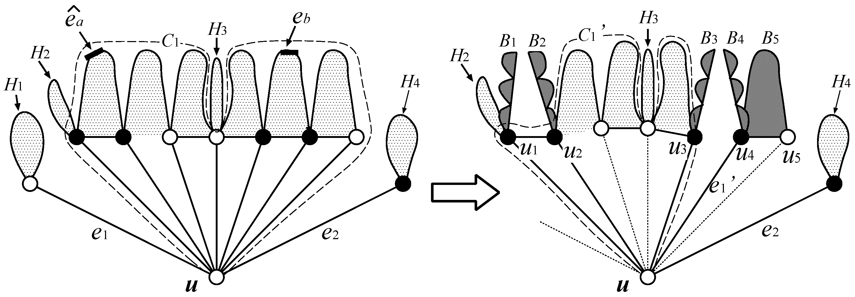
Example of configuration and its resulting subgraph of . Black circles, dark gray regions and thin dotted lines denote selected vertices, blades and removed edges, respectively. Block and edges are the children of u in , where block is a child of , blocks are children of and block is a child of . Edges, , are tip edges, where is also regarded as a tip edge. Then, edge is deleted along with block , whereas edge remains as it is. Block is divided into block , blades and edge , where blocks, , and blades, , are children of and blades, , are children of . In the resulting subgraph, block, , and edges, , are the children of u.
Figure 8.
Example of configuration and its resulting subgraph of . Black circles, dark gray regions and thin dotted lines denote selected vertices, blades and removed edges, respectively. Block and edges are the children of u in , where block is a child of , blocks are children of and block is a child of . Edges, , are tip edges, where is also regarded as a tip edge. Then, edge is deleted along with block , whereas edge remains as it is. Block is divided into block , blades and edge , where blocks, , and blades, , are children of and blades, , are children of . In the resulting subgraph, block, , and edges, , are the children of u.
Since a blade can be specified by a pair of base and tip vertices and an orientation (clockwise or counterclockwise), there exist blades in and . Of course, we need to consider the possibility that during the execution of the algorithm, other subgraphs may appear from which new blades are created. However, we will show later that blades appearing in the algorithm are restricted to be those in and .
4.1. Description of Algorithm
In this subsection, we describe the algorithm as a recursive procedure, which can be transformed into a dynamic programming one, as stated in
Section 3.
The main procedure,
is the same as that mentioned in
Section 3, and we recursively compute three kinds of scores:
,
and
, where cut vertices, cut pairs, blocks and bridges do not necessarily mean those in the original graphs, but may mean those in subgraphs generated by the algorithm.
Computation of
Let
and
be children of
u, where
’s and
’s are blocks and bridges, respectively. Let
be the neighboring vertices of
u that are contained in the children of
u. We define a
configuration as a tuple of the following (see
Figure 8).
- for :
means that is selected as a neighbor of u in a common subgraph, otherwise . is called a selected vertex if .
- :
is an edge in , where B is the block containing , and u. This edge is defined only for a consecutive selected vertex pair, and , in the same block (i.e., does not contain any other selected vertex). e is used as a tip edge, where e can be empty, which means that we do not cut any edge in . It is to be noted that, at most, one edge in can be a tip edge, and thus, each is divided into, at most, two blade bodies; further decomposition will be done in later steps. We also consider and for whenever available.
Each configuration defines a subgraph of
as follows:
() remains if . Otherwise, is removed along with its descendants.
If no vertex in is selected, it is removed along with its descendants. Otherwise, is divided into blocks, blade bodies (according to ’s and ’s) and bridges, where edges, with , are removed.
Let
and
be the resulting blocks and bridges containing
u, which are new `children’ of
u, for a configuration,
. Configurations are defined for
in an analogous way. Let
and
be the resulting new children of
v for a configuration
of
. As stated in
Section 3, we construct a bipartite graph
by
and we compute the weight of the maximum weight matching for each configuration pair
( although a bridge cannot be mapped on a block here, a bridge can be mapped to an edge in a block of an input graph by converting the block into smaller blocks and bridges using tip edge(s)). The following is a procedure for computing
:
Procedure
;
for all configurations for do
for all configurations for do
weight of the maximum weight matching of ;
if then ;
return .
Computation of
This score can be computed, as stated in
Section 3, although we should take blades into account. In this case, we can directly examine all possible alignments, because the number of neighbors of
u or
v is bounded by a constant, and we need to examine a constant number of alignments.
Computation of
As in
, we examine all possible configurations by specifying selected vertices and tip edges (see
Figure 9). Each configuration defines a subgraph of
(resp.
). This subgraph contains three kinds of biconnected components:
- (i)
components connecting only to u (resp. v)
- (ii)
components connecting only to (resp. ) and
- (iii)
component connecting to both u and (resp. v and ), where this type (iii) component is uniquely determined.
Figure 9.
Example of configuration and its resulting subgraph for . Black circles, dark gray regions and thin dotted lines denote selected vertices, blade, and removed edges, respectively. Edges, , are tip edges, where is also regarded as a tip edge. In the resulting subgraph, is a type (i) component, and are type (ii) components and is a type (iii) component.
For each of type (i) and type (ii) components, we construct a bipartite graph, as in , although blades might appear in the recursive process. Let the resulting bipartite graphs be and , respectively. Let and be type (iii) components (i.e., half blocks) for and , respectively. For this pair of components, we compute a maximum common subgraph, as in . The following is a pseudocode of :
Procedure
;
for all configurations for do
for all configurations for do
score of the maximum common subgraph between and ;
weight of the maximum weight matching of ;
weight of the maximum weight matching of ;
if then ;
return .
4.2. Analysis
As mentioned before, each blade is specified by base and tip vertices in or and an orientation. Each half block is also specified by two vertices in a block in or . We show that this property is maintained throughout the execution of the algorithm and bound to the number of half blocks and blades, as below.
Lemma 1 The number of different half blocks and blades appearing in is .
Proof. We prove it by mathematical induction on the number of steps in the execution of the algorithm. At the beginning of the algorithm, this property is trivially maintained, because we only have
and
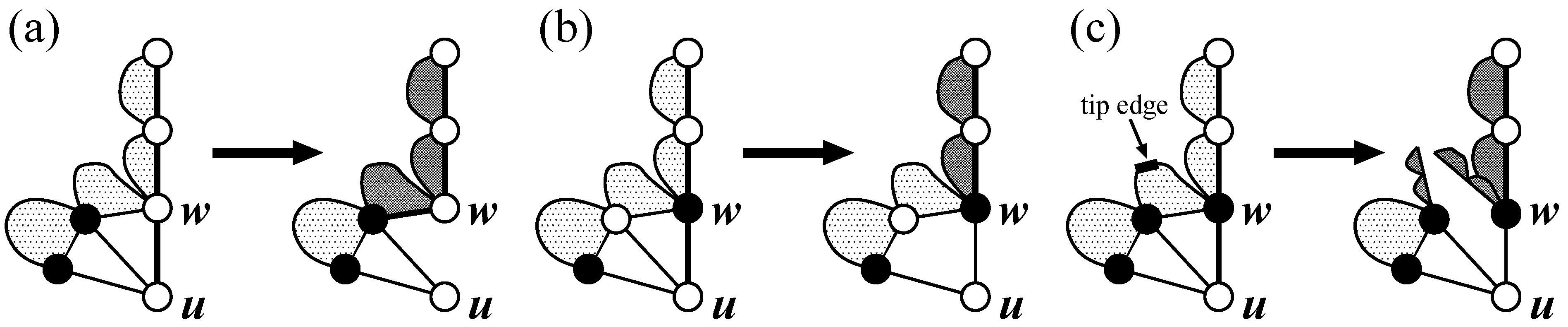
. A new half block (along with its descendants) or a new blade is created only when graphs are modified according to a configuration or alignment. In the alignment case, it is straightforward to see that new half blocks are half blocks of the current block or current half block. It can also be seen that whenever a blade is newly created, it is a half block (along with descendants) of the current block or current half block. The crucial cases lie when an existing blade is modified according to a configuration. Let
u and
be the base vertex and a backbone edge in a blade
, respectively. Let
be the block in
(resp.
) from which
was created. Then, we need to consider the following three cases (
Figure 10) ( new blades may also be created by a tip edge in a half block specified by a pair of selected vertices):
- (a)
w is not selected.
The base vertex of a new blade is the selected vertex nearest to w in the first block (i.e., block containing u) of . Since the original blade body was a half block of a block , the resulting blade body is also a half block of .
- (b)
w is selected, and there is no tip edge between w and its nearest selected vertex.
The resulting blade body begins from w (in the next step), which is a half block of .
- (c)
w is selected, and there is a tip edge between w and its nearest selected vertex.
The resulting blade body begins from w, which is a half block of . Furthermore, two (or less) new blade bodies are created, both of which are half blocks of .
Therefore, we can see that every half block or blade appearing in the algorithm is specified by two vertices in a block of
or
, from which the lemma follows. ☐
Figure 10.
Three cases considered in the proof of Lemma 1. Bold lines and dark gray regions denote backbone edges and new blade bodies, respectively.
Figure 10.
Three cases considered in the proof of Lemma 1. Bold lines and dark gray regions denote backbone edges and new blade bodies, respectively.
Finally, we obtain the following theorem.
Theorem 2 A maximum common connected edge subgraph of two outerplanar graphs of bounded degree can be computed in polynomial-time.
Proof. It is straightforward to check the correctness of the algorithm, because it implicitly examines all possible common subgraphs via alignment, decomposition by configurations and bipartite matching, where Fact 1 enables us to use alignment and dynamic programming. Therefore, we focus on the time complexity.
Since the number of half blocks and blades is and the maximum degree is bounded, the number of different ’s and ’s (resp. ’s and ’s) appearing in the algorithm, some of which can be obtained from subgraphs of (resp. ), is , where an additional factor comes from the fact that new blocks and bridges may be created per blade. Therefore, we can transform the recursive algorithm into a dynamic programming algorithm using size tables.
For each subgraph appearing in
or
as an argument, the number of configurations is
, because there exists at most
neighboring vertices (excluding those nearer to the root) of
u and
(resp.
v and
) for a constant,
D, (
) and a tip edge lies between a path connecting two neighboring vertices. For some block pair, we need to examine all possible alignments. Since the maximum degree is bounded by constant,
D, we need to examine a constant number of alignments, and thus, this calculation can be done in constant time. By the same reason, a maximum matching can be computed in constant time. All other miscellaneous operations, which include modification of edges and summation of scores, can be performed in
time per pair of configurations, pair of biconnected components and pair of half blocks. Since we need to examine
pairs of the roots, the total computation time is:
for a constant,
D (a constant factor depending only on
D is ignored here, because we assume that
D is a constant). ☐

